www.geosci-model-dev.net/9/2239/2016/ doi:10.5194/gmd-9-2239-2016
© Author(s) 2016. CC Attribution 3.0 License.
Improving the WRF model’s (version 3.6.1) simulation over sea ice
surface through coupling with a complex thermodynamic sea ice
model (HIGHTSI)
Yao Yao1,2, Jianbin Huang1, Yong Luo1, and Zongci Zhao1
1Ministry of Education Key Laboratory for Earth System Modeling, Center for Earth System Science, Tsinghua University,
Beijing, China
2International Laboratory on Climate and Environment Change and Key Laboratory of Meteorological Disaster,
Nanjing University of Information Science and Technology, Nanjing, China Correspondence to:Jianbin Huang ([email protected])
Received: 8 September 2015 – Published in Geosci. Model Dev. Discuss.: 3 December 2015 Revised: 9 May 2016 – Accepted: 23 May 2016 – Published: 28 June 2016
Abstract. Sea ice plays an important role in the air–ice– ocean interaction, but it is often represented simply in many regional atmospheric models. The Noah sea ice scheme, which is the only option in the current Weather Research and Forecasting (WRF) model (version 3.6.1), has a prob-lem of energy imbalance due to its simplification in snow processes and lack of ablation and accretion processes in ice. Validated against the Surface Heat Budget of the Arctic Ocean (SHEBA) in situ observations, Noah underestimates the sea ice temperature which can reach −10◦C in winter. Sensitivity tests show that this bias is mainly attributed to the simulation within the ice when a time-dependent ice thick-ness is specified. Compared with the Noah sea ice model, the high-resolution thermodynamic snow and ice model (HIGH-TSI) uses more realistic thermodynamics for snow and ice. Most importantly, HIGHTSI includes the ablation and accre-tion processes of sea ice and uses an interpolaaccre-tion method which can ensure the heat conservation during its integra-tion. These allow the HIGHTSI to better resolve the energy balance in the sea ice, and the bias in sea ice temperature is reduced considerably. When HIGHTSI is coupled with the WRF model, the simulation of sea ice temperature by the original Polar WRF is greatly improved. Considering the bias with reference to SHEBA observations, WRF-HIGHTSI im-proves the simulation of surface temperature, 2 m air temper-ature and surface upward long-wave radiation flux in winter by 6, 5◦C and 20 W m−2, respectively. A discussion on the impact of specifying sea ice thickness in the WRF model is presented. Consistent with previous research, prescribing the
sea ice thickness with observational information results in the best simulation among the available methods. If no observa-tional information is available, we present a new method in which the sea ice thickness is initialized from empirical esti-mation and its further change is predicted by a complex ther-modynamic sea ice model. The ice thickness simulated by this method depends much on the quality of the initial guess of the ice thickness and the role of the ice dynamic processes.
1 Introduction
Although climate models have become more sophisti-cated, climate simulation over the polar region remains a formidable challenge (Notz, 2012; Bourassa et al., 2013). The surface radiance budget, which exhibits marked seasonal differences between summer and winter and plays an impor-tant role in the polar climate system, has been erroneously represented in climate models for a long time (Sorteberg et al., 2007; Tjernström et al., 2008; Barton et al., 2014). From a perspective from the top of the atmosphere to the surface, researchers have attributed the bias of the surface ra-diation budget to the poor ability of models to properly rep-resent both the cloud radiation effect and the stable bound-ary layer (Wyser et al., 2007; Vihma and Pirazzini, 2005). The Arctic cloud, particularly the mixed-phase low cloud, is misrepresented in current state-of-the-art climate models (Pithan et al., 2013; English et al., 2015). Simulating the stable boundary layer is limited not only by the relatively coarse resolution (Steeneveld et al., 2006), but also by the lack of realistic representations of small-scale physical pro-cesses, such as turbulent mixing and snow-surface coupling (Sterk et al., 2013). As a result, considerable effort has been devoted to evaluating and improving the microphysics and boundary layer parameterizations (e.g., Wang and Liu, 2014; Andreas et al., 2010).
Besides the cloud and boundary layer processes, sea ice, which distinguishes the polar climate system from other parts of the earth system, is also an essential factor for a realistic simulation of polar climate. When the ocean is covered by sea ice, the exchange of heat between air and sea and the pen-etration of solar radiation differ significantly from over open water. Acting as a medium between air and sea, sea ice plays an important role in the surface energy balance over the po-lar region (Jin et al., 1994). Thus, a realistic simulation of the polar climate requires sea ice to be appropriately considered in the RCMs. Coupled RCMs, including interactive ocean and sea ice models, have shown benefits from a better repre-sentation of the air–ice–ocean interaction (Dorn et al., 2009). However, the relatively large resources that are required to construct the coupled modeling system and the insufficient simulation of feedbacks between the model components have limited the use of coupled RCMs (Dorn et al., 2012). To meet the urgent needs of research and applications from different fields, atmospheric-only RCMs are still widely used in simu-lations of the polar climate. In these models, sea surface tem-perature and sea ice concentration have to be specified, and the surface properties of sea ice are determined by thermody-namic sea ice models. However, the sea ice models incorpo-rated in current RCMs often lack detailed treatments of ther-modynamic processes. As the lower boundary condition for the atmospheric model, the simplified thermodynamic sea ice model could exert biased forcing to the atmosphere (Valko-nen et al., 2014). To overcome this problem, efforts have been made in order to better represent the sea ice in RCMs. For example, studies have shown that properly specifying the sea ice thickness and snow on ice have a considerable impact
on the simulation of surface temperature (Rinke et al., 2006; Hines et al., 2015).
Among the atmospheric-only RCMs, the Weather Re-search and Forecasting (WRF) model, along with its polar-optimized version (Polar WRF), has been widely used in po-lar climate simulations. Previous evaluations have shown that the WRF model can reasonably simulate climatological fea-tures of the Arctic atmosphere (Cassano et al., 2011). Addi-tionally, physical credibility has been found in simulating ex-treme precipitation over CORDEX Arctic from a long-term climate simulation based on the WRF model (Glisan and Gutowski, 2014a, b). Moreover, the modifications included in the Polar WRF model have been validated against vari-ous observations in Greenland (Hines and Bromwich, 2008), the Arctic Ocean (Bromwich et al., 2009), Arctic land (Hines et al., 2011) and the Antarctic (Bromwich et al., 2013). In ad-dition to the above validations, the open access of the WRF model means that it has been widely applied in polar research by a large number of users.
Despite the previous sea ice enhancements that have al-ready been included in the Polar WRF model (Bromwich et al., 2009; Hines et al., 2015), a simplified thermodynamic sea ice model (Noah scheme) is still the only option to de-scribe sea ice status. This means simplifications and lack of important thermodynamic processes exist in the current WRF and Polar WRF (version 3.6.1). These shortages in the model can lead to a problem of energy imbalance in snow and ice, which is an important issue in regional climate simula-tion. For example, the Noah sea ice scheme does not include the ice ablation and accretion processes and it prevents the snow depth from falling below 0.01 m. These issues can lead to a problem of energy imbalance in snow and ice (Valkonen et al., 2014), and a more advanced scheme for sea ice and snow should be used to improve the simulation. Currently, there are few evaluations of the performance of a simplified sea ice model when it is used as part of a RCM during long-term climate simulations. How well does Noah sea ice within the WRF model represent the long-term evolution of sea ice status? Due to the large number of WRF users, a further de-velopment of the WRF model would benefit a wide range of research. To improve the simulation over the polar region by the WRF model, it is worth testing the possible added value from coupling a complex thermodynamic sea ice model. Can the simulation over the sea ice surface benefit from a more re-alistic simulation of sea ice thermodynamics? As mentioned above, additional information on sea ice thickness needs to be specified when the atmospheric-only RCM is used in polar climate simulations. How is the sea ice thickness prescribed if a complex sea ice model is coupled to the RCM? This study is conducted based on the above questions.
model, and the coupled simulations based on Noah and the HIGHTSI sea ice model are compared in Sect. 4. The evalu-ation is primarily focused on the simulevalu-ation over the sea ice surface to determine whether coupling a complex thermody-namic sea ice model would be beneficial for regional climate simulations. In Sect. 5, we present a discussion on how to prescribe the sea thickness in an atmospheric-only regional climate simulation.
2 Models and data 2.1 WRF
The WRF model is a state-of-the-art mesoscale numerical model designed for both research and operations. It is primar-ily maintained by the National Centers for Atmospheric Re-search (NCAR) and developed by collaborative efforts from the community. The WRF model has been widely used in climate simulations, and its applications in the polar region have also provided useful information (Liu et al., 2014). Po-lar WRF is a poPo-lar-optimized version released after the stan-dard WRF model. Modifications such as fractional sea ice and optimized surface energy balance over land ice and sea ice have enabled the model to better simulate the polar cli-mate (Hines and Bromwich, 2008). Moreover, some of these changes have already been added to recent versions of stan-dard WRF releases.
In both WRF and Polar WRF, a simplified thermodynamic sea ice model that is included in the Noah land surface model is used to determine the sea-ice-related properties, such as sea ice temperature and turbulent fluxes. The Noah sea ice module incorporated in WRF contains four-layer ice together with a single-layer snowpack model. The ice growing and ablation processes are not included in Noah, and thus, the sea ice thickness must be specified. The default value for sea ice thickness is 3 m everywhere in the WRF model, and this value can be prescribed from other sources in the same way as sea ice concentration such that the spatial and tempo-ral variations of sea ice thickness can be taken into account (Hines et al., 2015). The sea ice surface is assumed to always be covered by snow in Noah, and a lower bound (default is 0.01 m) for snow depth has to be prescribed. Under this as-sumption, the surface energy balance would always be evalu-ated over a snow surface. The solar radiation is allowed to be absorbed only by the snow layer; thus, no solar penetration into the ice is considered.
There are three schemes for treating the sea ice albedo in the Noah sea ice module. One is a fixed value for the albedo; thus, seasonal variation and spatial distribution would not be taken into consideration. Another scheme uses the observed albedo through additional input data. The other scheme, which estimates the albedo as a function of surface temper-ature, is used in this study. Previous studies have shown that this empirical estimation of sea ice albedo could provide a
re-sult close to that obtained from observations in the Arctic during the summer melt season (Bromwich et al., 2009).
2.2 HIGHTSI
HIGHTSI was initially designed for seasonal ice simulation (Launiainen and Cheng, 1998; Vihma et al., 2002; Cheng et al., 2006), and it is also capable of being applied over perennial sea ice (Cheng et al., 2008b). Previous evaluations have shown that HIGHTSI can simulate the seasonal evolu-tion of Arctic sea ice temperature and thickness well (Cheng et al., 2008b, 2013). Further studies have extended the use of HIGHTSI in investigating various processes. By combin-ing the modelcombin-ing with HIGHTSI and remote senscombin-ing data, an analysis that can better reveal the sea ice thickness and con-centration information has been conducted (Karvonen et al., 2012). Moreover, HIGHTSI has also been used in lake ice studies (Yang et al., 2012), and its benefits from a detailed treatment of snow and ice thermodynamics were confirmed when compared with a simple lake model (Semmler et al., 2012).
HIGHTSI contains multi-layer (up to 100) snow and ice such that the heat conduction in snow and ice can be rep-resented in greater detail, and the convergence of the non-linear temperature solver can be better resolved (Dupont et al., 2015). Following the recommendations by Cheng et al. (2008a), all the simulations in the study use 10 layers for snow and 20 layers for ice. The melt is calculated for each layer of snow and ice where the temperature would rise above the freezing point. After being reflected by the surface of sea ice and absorbed in the snow layer, the solar radiation is then allowed to penetrate into the ice layers in HIGHTSI. Dur-ing the ice melt season, the penetration of solar radiation into the ice layer can warm the sea ice, thus causing ice abla-tion. The surface of sea ice in HIGHTSI is treated differently when it is covered by snow such that a more realistic sea-sonal feature of the sea ice surface can be represented in the model. The surface conductive heat flux would be calculated for the interface between the surface and the uppermost snow layer for snow surface, and between the surface and the up-permost ice layer for the bare ice surface. Benefiting from the detailed representation of heat conduction and solar pen-etration in the sea ice, HIGHTSI is able to predict the change in sea ice thickness caused by thermodynamic ablation and accretion processes. HIGHTSI utilizes the sigma-coordinate for both snow and ice layers. When the snow and ice thick-ness changes, an interpolation step which can ensure the con-servation of heat is performed. More detailed technical infor-mation of HIGHTSI can be found in Launiainen and Cheng (1998).
and ice thickness. Note that the CCSM scheme used in this study does not including the input of the depth of melt ponds; thus it only considers the effect of melt ponds implicitly through its relationship with surface temperature.
Some modifications have been made to the snow processes in the original HIGHTSI model such that it can share some common physical assumptions with the snow over land and ice sheets in the WRF modeling system. The snow sublima-tion over sea ice is calculated using the same Penman equa-tion used over land and ice sheets. The snow conducequa-tion as a function of snow density and the snow compaction effect as a function of temperature and time are also in accord with the empirical methods originally used by the Noah land surface module in WRF.
Compared with the Noah sea ice, HIGHTSI is more com-plex and shows advantages on several aspects. First, HIGH-TSI has more vertical layers for both snow and ice than Noah, which means the vertical profile of temperature within snow and ice can be represented in greater detail in HIGHTSI than in Noah. Moreover, the surface and basal accretion and ab-lation processes of sea ice are included in HIGHTSI. Un-like Noah in which the sea ice thickness has to be specified, HIGHTSI can predict the change in sea ice thickness itself. A self-adapted ice thickness is crucial for the conservation of energy in sea ice. When the ice thickness is kept constant or specified inappropriately, a misrepresentation of energy bal-ance happens. Another problem that has been found in Noah is the treatment of sea ice surface. The Noah model assumes the surface of sea ice to be always covered by snow, and a lower bound of 0.01 m is set to prevent the snow depth from becoming too thin. As what has been found in Valkonen et al. (2014), this assumption could lead to a problem of energy imbalance in the simulation of sea ice by Noah. HIGHTSI, on the other hand, includes different treatments for snow and bare ice surface. When the snow is thin or melted, the so-lar radiance, which has penetrated into the ice, could further heat and melt the ice. Unlike Noah which only considers the solar radiation absorbed by the snow layer, HIGHTSI takes the penetration of solar radiation in both snow and ice layers into consideration.
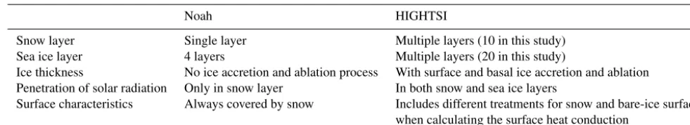
A summary of the major differences between Noah and HIGHTSI can be found in Table 1.
We added the HIGHTSI sea ice model as an option in the WRF modeling system such that it could be easily switched to use the Noah sea ice (hereafter WRF-Noah) or the HIGH-TSI (hereafter WRF-HIGHHIGH-TSI) sea ice through specifying a flag in the namelist file. Both Noah and HIGHTSI utilize the same time step with the WRF model, and they are cou-pled with WRF at every step. When using the HIGHTSI op-tion, the WRF model would provide precipitaop-tion, surface downward long-wave and shortwave radiation, and air tem-perature, wind speed and height of the lowest model level to drive the HIGHTSI model. HIGHTSI provides the updated surface temperature, albedo, emissivity, upward water vapor
flux and sensible and latent heat flux to WRF, which then influence the atmospheric processes in the boundary layer. 2.3 Data
The Surface Heat Budget of the Arctic Ocean (SHEBA) ex-periment during 1997–1998 made comprehensive observa-tions of the atmosphere, ocean and sea ice available (Ut-tal et al., 2002). The surface temperature, ice mass bal-ance and ice temperature profiles are used to validate the sea ice simulation in this study. The atmospheric observa-tions and the surface radiation observaobserva-tions are not only used in the model evaluations, but are also used as forc-ing data to drive the stand-alone versions of Noah sea ice and HIGHTSI. To validate the simulation over the entire model domain, satellite observations are also used. They are the skin surface temperature data from the Extended Ad-vanced Very High Resolution Radiometer (AVHRR) Polar Pathfinder (APP-x) product (Key et al., 1997) and the sur-face shortwave and long-wave radiation data from the Eu-ropean Organisation for the Exploitation of Meteorological Satellites (EUMETSAT) Climate Monitoring Satellite Ap-plication Facility (CM SAF) CLoud, Albedo and RAdiation dataset from AVHRR data (CLARA-A1) (Karlsson et al., 2013). Both APP-x and CLARA-A1 have similar spatial res-olutions (25 km and 0.25◦, respectively) to that used in our climate simulations. Validations with in situ observations have shown that both APP-x and CLARA-A1 have accept-able accuracies, and these products have already been used in model evaluations and climate change studies over the Arctic (Wang and Key, 2003; Svensson and Karlsson, 2011; Karls-son and SvensKarls-son, 2013; Koenigk et al., 2014; Riihelä et al., 2013).
3 Offline simulation of sea ice
Table 1.Summary of the major differences between Noah and HIGHTSI
Noah HIGHTSI
Snow layer Single layer Multiple layers (10 in this study)
Sea ice layer 4 layers Multiple layers (20 in this study)
Ice thickness No ice accretion and ablation process With surface and basal ice accretion and ablation Penetration of solar radiation Only in snow layer In both snow and sea ice layers
Surface characteristics Always covered by snow Includes different treatments for snow and bare-ice surface when calculating the surface heat conduction
Figure 1.Topography of the simulation domain. SHEBA site loca-tions are marked by the black curve.
can be found in Huwald et al. (2005). The simulations start on 31 October 1997 and end on 22 September 1998 accord-ing to the temporal coverage of SHEBA data at the Pittsburgh site. The locations of the site are shown in Fig. 1. The sea ice thickness is updated at every simulation step by the SHEBA observations for the Noah sea ice module because it is not able to predict the change in sea ice thickness. Benefiting from the more detailed description of thermodynamic pro-cesses of the sea ice in HIGHTSI, the sea ice thickness is predicted by the model itself for the HIGHTSI offline run. As mentioned above, snow is assumed to always exist over the sea ice in Noah, and thus, a lower bound for snow depth needs to be specified. In this study, the minimum snow depth in Noah is set to 0.01 m, which is also the default value in the WRF modeling system.
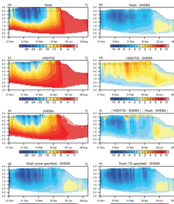
The evolution of snow and sea ice temperature observed at Pittsburgh and simulated by Noah and HIGHTSI can be inferred from Fig. 2. Both Noah and HIGHTSI can simu-late the annual cycle of the sea ice temperature well. A cold bias is observed in the simulation by Noah when the sea ice grows thicker and a warm bias is observed when the sea ice
becomes thinner. The bias in Noah increases from the be-ginning of the simulation and becomes the largest in winter. It is colder than the SHEBA observations and the bias can reach−10◦C in the upper part of the sea ice in December and January. The snow depth is well simulated by HIGHTSI, while it is overestimated by Noah. This is because Noah fixes the snow density at a value (300 kg m−3) smaller than that (320 kg m−3) recommended by SIMIP2. The ablation pro-cesses like blowing snow are also neglected in Noah. We performed a sensitivity experiment in which the snow depth in Noah is specified based on the SHEBA observations. The bias still exists in this simulation, implying that the over-estimation of snow depth does not play a role in the bias of sea ice temperature. Another experiment based on Noah is performed to determine to what extent the turbulent flux and albedo may contribute to the bias. In this simulation, the Noah sea ice model does not calculate turbulent fluxes and the surface temperature is specified based on the SHEBA observations. However, the bias in sea ice temperature still exists, and the bias in the upper part of the sea ice is over 6◦C during winter. Such a bias exists when the temperature of both the upper and lower boundary of the sea ice is fixed at the observational value, which means that the error is as-sociated with energy imbalance within the sea ice. The sea ice temperature simulated by HIGHTSI, on the other hand, is warmer than the SHEBA observations during early spring. During other times of the year, the bias in the temperature simulation is rather small in HIGHTSI.
energy-Figure 2.The evolution of sea ice temperature: results from(a)Noah,(c)HIGHTSI and(e)SHEBA observation; bias of(b)Noah,(d) HIGH-TSI,(g)Noah with specified snow depth on sea ice and(h)Noah with specified snow depth and surface temperature on sea ice; and(f)the difference between the absolute bias of HIGHTSI and SHEBA.
conservative method (Launiainen and Cheng, 1998). At each integration step, the thickness of the uppermost and the bot-tom layer of ice changes when ablation or accretion happens. Then an integral interpolation method which can ensure the conservation of heat is utilized to remap the ice tempera-ture to the standard sigma levels. In Noah, however, imbal-ance of energy in sea ice happens when it is specified with a time-dependent ice thickness. Without a remapping step like that in HIGHTSI, the temperature at each sigma level in Noah would not change although the sigma level is ac-tually representing a different depth after the change in ice thickness. Such a problem of energy imbalance imposes a pseudo-cooling effect when the ice grows thicker in winter and a pseudo-warming effect when the ice becomes thinner in summer.
4 Validation of the online simulation
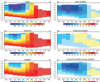
Figure 3.The evolution of monthly mean sea ice temperature: results from(a)Noah,(c)HIGHTSI and(e)SHEBA observation; bias of (b)Noah and(d)HIGHTSI; and(f)the difference between the absolute bias of HIGHTSI and SHEBA.
us to evaluate the model’s performance over different types of sea ice.
Because climate simulation is studied here, the model was freely integrated from 1 October 1997 to 1 Novem-ber 1998 without any reinitialization during the simulation. This caused our results to differ from those in Bromwich et al. (2009), which reinitialized the model every 24 h from the ERA40 reanalysis. The initial and lateral boundary con-ditions are provided by ERA-Interim reanalysis, and the sea surface temperature (SST) and sea ice concentration are pro-vided by the National Oceanic and Atmospheric Administra-tion (NOAA) Optimal InterpolaAdministra-tion SST analysis (OISST) version 2 and the National Aeronautics and Space Admin-istration (NASA) bootstrap, respectively (Reynolds et al., 2002; Comiso and Nishio, 2008). The resolution of OISST is 0.25◦, and that of NASA bootstrap is 25 km, which is close to the resolution of our simulation. The initial condi-tion of snow depth on sea ice is provided by the Pan-Arctic Ice-Ocean Modeling and Assimilation system (Zhang and Rothrock, 2003, PIOMAS), a reanalysis product with a res-olution of approximately 25 km. PIOMAS also provides the field of ocean heat flux which is essential for the calculation of basal accretion and ablation.
In this study, the sea ice thickness in both WRF-Noah and WRF-HIGHTSI is updated every day by the PIOMAS prod-ucts. The sea ice thickness from PIOMAS exhibits a similar pattern to observations (Laxon et al., 2013), and it has already
been used as a boundary condition for simulations using the WRF model (Hines et al., 2015). It should be noted that al-though the ice thickness in WRF-HIGHTSI is specified with reanalysis data, the sea ice component still includes the ice ablation and accretion processes. The integral interpolation method which is energy-conservative is utilized at each inte-gration step. Since the ice thickness at each grid may change due to the drift of sea ice, only including the thermodynamic effect is not enough for a realistic simulation of ice thickness. The simulation of sea ice thickness change may be biased when the lateral flux of ice mass is neglected. To reduce this bias, the PIOMAS data are applied to correct the ice thick-ness after HIGHTSI has calculated the ablation and accre-tion of sea ice. In this way, the energy is not conservative for sea ice simulation in WRF-HIGHTSI. However, this prob-lem of energy imbalance is smaller than that in WRF-Noah since WRF-HIGHTSI has taken the thickness change that is related with thermodynamic processes into consideration.
-
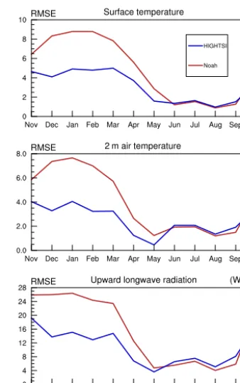
-Figure 4.Monthly mean surface temperature, 2 m air temperature and surface upward long-wave and shortwave radiation simulated and observed at the SHEBA sites.
The results in this study were based on version 3.6.1 of the polar-modified WRF model, which was the latest release at the time of this study. For the choice of parameterization schemes, we used the same set as most of those used in the Arctic System Reanalysis (Bromwich et al., 2015). Kain– Fritsch cumulus (Kain, 2004), Mellor–Yamada–Nakanishi– Niino 2.5-level planetary boundary layer (Nakanish, 2001), Morrison two-moments microphysics (Morrison et al., 2009) and Noah land surface are used for the parameterization schemes in our simulation (Chen and Dudhia, 2001). For long-wave and shortwave radiation, we use climate model-ready updates to the Rapid Radiative Transfer Model known as RRTMG (Iacono et al., 2008).
The 6-hourly outputs from the simulation are bilinearly in-terpolated to the point where the SHEBA station was located at each time. Then, the monthly averages of the SHEBA observations and model results are compared. Considering the sea ice temperature (Fig. 3), cold biases remain in both WRF-Noah and WRF-HIGHTSI in the upper part of the sea ice during winter. Such a cold bias in WRF-Noah can reach
−10◦C. In summer, both WRF-Noah and WRF-HIGHTSI show smaller biases. In accordance with the results from offline simulations, WRF-Noah tends to underestimate the sea ice temperature when the ice grows thicker, and overes-timate the sea ice temperature when the ice becomes thin-ner. As has been found in the offline simulation, this bias is mainly caused by a problem of energy imbalance in ice. The bias becomes smaller near the bottom part of the sea ice, since the temperature at the lower bound of sea ice is fixed at the freezing point of seawater. Benefiting from inclu-sion of the ablation and accretion processes, WRF-HIGHTSI can better resolve the energy balance in sea ice. The bias of sea ice temperature simulated by WRF-HIGHTSI is consid-erably smaller than WRF-Noah during December to March when the ice grows thicker.
-Figure 5.Surface temperature, 2 m air temperature and surface upward long-wave radiation over sea ice surface in January 1998: observations and bias in Noah and HIGHTSI.
The surface air temperatures (at heights of 2.5 m for SHEBA observations and 2 m for ERA-Interim and WRF) simulated in WRF and ERA-Interim are also evaluated. Ben-efiting from the data assimilation, the results from ERA-Interim are the closest with respect to the SHEBA obser-vation. Both WRF-Noah and WRF-HIGHTSI underestimate the surface air temperature, whereas WRF-HIGHTSI has a smaller bias than WRF-Noah by about 5◦C in winter. Simi-lar to the simulation of surface temperature, WRF-Noah un-derestimates the surface upward long-wave radiation dur-ing winter. WRF-HIGHTSI, on the other hand, has better performance in simulating the upward long-wave radiation than WRF-Noah due to the better representation of the sur-face temperature. WRF-HIGHTSI reduces the bias by about 20 W m−2in winter. Due to the smaller vertical gradient of sea ice temperature in summer, the bias becomes smaller for
a relationship between sea ice albedo and surface temper-ature which is sensitive to tunable parameters. The sea ice albedo simulated by Noah is based on an empirical relation-ship derived from the SHEBA observations (Bromwich et al., 2009), and this estimation has been shown to give a result close to the SHEBA observations (Porter et al., 2011). Due to the high albedo of sea ice surface, most of the downward shortwave radiation would be reflected back to the air. This means the upward shortwave radiation can be strongly in-fluenced by the incoming amount. As mentioned above, the misrepresentation of cloud radiative effect leads to the under-estimation of downward shortwave radiation from air to the surface. This underestimation of surface incoming shortwave radiation would reduce the reflected amount as simulated by both WRF-Noah and WRF-HIGHTSI. Such a bias in upward shortwave radiation simulated by WRF-HIGHTSI is partly compensated by its overestimation of the sea ice albedo.
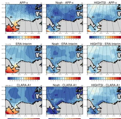
In addition to the verification at the SHEBA site, the evalu-ation is also conducted over the entire domain covered by sea ice. Figure 5 shows the surface temperature, 2 m air temper-ature and surface upward long-wave radiation from observa-tions and their biases from WRF-Noah and WRF-HIGHTSI on January 1998. With reference to the satellite observation, the cold bias in simulating the surface temperature found at the SHEBA site can be observed anywhere that is covered by sea ice. The pattern of the bias in simulating the surface temperature was consistent with those in simulating the 2 m air temperature and surface upward long-wave radiation. The biases were considerably smaller in WRF-HIGHTSI than in WRF-Noah over all the grid points covered by sea ice. A summary of the performance of HIGHTSI, WRF-Noah and ERA-Interim in simulating the surface tempera-ture and radiation budget is given in terms of the metric as a root-mean-squared error (RMSE) with respect to observa-tions (Fig. 6). In general, the RMSE was larger in winter than in summer, and WRF-HIGHTSI had a significantly smaller RMSE than WRF-Noah in winter.
5 Impact of the sea ice thickness specification
Previous studies have shown that sea ice thickness exerts an indiscernible influence on the atmosphere over sea ice (Gerdes, 2006; Krinner et al., 2009; Day et al., 2014). It has been acknowledged that prescribing the sea ice fraction alone might lead to bias in the simulation of surface energy balance, particularly over the seasonal sea ice. To fulfill this demand, the ability to prescribe the observed sea ice thick-ness and the sea ice fraction is added to the recent versions of the WRF and Polar WRF models. Due to the difficulties in observing and retrieving the sea ice thickness, routinely reliable observations were not available at the time of this study. Some reanalysis products (such as PIOMAS used in this study) have provided useful information on the sea ice thickness with high spatial and temporal resolutions.
How
-Figure 6.RMSE of surface temperature, 2 m air temperature and upward long-wave radiation for WRF-Noah and WRF-HIGHTSI.
ever, note that the limited observations in the assimilation system can impact the quality of the sea ice reanalyses. Ad-ditionally, the surface energy imbalance could result from the inconsistency between the different sea ice in the reanalysis and that in the regional climate model. Currently, there are three ways to prescribe the sea ice thickness in the regional atmospheric model: treating sea ice as a constant value every-where, using the spatially and temporally variant values from observations or reanalyses, or applying a simple parameteri-zation based on the knowledge of the statistical relationship between sea ice thickness and sea ice fraction. The simple pa-rameterization of sea ice thickness is represented in the form as the following equation, as first proposed by Krinner et al. (1997).
d= 0.2+3.8 fmin2 (1+2(f−fmin)) (1)
Hered denotes the sea ice thickness,f denotes the sea ice fraction, andfmin denotes the minimum sea ice fraction at
that grid point. The sea ice thickness estimated from this empirical method has proven to show a similar pattern with the observational value in both Arctic and Antarctic sea ice in terms of the climatological mean. However, the seasonal variation of ice thickness cannot be realistically represented by the estimation based only on sea ice fraction.
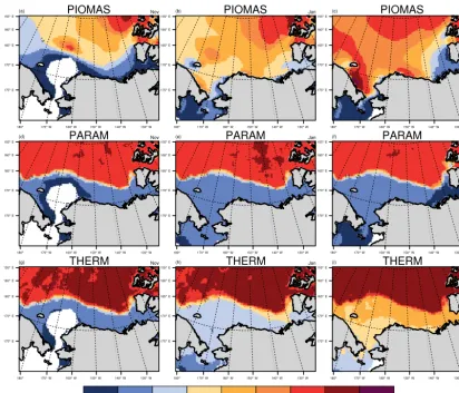
Figure 7.Sea ice thickness in PIOMAS, PARAM and THERM during November 1997, January 1998 and May 1998.
as in the simple parameterization and the potential ability of a complex thermodynamic sea ice model to predict the change in sea ice thickness. During the climate simulation of the regional climate model (WRF-HIGHTSI in this study), the sea ice thickness estimated from Eq. (1) is used as the initial value when no sea ice is presented in the previous time step. Along with the integration of the RCM, the change in sea ice thickness is determined by the HIGHTSI component. For the grid point where no sea ice is present in the previous time step, the sea ice thickness is also prescribed from Eq. (1) as an initial guess. In this way, the evolution of sea ice thick-ness is somewhat more reasonable than the value obtained only from the empirical method because the thermodynamic air–ice interaction could be resolved in RCM, and a seasonal variation of ice thickness can be introduced by including the ablation and accretion processes.
To test the impact of sea ice specification, three more sim-ulations are performed to compare the simsim-ulations with dif-ferent treatments of sea ice thickness. One simulation uses the same model as WRF-Noah in the previous section, but fixes the sea ice thickness at 3 m (hereafter referred to as
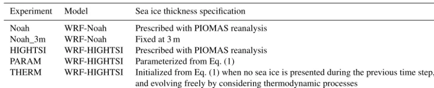
Table 2.Experiment setup for studying the impact of the sea ice thickness specification
Experiment Model Sea ice thickness specification
Noah WRF-Noah Prescribed with PIOMAS reanalysis Noah_3m WRF-Noah Fixed at 3 m
HIGHTSI WRF-HIGHTSI Prescribed with PIOMAS reanalysis PARAM WRF-HIGHTSI Parameterized from Eq. (1)
THERM WRF-HIGHTSI Initialized from Eq. (1) when no sea ice is presented during the previous time step, and evolving freely by considering thermodynamic processes
influences the initial guess and the ice thickness is allowed to be evolved freely based on the calculation by HIGHTSI.
The sea ice thickness from the PIOMAS, the empirical es-timation in PARAM and the results from THERM are pre-sented in Fig. 7. Based on the results from PARAM, the perennial sea ice was approximately 3 m thick and the sea-sonal sea ice was less than 1 m thick. This empirical esti-mation could, to some extent, mimic the general climatol-ogy characteristics of the thickness distribution, whereas it could not provide detailed information spatially and tempo-rally. The PARAM overestimates the perennial sea ice thick-ness throughout the year while it underestimates the seasonal sea ice thickness in winter and spring. Within the simula-tion domain in this study, the perennial sea ice thickness as shown in PIOMAS is around 2 m in November and is about 2.5 m thick in May. The 3 m ice thickness for perennial sea ice as estimated from Eq. (1) is thicker than the PIOMAS re-sult. For the seasonal sea ice, a thickening trend during win-tertime could be found based on the PIOMAS result. The estimation from Eq. (1) could not introduce such a thick-ening trend since the sea ice fraction is already near 1 at each grid point. This is the limitation of the empirical esti-mation for ice thickness. Based on the results from THERM, the sea ice thickness was similar to that from the PARAM when the model-free run had just begun. Thus, it shared the same bias with that in PARAM. Benefiting from the consid-eration of accretion process of sea ice, the thickening trend of sea ice thickness during wintertime could be introduced in THERM. This thickening trend would enlarge the posi-tive bias of perennial sea ice thickness as the initial guess had already overestimated the ice thickness. The perennial sea ice thickness as simulated by THERM was over 4 m in May, which was much thicker than the estimation from PI-OMAS. Despite of the systematic overestimation, the ten-dency of thickness change for perennial sea ice as simu-lated by THERM was close to that from PIOMAS. Thus a better simulation of perennial sea ice thickness might be possible given a more realistic initial guess. The thickening tendency that was introduced onto the seasonal sea ice en-abled THERM to simulate a thicker seasonal sea ice than PARAM during wintertime. For seasonal sea ice, the initial guess given by empirical estimation is close to the observa-tion during the beginning of the simulaobserva-tion. When the sea ice
grows thicker, THERM would introduce the thickening trend which was lacking in PARAM. THERM simulates a seasonal sea ice over Chukchi Sea and Beaufort Sea during wintertime thicker than PARAM, which is closer to the observation. De-tailed spatial features of change in sea ice thickness could not be fully resolved in THERM because it could not ac-count for the dynamic sea ice processes. For example, both the thermodynamic and dynamic processes over the Bering Sea would play an important role and could show opposite signs and nearly cancel each other (Li et al., 2014). Lacking the influence of ice motion, THERM simulated a continuous thickening trend of sea ice over Bering Sea during winter. This leads to a positive bias of about 1 m for the ice thick-ness in May. Consequently, the THERM method could rep-resent the seasonal evolution of sea ice thickness, but it would also depend on the initial guess that was estimated from the empirical parameterization. In our simulation, the THERM method showed better results than PARAM over seasonal sea ice, while it led to a larger bias over perennial sea ice.
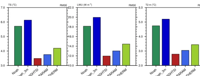
-Figure 8.RMSE of surface temperature, upward long-wave radiation and 2 m air temperature for WRF-Noah and WRF-HIGHTSI prescribed with different sea ice thicknesses.
6 Conclusions
As a major feature in the polar climate system, sea ice plays an important role in the air–ice–ocean interaction and needs to be properly represented in polar RCMs. The WRF model, which has been widely used in polar research, applies the Noah scheme as its only option for sea ice simulation. Previ-ous research has shown that the simplification in the Noah sea ice model can lead to problems of energy imbalance when used for polar climate simulation (Valkonen et al., 2014). HIGHTSI, a complex thermodynamic sea ice model, shows advantages over Noah in several aspects. HIGHTSI has a higher resolution for both snow and ice than Noah, and it takes into account the penetration of solar energy in ice layers. Moreover, HIGHTSI includes the ice ablation and accretion processes and uses an interpolation method which can ensure heat conservation during each integration step. These features enable HIGHTSI to better resolve the en-ergy balance in the sea ice than Noah. Forced with atmo-spheric conditions observed during the SHEBA experiment, Noah sea ice exhibits a cold bias which can reach−10◦C during winter when simulating the sea ice temperature. This bias still exists when the snow depth and surface tempera-ture in Noah are specified with observations, indicating that the bias in Noah is associated with energy imbalance within sea ice. When prescribed with a time-dependent ice thick-ness, a lack of the interpolation step which can ensure the conservation of heat would lead to a cold bias when the ice grows thicker and a warm bias when the ice becomes thin-ner. HIGHTSI, which overcomes this shortage by resolving the energy balance in ice, provides a better simulation than Noah. The cold bias of sea ice temperature in Noah is sig-nificantly reduced in HIGHTSI. To determine the possible added value from a complex thermodynamic sea ice model, HIGHTSI is coupled into the polar-modified WRF model. Benefiting from the better representation of energy balance in ice as shown in the offline simulation, the WRF model coupled with HIGHTSI (WRF-HIGHTSI) significantly re-duced the bias in simulating the sea ice temperature than
the original Polar WRF which uses Noah (WRF-Noah). This leads to a better representation of the surface temperature, surface upward long-wave radiation and 2 m air temperature in the WRF-HIGHTSI compared with WRF-Noah. Consid-ering the bias with reference to SHEBA observations, WRF-HIGHTSI improves the simulation of surface temperature, 2 m air temperature and surface upward long-wave radiation flux in winter by 6, 5◦C and 20 W m−2, respectively.
The appropriate specification of sea ice thickness is im-portant for climate simulations in the polar region. Regional climate simulations with sea ice thickness prescribed by dif-ferent methods are conducted to study the impact from differ-ent treatmdiffer-ents of sea ice thickness. Consistdiffer-ent with previous studies (Hines et al., 2015), prescribing the sea ice thickness with observational information results in the best simulation among all the other methods. If no observational informa-tion is available, using an empirical method based on the re-lationship between sea ice concentration and sea ice thick-ness could, to some extent, mimic the large-scale feature of the thickness distribution. However, this empirical estimation can not account for spatial details and the seasonal variation of ice thickness. In this study, we test another method to see how the sea ice thickness would be simulated given a com-plex thermodynamic sea ice model which includes the abla-tion and accreabla-tion processes. This method initializes the sea ice thickness from the empirical estimation, while the further change in ice thickness is predicted by the thermodynamic sea ice model itself. Based on this method, the tendency of seasonal change in sea ice thickness can be introduced. How-ever, the ice thickness simulated through this method de-pends much on the quality of the initial guess of ice thickness and the role of the ice dynamic processes. As a result, spec-ifying ice thickness from other sources like PIOMAS would still be the best practice for climate simulation based on cur-rent atmospheric-only RCMs.
However, a lack of sea ice dynamic processes means that the horizontal transport of mass and energy in sea ice is ignored in the regional atmospheric model. To account for this prob-lem, sea ice thickness from PIOMAS reanalysis is used in this study. This means the simulation of sea ice will rely on the driving field of ice thickness, and the air–ice–ocean in-teraction in the polar climate system could not be fully rep-resented. Therefore, although the development of coupled RCM is still a challenging task, it is an essential pathway toward a realistic simulation of the polar climate (Berg et al., 2015).
7 Code availability
The source code of WRF-HIGHTSI can be obtained at https: //github.com/yaoraistlin/WRF-HIGHTSI.
Acknowledgements. This work is supported by the National Basic Research Program of China (2013CBA01805), the National Natu-ral Science Foundation for Young Scientists of China (41305054) and Tsinghua University Initiative Scientific Research Program (20131089356). Our work is completed on the Explorer 100 cluster system of Tsinghua National Laboratory for Information Science and Technology.
Edited by: J. Annan
References
Andreas, E. L., Persson, P. O. G., Grachev, A. A., Jordan, R. E., Horst, T. W., Guest, P. S., and Fairall, C. W.: Parameterizing Tur-bulent Exchange over Sea Ice in Winter, J. Hydrometeorol., 11, 87–104, doi:10.1175/2009jhm1102.1, 2010.
Barton, N. P., Klein, S. A., and Boyle, J. S.: On the Contribu-tion of Longwave RadiaContribu-tion to Global Climate Model Biases in Arctic Lower Tropospheric Stability, J. Climate, 27, 7250–7269, doi:10.1175/jcli-d-14-00126.1, 2014.
Berg, P., Döscher, R., and Koenigk, T.: On the effects of con-straining atmospheric circulation in a coupled atmosphere-ocean Arctic regional climate model, Clim. Dynam., 46, 3499–3515, doi:10.1007/s00382-015-2783-y, 2015.
Bourassa, M. A., Gille, S. T., Bitz, C., Carlson, D., Cerovecki, I., Clayson, C. A., Cronin, M. F., Drennan, W. M., Fairall, C. W., Hoffman, R. N., Magnusdottir, G., Pinker, R. T., Ren-frew, I. A., Serreze, M., Speer, K., Talley, L. D., and Wick, G. A.: High-Latitude Ocean and Sea Ice Surface Fluxes: Chal-lenges for Climate Research, B. Am. Meteorol. Soc., 94, 403– 423, doi:10.1175/bams-d-11-00244.1, 2013.
Bromwich, D. H., Hines, K. M., and Bai, L.-S.: Development and testing of Polar Weather Research and Forecasting model: 2. Arctic Ocean, J. Geophys. Res.-Atmos., 114, D08122, doi:10.1029/2008JD010300, 2009.
Bromwich, D. H., Otieno, F. O., Hines, K. M., Manning, K. W., and Shilo, E.: Comprehensive evaluation of polar weather research and forecasting model performance in the Antarctic, J. Geophys. Res.-Atmos., 118, 274–292, doi:10.1029/2012jd018139, 2013.
Bromwich, D. H., Wilson, A. B., Bai, L.-S., Moore, G. W. K., and Bauer, P.: A comparison of the regional Arctic System Reanaly-sis and the global ERA-Interim ReanalyReanaly-sis for the Arctic, Q. J. Roy. Meteor. Soc., 142, 644–658, doi:10.1002/qj.2527, 2015. Cassano, J. J., Higgins, M. E., and Seefeldt, M. W.: Performance of
the Weather Research and Forecasting Model for Month-Long Pan-Arctic Simulations, Mon. Weather Rev., 139, 3469–3488, doi:10.1175/mwr-d-10-05065.1, 2011.
Chen, F. and Dudhia, J.: Coupling an Advanced Land Surface– Hydrology Model with the Penn State–NCAR MM5 Mod-eling System. Part I: Model Implementation and Sensitiv-ity, Mon. Weather Rev., 129, 569–585, doi:10.1175/1520-0493(2001)129<0569:caalsh>2.0.co;2, 2001.
Cheng, B., Vihma, T., Pirazzini, R., and Granskog, M. A.: Modelling of superimposed ice formation during the spring snowmelt period in the Baltic Sea, Ann. Glaciol., 44, 139–146, doi:10.3189/172756406781811277, 2006.
Cheng, B., Vihma, T., Zhang, Z.-h., Zhi-jun, L., and Hui-ding, W.: Snow and sea ice thermodynamics in the Arctic: Model valida-tion and sensitivity study against SHEBA data, Chinese Journal of Polar Science, 19, 108–122, 2008a.
Cheng, B., Zhang, Z., Vihma, T., Johansson, M., Bian, L., Li, Z., and Wu, H.: Model experiments on snow and ice thermodynamics in the Arctic Ocean with CHINARE 2003 data, J. Geophys. Res.-Oceans, 113, C09020, doi:10.1029/2007JC004654, 2008b. Cheng, B., Mäkynen, M., Similä, M., Rontu, L., and Vihma,
T.: Modelling snow and ice thickness in the coastal Kara Sea, Russian Arctic, Ann. Glaciol., 54, 105–113, doi:10.3189/2013aog62a180, 2013.
Collins, W. D., Bitz, C. M., Blackmon, M. L., Bonan, G. B., Bretherton, C. S., Carton, J. A., Chang, P., Doney, S. C., Hack, J. J., Henderson, T. B., Kiehl, J. T., Large, W. G., McKenna, D. S., Santer, B. D., and Smith, R. D.: The Community Climate System Model Version 3 (CCSM3), J. Climate, 19, 2122–2143, doi:10.1175/jcli3761.1, 2006.
Comiso, J. C. and Nishio, F.: Trends in the sea ice cover using en-hanced and compatible AMSR-E, SSM/I, and SMMR data, J. Geophys. Res., 113, C02S07, doi:10.1029/2007jc004257, 2008. Curry, J. A. and Lynch, A. H.: Comparing Arctic Regional Climate Model, Eos T. Am. Geophys. Un., 83, 87–87, doi:10.1029/2002EO000051, 2002.
Day, J. J., Hawkins, E., and Tietsche, S.: Will Arctic sea ice thick-ness initialization improve seasonal forecast skill?, Geophys. Res. Lett., 41, 7566–7575, doi:10.1002/2014GL061694, 2014. Dorn, W., Dethloff, K., and Rinke, A.: Improved simulation of
feed-backs between atmosphere and sea ice over the Arctic Ocean in a coupled regional climate model, Ocean Model., 29, 103–114, doi:10.1016/j.ocemod.2009.03.010, 2009.
Dorn, W., Dethloff, K., and Rinke, A.: Limitations of a coupled regional climate model in the reproduction of the observed Arctic sea-ice retreat, The Cryosphere, 6, 985–998, doi:10.5194/tc-6-985-2012, 2012.
Dupont, F., Vancoppenolle, M., Tremblay, L.-B., and Huwald, H.: Comparison of different numerical approaches to the 1D sea-ice thermodynamics problem, Ocean Model., 87, 20–29, doi:10.1016/j.ocemod.2014.12.006, 2015.
CMIP5 Models, J. Climate, 28, 6019–6038, doi:10.1175/jcli-d-14-00801.1, 2015.
Fréville, H., Brun, E., Picard, G., Tatarinova, N., Arnaud, L., Lan-conelli, C., Reijmer, C., and van den Broeke, M.: Using MODIS land surface temperatures and the Crocus snow model to under-stand the warm bias of ERA-Interim reanalyses at the surface in Antarctica, The Cryosphere, 8, 1361–1373, doi:10.5194/tc-8-1361-2014, 2014.
Gerdes, R.: Atmospheric response to changes in Arc-tic sea ice thickness, Geophys. Res. Lett., 33, L18709, doi:10.1029/2006gl027146, 2006.
Glisan, J. M. and Gutowski, W. J.: WRF summer extreme daily pre-cipitation over the CORDEX Arctic, J. Geophys. Res.-Atmos., 119, 1720–1732, doi:10.1002/2013jd020697, 2014a.
Glisan, J. M. and Gutowski, W. J.: WRF winter extreme daily precipitation over the North American CORDEX Arctic, J. Geophys. Res.-Atmos., 119, 10738–10748, doi:10.1002/2014JD021676, 2014b.
Hines, K. M. and Bromwich, D. H.: Development and Testing of Polar Weather Research and Forecasting (WRF) Model. Part I: Greenland Ice Sheet Meteorology, Mon. Weather Rev., 136, 1971–1989, doi:10.1175/2007mwr2112.1, 2008.
Hines, K. M., Bromwich, D. H., Bai, L.-S., Barlage, M., and Slater, A. G.: Development and Testing of Polar WRF. Part III: Arctic Land, J. Climate, 24, 26–48, doi:10.1175/2010jcli3460.1, 2011. Hines, K. M., Bromwich, D. H., Bai, L., Bitz, C. M., Powers,
J. G., and Manning, K. W.: Sea Ice Enhancements to Polar WRF, Mon. Weather Rev., 143, 2363–2385, doi:10.1175/MWR-D-14-00344.1, 2015.
Huwald, H., Tremblay, L.-B., and Blatter, H.: Reconciling different observational data sets from Surface Heat Budget of the Arc-tic Ocean (SHEBA) for model validation purposes, J. Geophys. Res.-Oceans, 110, C05009, doi:10.1029/2003JC002221, 2005. Iacono, M. J., Delamere, J. S., Mlawer, E. J., Shephard, M. W.,
Clough, S. A., and Collins, W. D.: Radiative forcing by long-lived greenhouse gases: Calculations with the AER ra-diative transfer models, J. Geophys. Res., 113, D13103, doi:10.1029/2008jd009944, 2008.
Jin, Z., Stamnes, K., Weeks, W. F., and Tsay, S.-C.: The effect of sea ice on the solar energy budget in the atmosphere-sea ice-ocean system: A model study, J. Geophys. Res.-Oceans, 99, 25281– 25294, doi:10.1029/94JC02426, 1994.
Jones, P. D. and Lister, D. H.: Antarctic near-surface air tempera-tures compared with ERA-Interim values since 1979, Int. J. Cli-matol., 35, 1354–1366, doi:10.1002/joc.4061, 2014.
Kain, J. S.: The Kain–Fritsch Convective Parameterization: An Update, J. Appl. Meteorol., 43, 170–181, doi:10.1175/1520-0450(2004)043<0170:tkcpau>2.0.co;2, 2004.
Karlsson, J. and Svensson, G.: Consequences of poor representation of Arctic sea-ice albedo and cloud-radiation interactions in the CMIP5 model ensemble, Geophys. Res. Lett., 40, 4374–4379, doi:10.1002/grl.50768, 2013.
Karlsson, K.-G., Riihelä, A., Müller, R., Meirink, J. F., Sedlar, J., Stengel, M., Lockhoff, M., Trentmann, J., Kaspar, F., Hollmann, R., and Wolters, E.: CLARA-A1: a cloud, albedo, and radiation dataset from 28 yr of global AVHRR data, Atmos. Chem. Phys., 13, 5351–5367, doi:10.5194/acp-13-5351-2013, 2013.
Karvonen, J., Cheng, B., Vihma, T., Arkett, M., and Carrieres, T.: A method for sea ice thickness and concentration analysis based
on SAR data and a thermodynamic model, The Cryosphere, 6, 1507–1526, doi:10.5194/tc-6-1507-2012, 2012.
Key, J. R., Collins, J. B., Fowler, C., and Stone, R. S.: High-latitude surface temperature estimates from thermal satellite data, Remote Sens. Environ., 61, 302–309, doi:10.1016/S0034-4257(97)89497-7, 1997.
Koenigk, T., Devasthale, A., and Karlsson, K.-G.: Summer Arctic sea ice albedo in CMIP5 models, Atmos. Chem. Phys., 14, 1987– 1998, doi:10.5194/acp-14-1987-2014, 2014.
Koenigk, T., Berg, P., and Döscher, R.: Arctic climate change in an ensemble of regional CORDEX simulations, Polar Res., 34, 24603, doi:10.3402/polar.v34.24603, 2015.
Krinner, G., Genthon, C., Li, Z.-X., and Le Van, P.: Studies of the Antarctic climate with a stretched-grid general circu-lation model, J. Geophys. Res.-Atmos., 102, 13731–13745, doi:10.1029/96JD03356, 1997.
Krinner, G., Rinke, A., Dethloff, K., and Gorodetskaya, I. V.: Im-pact of prescribed Arctic sea ice thickness in simulations of the present and future climate, Clim. Dynam., 35, 619–633, doi:10.1007/s00382-009-0587-7, 2009.
Launiainen, J. and Cheng, B.: Modelling of ice thermodynamics in natural water bodies, Cold Reg. Sci. Technol., 27, 153–178, 1998.
Laxon, S. W., Giles, K. A., Ridout, A. L., Wingham, D. J., Willatt, R., Cullen, R., Kwok, R., Schweiger, A., Zhang, J., Haas, C., Hendricks, S., Krishfield, R., Kurtz, N., Farrell, S., and Davidson, M.: CryoSat-2 estimates of Arctic sea ice thickness and volume, Geophys. Res. Lett., 40, 732–737, doi:10.1002/grl.50193, 2013. Li, L., Miller, A. J., McClean, J. L., Eisenman, I., and Hen-dershott, M. C.: Processes driving sea ice variability in the Bering Sea in an eddying ocean/sea ice model: anomalies from the mean seasonal cycle, Ocean Dynam., 64, 1693–1717, doi:10.1007/s10236-014-0769-7, 2014.
Liu, F., Krieger, J. R., and Zhang, J.: Toward Producing the Chukchi–Beaufort High-Resolution Atmospheric Reanalysis (CBHAR) via the WRFDA Data Assimilation System, Mon. Weather Rev., 142, 788–805, 2014.
Morrison, H., Thompson, G., and Tatarskii, V.: Impact of Cloud Microphysics on the Development of Trailing Stratiform Pre-cipitation in a Simulated Squall Line: Comparison of One- and Two-Moment Schemes, Mon. Weather Rev., 137, 991–1007, doi:10.1175/2008mwr2556.1, 2009.
Nakanish, M.: Improvement Of The Mellor-Yamada Turbulence Closure Model Based On Large-Eddy Simulation Data, Bound.-Lay. Meteorol., 99, 349–378, doi:10.1023/a:1018915827400, 2001.
Notz, D.: Challenges in simulating sea ice in Earth System Mod-els, WIREs Climatic Change, 3, 509–526, doi:10.1002/wcc.189, 2012.
Perovich, D. K. and Elder, B. C.: Temporal evolution of Arctic sea-ice temperature, Ann. Glaciol., 33, 207–211, doi:10.3189/172756401781818158, 2001.
Pithan, F., Medeiros, B., and Mauritsen, T.: Mixed-phase clouds cause climate model biases in Arctic wintertime temperature in-versions, Clim. Dynam., 43, 289–303, doi:10.1007/s00382-013-1964-9, 2013.
reanalyses and satellite observations, J. Geophys. Res.-Atmos., 116, D22108, doi:10.1029/2011JD016622, 2011.
Reynolds, R. W., Rayner, N. A., Smith, T. M., Stokes, D. C., and Wang, W.: An Improved In Situ and Satellite SST Analy-sis for Climate, J. Climate, 15, 1609–1625, doi:10.1175/1520-0442(2002)015<1609:aiisas>2.0.co;2, 2002.
Riihelä, A., Manninen, T., and Laine, V.: Observed changes in the albedo of the Arctic sea-ice zone for the period 1982–2009, Nature Climate Change, 3, 895–898, doi:10.1038/nclimate1963, 2013.
Rinke, A., Maslowski, W., Dethloff, K., and Clement, J.: Influence of sea ice on the atmosphere: A study with an Arctic atmo-spheric regional climate model, J. Geophys. Res., 111, D16103, doi:10.1029/2005jd006957, 2006.
Semmler, T., Cheng, B., Yang, Y., and Rontu, L.: Snow and ice on Bear Lake (Alaska) a sensitivity experiments with two lake ice models, Tellus A, 64, 17339, doi:10.3402/tellusa.v64i0.17339, 2012.
Sorteberg, A., Kattsov, V., Walsh, J. E., and Pavlova, T.: The Arc-tic surface energy budget as simulated with the IPCC AR4 AOGCMs, Clim. Dynam., 29, 131–156, doi:10.1007/s00382-006-0222-9, 2007.
Steeneveld, G. J., van de Wiel, B. J. H., and Holtslag, A. A. M.: Modeling the Evolution of the Atmospheric Boundary Layer Coupled to the Land Surface for Three Contrasting Nights in CASES-99, J. Atmos. Sci., 63, 920–935, doi:10.1175/jas3654.1, 2006.
Sterk, H. A. M., Steeneveld, G. J., and Holtslag, A. A. M.: The role of snow-surface coupling, radiation, and turbulent mixing in modeling a stable boundary layer over Arctic sea ice, J. Geophys. Res.-Atmos., 118, 1199–1217, doi:10.1002/jgrd.50158, 2013. Svensson, G. and Karlsson, J.: On the Arctic Wintertime
Cli-mate in Global CliCli-mate Models, J. CliCli-mate, 24, 5757–5771, doi:10.1175/2011jcli4012.1, 2011.
Tjernström, M., Sedlar, J., and Shupe, M. D.: How Well Do Re-gional Climate Models Reproduce Radiation and Clouds in the Arctic? An Evaluation of ARCMIP Simulations, J. Appl. Meteo-rol. Clim., 47, 2405–2422, doi:10.1175/2008jamc1845.1, 2008. Uttal, T., Curry, J. A., Mcphee, M. G., Perovich, D. K., Moritz,
R. E., Maslanik, J. A., Guest, P. S., Stern, H. L., Moore, J. A., Turenne, R., Heiberg, A., Serreze, M. C., Wylie, D. P., Pers-son, O. G., PaulPers-son, C. A., Halle, C., MoriPers-son, J. H., Wheeler, P. A., Makshtas, A., Welch, H., Shupe, M. D., Intrieri, J. M., Stamnes, K., Lindsey, R. W., Pinkel, R., Pegau, W. S., Stanton, T. P., and Grenfeld, T. C.: Surface Heat Budget of the Arctic Ocean, B. Am. Meteorol. Soc., 83, 255–275, doi:10.1175/1520-0477(2002)083<0255:shbota>2.3.co;2, 2002.
Valkonen, T., Vihma, T., Johansson, M. M., and Launiainen, J.: Atmosphere–sea ice interaction in early summer in the Antarctic: evaluation and challenges of a regional atmospheric model, Q. J. Roy. Meteor. Soc., 140, 1536–1551, doi:10.1002/qj.2237, 2014. Vihma, T. and Pirazzini, R.: On the Factors Controlling the
Snow Surface and 2-m Air Temperatures Over the Arc-tic Sea Ice in Winter, Bound.-Lay. Meteorol., 117, 73–90, doi:10.1007/s10546-004-5938-7, 2005.
Vihma, T., Uotila, J., Cheng, B., and Launiainen, J.: Sur-face heat budget over the Weddell Sea: Buoy results and model comparisons, J. Geophys. Res.-Oceans, 107, 5-1–5-15, doi:10.1029/2000JC000372, 2002.
Wang, X. and Key, J. R.: Recent Trends in Arctic Surface, Cloud, and Radiation Properties from Space, Science, 299, 1725–1728, doi:10.1126/science.1078065, 2003.
Wang, Y. and Liu, X.: Immersion freezing by natural dust based on a soccer ball model with the Community Atmospheric Model version 5: climate effects, Environ. Res. Lett., 9, 124020, doi:10.1088/1748-9326/9/12/124020, 2014.
Wyser, K., Jones, C. G., Du, P., Girard, E., Willén, U., Cassano, J., Christensen, J. H., Curry, J. A., Dethloff, K., Haugen, J.-E., Ja-cob, D., Køltzow, M., Laprise, R., Lynch, A., Pfeifer, S., Rinke, A., Serreze, M., Shaw, M. J., Tjernström, M., and Zagar, M.: An evaluation of Arctic cloud and radiation processes during the SHEBA year: simulation results from eight Arctic regional cli-mate models, Clim. Dynam., 30, 203–223, doi:10.1007/s00382-007-0286-1, 2007.
Yang, Y., Leppäranta, M., Cheng, B., and Li, Z.: Numerical mod-elling of snow and ice thicknesses in Lake Vanajavesi, Finland, Tellus A, 64, 17202, doi:10.3402/tellusa.v64i0.17202, 2012. Zhang, J. and Rothrock, D. A.: Modeling Global Sea Ice with