Scheme for calculation of multi-layer cloudiness and precipitation for climate models of intermediate complexity

(1)

www.geosci-model-dev.net/6/1745/2013/ doi:10.5194/gmd-6-1745-2013

Geoscientific

Model Development

Scheme for calculation of multi-layer cloudiness and precipitation

for climate models of intermediate complexity

A. V. Eliseev1,2,3, D. Coumou2, A. V. Chernokulsky1, V. Petoukhov2, and S. Petri2 1_{A.M. Obukhov Institute of Atmospheric Physics RAS, Moscow, Russia}

2_{Potsdam Institute for Climate Impact Research, Potsdam, Germany}

3_{Institute of Ecology and Geography, Kazan Federal University, Kazan, Russia} Correspondence to: A. V. Eliseev ([email protected])

Received: 22 April 2013 – Published in Geosci. Model Dev. Discuss.: 17 June 2013 Revised: 30 August 2013 – Accepted: 11 September 2013 – Published: 23 October 2013

Abstract. In this study we present a scheme for calculat-ing the characteristics of multi-layer cloudiness and precip-itation for Earth system models of intermediate complex-ity (EMICs). This scheme considers three-layer stratiform cloudiness and single-column convective clouds. It distin-guishes between ice and droplet clouds as well. Precipitation is calculated by using cloud lifetime, which depends on cloud type and phase as well as on statistics of synoptic and con-vective disturbances. The scheme is tuned to observations by using an ensemble simulation forced by the ERA-40-derived climatology for 1979–2001. Upon calibration, the scheme re-alistically reproduces basic features of fields of cloud frac-tions, cloud water path, and precipitation. The simulated globally and annually averaged total cloud fraction is 0.59, and the simulated globally averaged annual precipitation is 100 cm yr−1. Both values agree with empirically derived val-ues. The simulated cloud water path is too small, probably because the simulated vertical extent of stratiform clouds is too small. Geographical distribution and seasonal changes of calculated cloud fraction and precipitation are broadly real-istic as well. However, some important regional biases still remain in the scheme, e.g. too little precipitation in the trop-ics. We discuss possibilities for future improvements in the scheme.

1 Introduction

Clouds are an important part of the climate system, link-ing hydrological processes with radiative transfer and at-mospheric dynamics. Since the mid-1990s, climate models

include prognostic cloud schemes calculating cloud fractions (i.e. the fractional areal coverage by clouds) and cloud water content (Solomon et al., 2007; Zhang et al., 2005; Williams and Tselioudis, 2007). While such schemes are quite elabo-rate in the state-of-the-art models, some unresolved problems remain (Stephens, 2005; Williams and Tselioudis, 2007; Cesana and Chepfer, 2012). In particular, there is ample ev-idence that uncertainty in cloud response to external, e.g. anthropogenic forcing, constitutes the largest part of the overall uncertainty in the response of global climate mod-els (Stephens, 2005; Bony et al., 2006; Dufresne and Bony, 2008; Soden and Vecchi, 2011).

(2)

1746 A. V. Eliseev et al.: Scheme for cloudiness and precipitation for EMICs

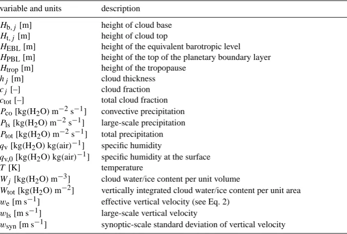
Table 1. List of symbols used throughout the paper. Long dash in the first column indicates that the corresponding variable is

non-dimensional. Variable modifiers:jindicates cloud type (=sl,sm,sh,co), andkstands for cloud phase (=drop,ice).

variable and units description

Hb,j[m] height of cloud base

Ht,j[m] height of cloud top

HEBL[m] height of the equivalent barotropic level HPBL[m] height of the top of the planetary boundary layer

Htrop[m] height of the tropopause

hj [m] cloud thickness

cj[–] cloud fraction

ctot[–] total cloud fraction

Pco[kg(H2O)m−2s−1] convective precipitation Pls[kg(H2O)m−2s−1] large-scale precipitation Ptot[kg(H2O)m−2s−1] total precipitation qv[kg(H2O)kg(air)−1] specific humidity

qv,0[kg(H2O)kg(air)−1] specific humidity at the surface

T [K] temperature

Wj[kg(H2O)m−3] cloud water/ice content per unit volume

Wtot[kg(H2O)m−2] vertically integrated cloud water/ice content per unit area we[m s−1] effective vertical velocity (see Eq. 2)

wls[m s−1] large-scale vertical velocity

wsyn[m s−1] synoptic-scale standard deviation of vertical velocity

in cloud albedo and lifetime respectively; both effects results from an impact of hydroscopic aerosols on the size of clouds droplets and ice crystals, e.g. Charlson et al., 1992; Solomon et al., 2007).

Among EMICs which currently have an effective single-layer cloudiness scheme are the models developed at the Potsdam Institute for Climate Impacts Research (Climber-2, Petoukhov et al., 2000; Ganopolski et al., 2001, and Climber-3α, Montoya et al., 2005) and at the A. M. Obukhov Insti-tute of Atmospheric Physics, Russian Academy of Sciences IAP RAS CM; see Mokhov and Eliseev (2012). Currently, both institutes are developing new versions of the EMICs (Coumou et al., 2011; Eliseev et al., 2011). As a part of this programme, we are working out a new cloud–precipitation scheme. This scheme describes three-layer stratiform clouds and one effective type of convection clouds.

In the present paper, the current version of the scheme is described and tested offline for the present-day climate.

2 Governing equations

The developed scheme considers four cloud types within a given grid cell. The first three cloud types describe low-level, mid-low-level, and upper-level stratiform clouds (thereafter denoted with the subscripts sl, sm, and sh respectively). This distinction corresponds to observational experience at large horizontal scales (Tian and Curry, 1989; Mazin and Khrgian, 1989). The fourth cloud type is denoted by subscript co and represents convective (cumulus) clouds.

The scheme is designed for use in Earth system models of intermediate complexity. This is the reason why we tried to keep all equations as simple as possible. The latter pre-cludes usage of more elaborated approaches which are imple-mented in the state-of-the-art global circulation models. In the present scheme, some equations are just derived heuristi-cally and tuned to observations (see below).

Values of basic variables are listed in Table 1. 2.1 Cloud vertical boundaries and extent

Height of convective clouds baseHb,cois related to the plan-etary boundary layer heightHPBL:

Hb,co=CH,coHPBL, (1)

whereCH,cois a constant. In addition, effective vertical ve-locity

we=wls+awe,1wsyn+awe,2woro+awe,3wconv (2)

(3)

here∇_His a horizontal gradient operator, andu(0)is near-surface horizontal wind). Effective vertical velocity in Eq. (2) is calculated similar to Eq. (36) in Petoukhov et al. (2000), but with coefficients awe,1 and awe,2 depending on cloud

type. An additional modification with respect to Eq. (36) in Petoukhov et al. (2000) is due to convective stirring: the term awE,5wconvis introduced with

wconv=wconv,0exp _q

v(0) qv,0

. (3)

Here qv(0) is near-surface specific humidity, wconv,0= 0.01 m s−1, and qv,0=0.01 kg(H2O)kg(air)−1. In the scheme,awE,3is set to zero for stratiform clouds. Thus, the

last term in Eq. (2) is applied only to convective clouds. It should be noted thatHb,comay depend on atmospheric moisture content as well. However, this dependence is rather weak (Mazin and Khrgian, 1989, p. 173, Eq. 1) and simply ignored in our work.

In the current setup, heights of stratiform cloud bases are related either to the height of the planetary boundary layer HPBLor to the height of the equivalent barotropic levelHEBL (which is defined as a level at which motions are equivalent to the vertical average of motions in the corresponding column; this level is close to the 500 hPa isobaric level (Holton, 2004, p. 450)) or to the height of the tropopauseHtrop(Petoukhov et al., 1998, 2003). AllHPBL,HEBL, andHtrop are external parameters of the scheme. The relations read

Hb,sl=CH,sl·HPBL,

Hb,sm=CH,sm·HEBL, (4)

Hb,sh=CH,sh·Htrop,

whereCH,sl,CH,sm, andCH,share parameters. This roughly corresponds to the observational evidence summarised in pp. 162–175 of the book by Mazin and Khrgian (1989). In particular, low-level stratiform cloud bases are typically located close to HPBL. Mid-level cloud bases are located, as a whole, slightly below equivalent barotropic level; their heights only weakly depend on season. Bases of the upper-level stratiform clouds are shallower in the higher latitudes than in the lower latitudes; the same is true for the tropopause height (Hoinka, 1998).

Calculation of geometric thickness of stratiform clouds is similar to that used in Petoukhov et al. (2000):

hj=hj,0·c_jlh·Fh,T ,j, (5)

wherecj is cloud fraction,j∈ {sl,sm,sh}stands for cloud type, parameterhj,0depends on this type,lhis constant, and the dependence on temperature is

Fh,T ,j=exp −Ch

Tj−Th,0

. (6)

HereChandTh,0are constants. Cloud temperatureTj is as-signed to the respective value at cloud base:

Tj=T Hb,j

.

Finally, heights of the stratiform cloud tops are computed according toHt,j=Hb,j+hj. Heights of convective cloud tops are related to the height of the tropopause

Ht,co=Ct,coHtrop. (7)

Geometric thickness of convective clouds is calculated as Ht,co−Hb,co. In Eq. (7),Ct,cois a function of specific hu-midity (via vertical velocity due to convective stirringwconv, see Eq. 3):

Ct,co=Ct,co,1+Ct,co,2· wconv wconv,0

, (8)

with an additional constraint that Ct,co is smaller than the prescribed valueCt,co,max. In Eq. (8),Ct,co,1andCt,co,2are constants.

Thus calculated heights are associated with the nearest vertical level corresponding to input variables.

2.2 Cloud fraction

For stratiform clouds, cloud fractions (i.e. the fraction of the area covered by clouds of typej) are calculated similar to Eq. (35) in Petoukhov et al. (2000):

cj=RH(Hb,j)lRH,jFc,we,j. (9)

Here RH(Hb,j)is relative humidity at cloud bases,lRH,jis a constant, and

Fc,we,j=Cc,1,j+

1

2Cc,2,j 1+tanh

we Hb,j

we,0 !

. (10)

In Eq. (10),Cc,1,j,Cc,2,j, andwe,0are constants. Similar to other diagnostic cloud schemes used in global climate mod-els, our scheme assumes positive correlation between relative humidity and cloud fraction. In turn,Fc,we,j represents the

impact of synoptic-scale, convective, and orographic stirring on cloud formation. Basically, this stirring enhances cloud fraction, but saturates at highwe.

Convective clouds are allowed to develop only ifweis pos-itive. If this condition is fulfilled, convective cloud fraction is computed according to Eq. (38) in Petoukhov et al. (2000):

cco=cco,0tanh

we Hb,co

we,co

tanhqv(0) qv,co

. (11)

Here cco,0, we,co, and qv,co are constants. Similar to Eqs. (9) and (10), Eq. (11) was derived heuristically assum-ing that cco should increase if either atmospheric moisture content or synoptic-scale, convective, and orographic stir-ring is increased. Again, both dependences should saturate at largeqv(0)andwerespectively.

(4)

If this condition is not met, convective cloud fraction is re-duced tocco=1−cj. In other words, if both stratiform and convective clouds coexist in a given grid cell, the former is considered to be favoured.

Total cloud fractions are computed by overlapping clouds at different levels. Convective clouds are always considered as a single column with maximum overlap between individ-ual computational layers. For stratiform clouds, a random overlap between low-, mid-, and upper-level clouds is al-ways used. However, if, for example,Ht,co> Hb,sm, then the area covered by cumulus clouds is removed from the latter random overlap for low- and mid-level stratiform clouds. A similar approach, but extended to the upper-level stratiform clouds as well, is used ifHt,co> Hb,sh.

2.3 Cloud water and ice content

For stratiform clouds, the cloud water path (commonly de-fined as the column amount of liquid and frozen water in clouds) is calculated after Eq. (2) on p. 332 in Mazin and Khrgian (1989):

Wj=αWhjFW,j, (12)

where FW,j =exp

rMK Tj−Tf/Tj, (13)

Tf=273.16 K, andαW andrMKare constants; here the sub-script “MK” indicates that this equation is adapted from Mazin and Khrgian (1989). Cloud water content is then dis-tributed vertically, assuming that lateral boundaries of strat-iform clouds are vertical and Wj profile is homogeneous within the cloud.

For convective clouds, total cloud water pathWco is cal-culated by integrating the respective vertical profile over the cloud depth

Wco= Ht,co

Z

Hb,co

Qco(z)dz. (14)

HereQco(z)is volumetric cloud water/ice content which is computed using Eq. (1) on p. 337 in Mazin and Khrgian (1989):

Qco(z)=Qco,max× _ζ

ζ0

mMK₁₋_ζ 1−ζ0

nMK

, (15)

where

ζ= z−Hb,co

/ Ht,co−Hb,co

,

mMK=2.8, nMK=0.57,

ζ0=mMK/ (mMK+nMK) .

In turn, maximum volumetric water/ice content in convec-tive clouds, Qco,max is approximated based on the results reported in Fig. 2 on the same page in Mazin and Khrgian (1989):

Qco,max=b1,MK Ht,co−Hb,co+

b2,MK(Tco−273.16)−b3,MK, (16) whereb1,MK, b2,MK, and b3,MK are constants. In applying Eq. (16), an additional check thatQco,max≥0 is performed. For all cloud types, ice and droplet clouds are distin-guished. The molar fraction of frozen and non-frozen water molecules,ficeandfdrop respectively, at a given heightzis calculated according to Rotstayn (1997):

fice(z)=   

 

1 ,ifT (z) < Tm,1 Tm,2−T (z)

Tm,2−Tm,1 ,ifTm,1≤T (z)≤Tm,2,

0 ,ifT (z) > Tm,2,

(17)

fdrop(z)=1−fice(z).

The values ofTm,1andTm,2are assumed to be independent of cloud type.

Total cloud water path (per grid cell)Wtotis calculated as a weighted mean of Wj (j =sl,sm,sh,co) assuming the same overlap as for total cloud fraction.

2.4 Precipitation

Precipitation rate is computed as a sum of large-scale (strati-form) and convective precipitation:

Ptot=Pls+Pco. (18)

Large-scale precipitation is calculated by summing the contributions from all stratiform clouds in a given grid cell: Pls=Pls,sl+Pls,sm+Pls,sh,

with

Pls,j=cj· fdropPls,j,drop+ficePls,j,ice. (19) In turn,

Pls,j,k= Qj

τj,k ,

wherejindicates cloud type,kstands for cloud phase (either droplet or ice),Qjis volumetric water content in clouds, and τj,kis the lifetime of cloud typej in phasek.

Convective precipitation is attributed to cumulus clouds. It is calculated by integrating precipitation in the vertical direc-tion

Pco=cco· Ht,co

Z

Hb,co

(5)

wherepco represents the contribution to Pco from the in-finitesimally thin vertical layer. The latter is

pco=fdrop(z)pco,drop+fice(z)pco,ice, (21) and t he contribution from convective clouds in phasekreads pco,k=Qco/τco,k.

For all cloud types, lifetime is calculated similar to that in Petoukhov et al. (2000)

τj,k=τ0,j,k 1−aτFc,we,j

, (22)

where j ∈ {sl,sm,sh,co}, k∈ {drop,ice}, Fc,we,j is the

same as in Eq. (10), andaτ is a constant. We assume that lifetimes for liquid and frozen parts of clouds of all types in a given grid cell are linearly related to each other:

τj,ice=kτ,ice·τj,drop, (23)

wherekτ,ice is a constant. For liquid stratiform clouds (j ∈

{sl,sm,sh,}we assume that lifetime is a weak function of cloud fraction

τj,drop=τ0·c1_j/2 (24)

with the constantτ0. Thus, clouds which are more horizon-tally extensive exist longer than smaller (presumably broken) clouds. A similar assumption for convective clouds is not needed because these clouds basically exists as systems of localised towers. Therefore, for liquid convective clouds,

τco,drop=τ0/ kτ,conv, (25)

andkτ,convis a constant.

Note that the partition between ice and liquid cloud parti-cles may be changed during their fall to the ground. As a re-sult, it is impractical to useficeorfdropto calculate rain- or snowfall rate at the surface. It is assumed to be calculated by the model’s land surface scheme based on surface tempera-ture.

3 Calibration

3.1 An approach

First of all, the scheme was tuned manually to arrive at the parameter values listed in Table 2. This was done in order to set a reasonable starting point for the automated calibration procedure described below. This parameter set as well as the simulations with this set are referred to as initial.

In the latter automated calibration, governing parameters of the scheme were sampled by using the Latin hypercube sampling (McKay et al., 1979; Stein, 1987). We chose only to sample the parameters which are either most uncertain or those which modify the results of calculations with the

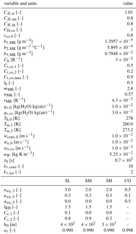
Table 2. List of the standard values of the governing parameters of

the scheme. Long dash in the first column indicates that the cor-responding variable is non-dimensional, and in the last column it shows that a specific parameter is not applied to cumulus clouds.

variable and units value

C_H,_sl[–] 1.01

CH,sm[–] 0.8

C_H,_sh[–] 0.8

CH,co[–] 1

c_co_,₀[–] 0.8

b₁_,_MK[g m−4] 1.2957×10−5

b2,MK[g m−3◦C−1] 5.895×10−4

b₃_,_MK[g m−3] 0.7848×10−2

Ch[K−1] 3×10−2

C_t_,_co_,₁[–] 0.5

Ct,co,2[–] 0.2

Ct,co,max[–] 0.9

l_h[–] 0.5

mMK[–] 2.8

n_MK[–] 0.57

rMK[K−1] 4.3×10−2

q_v_,₀[kg(H2O)kg(air)−1] 1.0×10−2

qv,co[kg(H2O)kg(air)−1] 3.0×10−2

T_h_,₀[K] 278

Tm,1[K] 260.0

T_m_,₂[K] 273.2

w_conv_,₀[m s−1] 1.0×10−2

we,0[m s−1] 1.0×10−2

we,co[m s−1] 1.0×10−3

αW[kg K m−3] 5.25×10−2

τ₀[s] 0.7×103

kτ,conv[–] 10

k_τ,_ice[–] 2

SL SM SH CO

a_w_E_,₃[–] 5.0 2.0 2.0 0.5

a_w_E_,₄[–] 0.3 0.3 0.3 0.1

a_w_E_,5[–] 0.0 0.0 0.0 0.5

l_RH[–] 1.5 1.5 1.5 –

Cc,1[–] 0.1 0.0 0.0 –

C_c_,₂[–] 0.8 0.9 0.3 –

h0[m] 4×102 4×102 3×103 –

aτ[–] 0.990 0.990 0.990 0.998

scheme most strongly. In addition, some parameters are re-dundant in the scheme (e.g. any change ofwconv,0 may be compensated by an opposite relative change in the value of awE,3), and for some it is unclear how to prescribe their prior

(6)

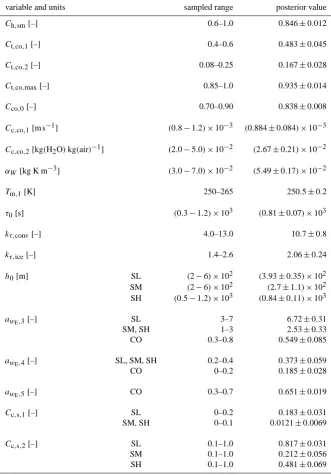
Table 3. List of the perturbed parameters of the scheme together with their priory ranges. Long dash in the first column indicates that

the corresponding variable is non-dimensional. The symbols “SL”, “SM”, “SH”, and “CO” indicate particular cloud types according to classification used in the scheme. In the last column, Bayesian mean and standard deviation are shown.

variable and units sampled range posterior value

C_h,sm[–] 0.6–1.0 0.846±0.012

C_t,co,1[–] 0.4–0.6 0.483±0.045

C_t,co,2[–] 0.08–0.25 0.167±0.028

Ct,co,max[–] 0.85–1.0 0.935±0.014

C_co,0[–] 0.70–0.90 0.838±0.008

C_c,co,1[m s−1] (0.8−1.2)×10−3 (0.884±0.084)×10−3

C_c,co,2[kg(H₂O)kg(air)−1] (2.0−5.0)×10−2 (2.67±0.21)×10−2

αW [kg K m−3] (3.0−7.0)×10−2 (5.49±0.17)×10−2

T_m,1[K] 250–265 250.5±0.2

τ₀[s] (0.3−1.2)×103 (0.81±0.07)×103

k_τ,conv[–] 4.0–13.0 10.7±0.8

kτ,ice[–] 1.4–2.6 2.06±0.24

h₀[m] SL (2−6)×102 (3.93±0.35)×102

SM (2−6)×102 (2.7±1.1)×102 SH (0.5−1.2)×103 (0.84±0.11)×103

awE,3[–] SL 3–7 6.72±0.31

SM, SH 1–3 2.53±0.33

CO 0.3–0.8 0.549±0.085

awE,4[–] SL, SM, SH 0.2–0.4 0.373±0.059

CO 0–0.2 0.185±0.028

awE,5[–] CO 0.3–0.7 0.651±0.019

C_c,s,1[–] SL 0–0.2 0.183±0.031

SM, SH 0–0.1 0.0121±0.0069

C_c,s,2[–] SL 0.1–1.0 0.817±0.031

SM 0.1–1.0 0.212±0.056

SH 0.1–1.0 0.481±0.069

ice contentWtot, and total precipitation ratePtot. In addition, to assess partition between stratiform and convective clouds, a contribution toPtotfrom large-scale and convective precip-itation is assessed as well.

Total score for the scheme is calculated by multiplying the individual skills for cloud fractionsSc, cloud water pathSW, and precipitationSP:

S=ScSWSP. (26)

The goal of the optimisation procedure is

S→max. (27)

Skill score for cloud fraction is constructed from its glob-ally and annuglob-ally averaged value, and fields for annual mean, January, and July cloud fractions:

(7)

A. V. Eliseev et al.: Scheme for cloudiness and precipitation for EMICs 1751

For globally and annually averaged cloud fraction Sc,g=N ctot,g,ann,M;ctot,g,ann,O, σctot,g,ann,O

, (29)

where isN(X;Xm, σX)is a normal distribution function of variableXwith meanXmand standard deviationσX. In turn, ctot,g,ann is the globally and annually averaged total cloud fraction. Here and below, indices M and O stand for mod-elled and observed fields, respectively. Skills Sc,ann, Sc,Jan, andSc,Julare computed as in Taylor (2001):

SX=TX, (30)

whereXstands for any of “c,ann”, “c,Jan”, and “c,Jul”, and function

TX =

(1+rX)4

(AX+1/AX)2

. (31)

In Eq. (31)rXis the coefficient of the spatial correlation between area-weighted modelled and observed fields ofX, andAX is the so-called relative spatial variation calculated according to

AX=AX,M/AX,O, (32)

where A2_X,_M is the spatial average of XM−XM,g 2

, and XM,g is a globally (but not necessarily annually) averaged value of the modelled fieldXM. In turn,AX,Ois defined sim-ilar toAX,Mbut for the observed field.

Skill score for cloud water content is calculated by using an equation similar to Eq. (28):

SW=SW,gSW,annSW,JanSW,Jul. (33) The meaning of terms on the right-hand side of Eq. (33) is analogous to that in Eq. (28). This is only applied for total (vertically integrated) cloud water pathWtot. The procedure to calculate terms on the right-hand side of Eq. (33) is again similar to Eqs. (29) and (30).

Precipitation skill score is

SP=SP,gSP,annSP,JanSP,Jul. (34) Because it is important to distinguish between large-scale and convective precipitation,PlsandPco respectively, indi-vidual terms in Eq. (34) are calculated differently from their counterparts in Eqs. (28) and (33). In particular,

SP,g=SP,tot,gSP,rat,g, (35) where

SP,tot,g=N Ptot,g,ann,M;Ptot,g,ann,O, σPtot,g,ann,O

,

SP,rat,g=N prat,g,ann,M;prat,g,ann,O, σprat,g,ann,O

. (36)

a) NH

Jan Feb Mar Apr May Jun Jul Aug Sep Oct Nov Dec 0.52

0.54 0.56 0.58 0.6 0.62 0.64 0.66 0.68 0.7

ctot

b) SH

Jan Feb Mar Apr May Jun Jul Aug Sep Oct Nov Dec 0.5

0.55 0.6 0.65 0.7 0.75

ctot

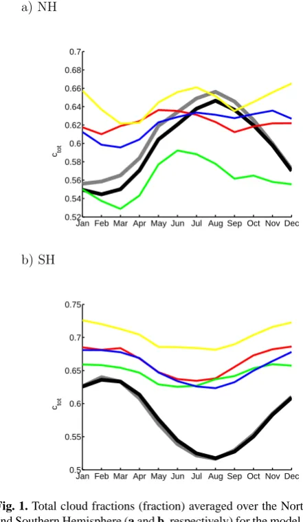
Figure 1:

1

Fig. 1.Total cloud fractions (fraction) averaged over the Northern and Southern Hemispheres (aandbrespectively) for the model with initial guess and calibrated parameter sets (gray and black lines correspondingly) as well as for the ISCCP, MODIS, CERES, and ERA-40 data sets (red, yellow, green, and blue curves correspondingly).

Fig. 1. Total cloud fractions (fraction) averaged over the Northern

and Southern Hemisphere (a and b, respectively) for the model with initial guess and calibrated parameter sets (grey and black lines re-spectively) as well as for the ISCCP, MODIS, CERES, and ERA-40 data sets (red, yellow, green, and blue curves respectively).

HerePtot=Pls+Pco,prat=Pco/Pls. Further,

SP,ann=SP,tot,annSp,rat,ann. (37) Here

SP,tot,ann=TP,tot,ann, (38)

Sp,rat,ann=Tp,rat,ann. (39)

The termsSP,Jan andSP,Jul are calculated by using equa-tions similar to Eqs. (37)–(39) but with respective monthly mean fields in place of annual mean ones.

(8)

16 A. V. Eliseev et al.: Scheme for cloudiness and precipitation for EMICs

a) initial

b) calibrated

c) ISCCP D2

d) CERES

e) MODIS

f) ERA–40

Figure 2:

2

Fig. 2.Annual mean modelled total cloud fraction (fractions) for initial and calibrated parameter sets (aandbcorrespondingly) in comparison

to the ISCCP D2, CERES, MODIS, and ERA-40 climatologies (c,d,e, andfrespectively).

Fig. 2. Annual mean modelled total cloud fraction (fractions) for initial and calibrated parameter sets (a and b, respectively) in comparison

to the ISCCP D2, CERES, MODIS, and ERA-40 climatologies (c, d, e, and f, respectively).

We checked different procedures to obtain this optimal pa-rameter set. In particular, we have tried to zero weights if S’s were smaller than the half of their maximum. In this ap-proach, ensemble mean values were basically unchanged but their standard deviations were smaller. In addition, we have tried to manually select a best-performing sample and use its parameters as optimal. However, in the latter approach no pa-rameter sample was superior with respect to their Bayesian means.

3.2 Forcing data and observational data sets

(9)

used. The lowermost level was located at the Earth’s surface, and the next one was at HPBL. Other levels were equally spaced in height up to the tropopause. The latter was diag-nosed from the monthly mean ERA-40 data using the con-ventional definition for thermal tropopause.

For total cloud fractions, the following monthly climatolo-gies were used:

– The International Satellite Cloud Climatology Project (ISCCP) product D2 (Rossow and Duenas, 2004). IS-CCP based on 3-hourly radiance data from visible (0.8 µm) and infrared (11 µm) channels measurements with the horizontal resolution 4–7 km from weather geostationary satellites (GEO) (like GMS, GOES East, GOES West, Meteosat, MTSAT, INSAT; see Rossow and Duenas (2004) for more details) and National Oceanic and Atmospheric Administration (NOAA) polar-orbiting (low Earth orbit, LEO) satellites. Data are intercalibrated between GEO and LEO satellites. Cloud fraction is derived by using the spectral thresh-old test and a combination of the spatial and temporal uniformity tests.

– The Clouds and the Earth’s Radiant Energy System (CERES) (Minnis et al., 2011). This data set was created by simultaneous retrievals of cloud proper-ties and broadband radiative fluxes from the instru-ments on two LEO Terra and Aqua satellites from the Earth Observing System. The data from the Terra satellite with 10:30/22:30 LT equatorial crossing were used. Cloud properties are determined using measure-ments by the Moderate Resolution Imaging Spectro-radiometer (MODIS; see below). MODIS provides measurements in 36 spectral channels with resolution from 0.25 to 1 km. Five of them (with the central wave-lengths of 0.65, 1.64, 3.75, 11, and 12 µm) are used in the CERES cloud mask.

– The MODIS Science Team (MODIS-ST) data set (Frey et al., 2008). Instead of the CERES algorithm, 14 of 36 spectral channels of MODIS instruments (with the central wavelengths from 0.66 to 13.94 µm) are used in the MODIS-ST cloud mask algorithm to dis-criminate cloud pixels from clear sky.

– ERA-40 reanalysis data (Simmons and Gibson, 2000). This data set is affected by imperfections of the fore-cast model. This is especially true for cloud-related variables belonging to the so-called class “C”. How-ever, because our simulations will be forced by the ERA-40 data, it is instructive to compare simulation output with that reanalysis data.

Basically, satellite retrievals reliably detect total cloud frac-tion. However, because of the “satellite view” of cloud layers (upper cloud layers may mask lower ones) mid- and lower-level cloud fractions detection is not straightforward. This is

Table 4. Globally and annually averaged values as calculated by

the proposed scheme with two parameter sets in comparison with the available observational data.

variable initial calibrated observational data sets

0.62 (ISCCP)

0.59 0.59 0.67 (MODIS)

ctot[–] 0.60 (CERES)

0.64 (ERA-40)

Wtot[g(H2O)m−2] 66 82 125 (CERES)

Ptot[cm yr−1] 101 100 88 (GPCP)

113 (ERA-40)

Pls/Ptot[–] 0.48 0.45 0.53 (ERA-40)

the basic reason why only total cloud fractions were used for calibration, and not cloud fractions in different layers. Another reason is the above-mentioned (see Sect. 2) differ-ence between the definition of the cloud layers in the present scheme and that used in common cloud products. An exten-sive intercomparison between these data sets was reported by Chernokulsky and Mokhov (2010, 2012). We setσctot,g,ann,Oto

0.1, which is a typical value for interannual standard devia-tion of globally averaged total cloud fracdevia-tions as estimated by using the ISCCP data.

Cloud water pathWtotwas evaluated against the CERES retrievals (Minnis et al., 2011). In this data set, the cloud wa-ter path is computed as function of cloud optical depth and appropriate effective particle size. ForSW,g,σcW_tot,g,ann,O is set

ad hoc to 0.1×cWtot,g,ann,O.

Total precipitation is compared with the GPCP-2.2 data set (Global Precipitation Climatology Project, version 2.2, an update from Huffman et al., 2009). Lacking purely em-pirical data about the subdivision of total precipitation into large-scale and convective precipitation, we have calibrated the scheme by using theprat calculated based on ERA-40 data. Note that while global annual precipitation fractions differ by 29 % (Table 4), the spatial pattern of precipitation rate in ERA-40 is close to that in GPCP data. For the GPCP-2.2 data,σPtot,g,ann,O=1.5 mm mo

−1_and_σ

prat,g,ann,O=0.1.

We arbitrarily divided these data into training and compar-ison sets. The training set consists of ISCCP data for cloud fraction, CERES data for cloud water path, GPCP data for to-tal precipitation, and ERA-40 data for fraction of large-scale precipitation in a total one. All other data were used only for comparison.

(10)

A. V. Eliseev et al.: Scheme for cloudiness and precipitation for EMICs 17

a) initial

b) calibrated

c) ISCCP D2

d) CERES

e) MODIS

f) ERA–40

Figure 3:

3 Fig. 3.Similar to Fig. 2 but for January.Fig. 3. Similar to Fig. 2 but for January.

4 Results of calibration

Basically, the scheme with calibrated parameters agrees bet-ter with observations relative to its counbet-terpart with the ini-tial parameter set. This is evident even at the global scale, with most marked improvement for cloud water path Wtot (Table 4). Slight deterioration is visible for the fraction of convective precipitation in total precipitation.

4.1 Cloud fractions

At the global scale, cloud fractions simulated by the scheme with the calibrated parameter set equal 0.59, which is slightly below the observational range 0.60–0.67 (Table 4); more

extensive comparison of different empirical data sets leads to the value 0.66 ± 0.02 (Chernokulsky and Mokhov, 2010). The simulated value for the scheme with the calibrated pa-rameters set is very close to that for the version with the ini-tial set of parameters.

(11)

a) initial

b) calibrated

c) ISCCP D2

d) CERES

e) MODIS

f) ERA–40

Figure 4:

4 Fig. 4.Similar to Fig. 2 but for July._{Fig. 4. Similar to Fig. 2 but for July.}

fraction during the cold (warm) part of the year. However, the amplitude of the annual cycle for modelledctotis greater than the satellite-derived one, especially in the Southern Hemi-sphere.

The scheme broadly reproduces the geographical pattern of cloud fractions. Similar to observations, annual mean total cloud fraction, ctot, attains maxima in northern and south-ern mid-latitudes, wherectotis typically between 0.7 and 0.9 (Fig. 2a and b). This is in general agreement with empiri-cally derived values over oceans (Fig. 2c–f). However, over land our scheme with the initial parameter set overestimates total cloud fraction in this latitudes, since satellite-based data show smaller cloud fractions (from 0.5 to 0.7 from ISCCP

and MODIS, and even from 0.3 to 0.7 from CERES). This bias is slightly diminished upon calibration. This is accom-panied by reduced total cloud fraction over mid-latitudinal oceans, which worsens the agreement with observations. In the subtropics, the simulated total cloud fractions range from 0.1 to 0.5, which is too small in comparison to observations. Note that too-deep subtropical minima ofctotbecome shal-lower upon calibration. The fraction of convective clouds over the Indo-Pacific warm pool and over the Amazon Basin in our scheme (0.7 and larger) generally agrees with obser-vations.

(12)

a) initial, low–level

b) calibrated, low–level

c) initial, mid–level

d) calibrated, mid–level

e) initial, upper–level

f) calibrated, upper–level

Figure 5:

5

Fig. 5. Annual mean low-level cloud fractioncl≡csl+cco(aandb), mid-level cloud fractioncm≡csm(candd), and upper-level cloud

fractionch≡csh(eandf) for the model versions with initial (a,cande) and calibrated (b,dandf) parameter sets. The units are fractions.

Fig. 5. Annual mean low-level cloud fractioncl≡csl+cco(a and b), mid-level cloud fractioncm≡csm(c and d), and upper-level cloud fractionch≡csh(e and f) for the model versions with initial (a, c and e) and calibrated (b, d and f) parameter sets. The units are fractions.

fields for individual months (Figs. 3 and 4). For all months, the scheme realistically reproduces total cloud fractions over mid-latitudinal oceans, but overestimatesctotover land at the same latitudes. That overestimate is more marked in winter than in summer, which is consistent with the overestimated amplitude of the annual cycle ofctot. Subtropical minima are too deep throughout the year. However, the scheme correctly places abundant convective clouds near the Equator in the winter hemisphere.

Comparison of the simulated cloud fractions in different layers with observations is not straightforward. The first rea-son for that is due to differences in the classification of

(13)

a) NH

Jan Feb Mar Apr May Jun Jul Aug Sep Oct Nov Dec 50 60 70 80 90 100 110 120 130 140 W tot , g(H 2 O)m −2 b) SH

Jan Feb Mar Apr May Jun Jul Aug Sep Oct Nov Dec 40 60 80 100 120 140 160 180 W tot , g(H 2 O)m −2 Figure 6: 6

Fig. 6.Cloud water path (g(H2O)m−2) averaged over the Northern and Southern Hemispheres (aandbrespectively) for the model with initial and calibrated parameter sets (gray and black lines correspondingly) as well as for the CERES data set (green).

Fig. 6. Cloud water path (g(H2O)m−2) averaged over the Northern and Southern Hemisphere (a and b respectively) for the model with initial and calibrated parameter sets (grey and black lines respec-tively) as well as for the CERES data set (green).

view” of cloud layers in common cloud satellite products (see Sect. 3.2).

However, some comparison may be performed with the re-sults reported by Mace et al. (2009), who used the same clas-sification scheme as we do for the merged lidar and radar ob-servations from CALIPSO and CloudSat satellites. For this comparison, however, we have to keep in mind that Mace et al. (2009) reported only one year of measurements (from July 2006 to June 2007), which is quite different from the long-term climatology which we attempt to simulate here. For the reader’s convenience, Fig. 5 is redrawn in the Supple-ment of the present paper (Fig. S1) in a fashion compatible with relevant figures from Mace et al. (2009). In turn, the lat-ter figures are reproduced in Fig. S2 of the Supplement with permission of Wiley and Sons Inc.

In particular, our annual mean low-level cloud fraction cl=csl+ccomay be compared to their Fig. 10a. Our scheme with the initial parameter set simulatesclbetween 0.6 and 0.7 over the mid-latitudes and in the areas of tropical convection, and from 0.1 to 0.5 in the subtropics (Fig. 5a). The largestcl (above 0.7) is simulated over the Antarctic. Upon calibra-tion, cl in the northern and southern mid-latitudes is from 0.4 to 0.6, and over the Antarctic it is increased to values of 0.8 and larger. (Fig. 5b). In the middle latitudes, the cali-bration improves the agreement with the retrievals by Mace et al. (2009). In the subtropics, cl is somewhat increased, which again improves the agreement. Maxima ofclover the Indo-Pacific warm pool and over Amazonia become broader, which deteriorates our simulations.

One limitation of the present scheme is the lack of stra-tocumulus (Sc) decks over the eastern parts of the oceans. Annual mean stratocumulus cloud fraction in these regions fractions may be as large as 0.6 (Wood, 2012), and yields about 80–90 % of all low-level cloud fraction here. Our scheme produces low-level cloud fractions in these regions smaller than 0.2, which underestimate markedly the observed one. It is likely that this underestimate is due to neglect-ing the impact of atmospheric inversions on cloud forma-tion. Such inversions suppress moisture fluxes from the plan-etary boundary layer to the free troposphere. In turn, un-der these conditions, vertical profile of specific (and relative) humidity may deviate strongly from the respective monthly averaged profile. An implementation of this impact may be one future improvement for our scheme. Note, however, that ERA-40 data underestimate the satellite-derived cloud frac-tion in these regions as well. This is an example of a problem that most contemporary cloudiness schemes in global climate models (GCMs) have in representing stratocumulus decks. In particular, Lauer and Hamilton (2013) reported that the lat-est generation of these models, the CMIP5 (Coupled models Intercomparison Project, phase 5) GCMs, underestimate the amount of subtropical stratocumulus decks by 30–50 %.

Mid-level cloud fractionscm≡csmmay be compared with Fig. 11 from Mace et al. (2009). In the version with the ini-tial parameter set, mid-level cloud fractions range from 0.3 to 0.5 in mid-latitudes and the convective regions in the trop-ics (Fig. 5c). In other tropical and subtropical regions,cmis below 0.2 everywhere. Upon calibration, everywhere in the tropics and subtropicscm<0.1, and in higher latitudescm is between 0.1 and 0.2 (Fig. 5d). This drastically improves agreement with the hydrometeor fractions with bases from 3 to 6 km reported in Fig. 11 of Mace et al. (2009).

(14)

a) initial

b) calibrated

c) CERES

Figure 7:

7

Fig. 7.Annual mean modelled total cloud water path (g(H2O)m−2) for initial and calibrated parameter sets (aandbcorrespondingly) in comparison to the CERES climatologyFig. 7. Annual mean modelled total cloud water path ( g(c). (H2O)m

−2_{) for initial and calibrated parameter sets (a and b, respectively) in} comparison to the CERES climatology (c).

a) initial

b) calibrated

c) CERES

Figure 8:

Fig. 8._{Fig. 8. Similar to Fig. 7 but for January.}Similar to Fig. 7 but for January.

(15)

a) initial

b) calibrated

c) CERES

Figure 9:

9

Fig. 9.Similar to Fig. 7 but for July. Fig. 9. Similar to Fig. 7 but for July.

the scheme’s performance. In particular, extratropical upper-level cloud fractions become broadly realistic, while there is an underestimation ofchin the areas of tropical convection by a factor of 2.

4.2 Cloud water path

Cloud water path (per model grid cell)Wtotis markedly in-creased during calibration. In the initial version, globally and annually averaged Wtot is equal to 66 g(H2O)m−2, which is about one-half the respective value derived from CERES, 125 g(H2O)m−2(Table 4). After calibration, modelledWtot increases to 82 g(H2O)m−2, which is again too small in comparison to observations, but the agreement is better. However, we note thatWtotin the CERES data is uncertain by a factor of 2. Further, the state-of-the-art general circulation models exhibit quite diverse simulation of this variable as well. In particular, the present-day globally averaged ensem-ble meanWtotfor CMIP5 GCMs is 87 g(H2O)m−2 (which is close to our value), and the respective intermodel range is 37–167 g(H2O)m−2(Lauer and Hamilton, 2013).

The modelled cloud water path averaged over the Northern and Southern Hemisphere show maxima in summer (Fig. 6). Calibration slightly decreases Wtot in the extratropics throughout the year and markedly increases it in the tropics. Annual mean cloud water path in both versions of the scheme is from 20 to 80 g(H2O)m−2(Fig. 7a). Over land it broadly agrees with the CERES data, while the cloud water path is

too small over the storm-track-affected regions. Over oceans, it is a strong underestimate (Fig. 7c). In the tropics, calibra-tion increases annual meanWtotby 20–50 %. As a result, the calibrated values ofWtot in the tropics agree slightly better with the CERES data than the initial ones. In addition,Wtot is too small in comparison to the CERES data. However, in these regions the CERES data suffer from large uncertainty (Minnis et al., 2011).

In winter, the cloud water path is severely underestimated, especially over land (Figs. 8 and 9). While one has to bear in mind that there is large uncertainty in the CERES retrievals in the high latitudes, an underestimate is clear in the middle latitudes. In summer, the mid-latitudinal cloud water path is somewhat small in comparison to the CERES data, but is rea-sonable as a whole. In contrast, in the tropics,Wtotis some-what too high, but the latter bias is markedly smaller than that in the middle latitudes in winter.

The largest contribution to Wtot comes from low-level stratiform clouds during all seasons, and from mid-level stratiform clouds during the warm part of the year (not shown). In the tropics, the contribution from convective clouds is also valuable.

(16)

stratiform clouds is likely too small in our model. In particu-lar, the typical thickness of low-level stratiform cloudshslin middle latitudes is from 150 to 300 m. The latter is markedly smaller than (very limited) observational data summarised by Mazin and Khrgian (1989, p. 188), for whichhsl≥300 m. We note that low-level stratiform clouds are major contribu-tors toWtotin the middle latitudes. This is similar for upper-level stratiform clouds: in our calculations,hshin middle lat-itudes is slightly larger than 100 m, while according to ob-servations these clouds could be as thick as 1 km (Mazin and Khrgian, 1989, p. 189). Thus, the scheme might be improved by revising Eq. (5). Additional source of error inWtotis due to underestimated cloud fraction in the storm tracks (recall that ourWtotis per grid cell rather than per cloudy part of the cell). Finally, the current version of the scheme completely lacks cloud–aerosol interaction, which increases clouds’ life-times and therefore enhances their water content (Twomey, 1974; Albrecht, 1989; Hobbs, 1993; Lohmann and Feichter, 2005).

General underestimation of cloud water path in the trop-ics is common for the contemporary global climate models as well, e.g. for the CMIP5 GCMs (Jiang et al., 2012; Lauer and Hamilton, 2013). In the storm tracks, the same models display a diverse behaviour, with some models underestimat-ingWtot, and others overestimating it. As a result, biases in our simulations are within the characteristic range of contem-porary climate models.

4.3 Precipitation

Annual global precipitation changes insignificantly during calibration. In the version with the initial parameter set it is equal to 101 cm yr−1, and in the calibrated version it is 100 cm yr−1. Both values are within the range set by the GPCP data (88 cm yr−1) and by the ERA-40 (113 cm yr−1) (Table 4). The fraction of large-scale precipitation in the ini-tial version is 0.48, which is an underestimate relative to the ERA-40 data (0.53). It becomes even smaller (0.45) after cal-ibration (Table 4).

For monthly precipitation averaged over the Northern and Southern Hemisphere, both initial and calibrated versions reasonably agree with empirical climatologies (Fig. 10). The calibration enhances precipitation in the storm tracks, and suppresses it elsewhere. In the calibrated version, monthly precipitation in the Northern (Southern) Hemisphere changes from 7 cm mo−1 (6 cm mo−1) in winter to 11 cm mo−1 (14 cm mo−1) in summer.

Upon calibration, annual precipitation slightly decreases in the middle latitudes and in the monsoon-affected region and markedly increases in the tropics (Fig. 11a and b). In the calibrated version, precipitationPtot ranges from 90 to 180 cm yr−1 in the middle latitudes. This is a decrease by about one-fourth from the initial version. In turn, in the moist tropics, the calibrated precipitation ranges from 180 to 300 cm yr−1, which is a respective increase by a factor 1.5. In

a) NH

Jan Feb Mar Apr May Jun Jul Aug Sep Oct Nov Dec 6 7 8 9 10 11 12 13 Ptot

, cm mo

−1

1 1.2 1.4 1.6 1.8 2 6 6.2 6.4 6.6 6.8 7 7.2 7.4 7.6 7.8 8 initial calibrated GPCP ERA−40 b) SH

Jan Feb Mar Apr May Jun Jul Aug Sep Oct Nov Dec 5 6 7 8 9 10 11 12 Ptot

, cm mo

−1

Fig. 10. Total precipitation (cm mo−1) averaged over the Northern and Southern Hemisphere (a and b respectively) for the model with standard and calibrated parameter sets (grey and black lines respec-tively) as well as for the GPCP and ERA-40 data sets (magenta and blue curves respectively).

dry subtropics, precipitation does not change markedly dur-ing calibration, bedur-ing below 60 cm yr−1. In most regions, the calibrated annual precipitation values agree better with the GPCP and ERA-40 climatologies than the initial ones.

(17)

a) initial

b) calibrated

c) GPCP

d) ERA–40

Figure 11:

11

Fig. 11.Annual modelled total precipitation (cmyr−1

) for initial and calibrated parameter sets (aandbcorrespondingly) in comparison to the GPCP and ERA-40 climatologies (candd).

Fig. 11. Annual modelled total precipitation (cm yr−1) for initial and calibrated parameter sets (a and b, respectively) in comparison to the GPCP and ERA-40 climatologies (c and d).

a) initial

b) calibrated

c) GPCP

d) ERA–40

Figure 12:

Fig. 12.Similar to Fig. 11 but for January total precipitation (cmmo−1 ).

Fig. 12. Similar to Fig. 11 but for January total precipitation (cm mo−1).

(18)

a) initial

b) calibrated

c) GPCP

d) ERA–40

Figure 13:

13

Fig. 13.Similar to Fig. 12 but for July. Fig. 13. Similar to Fig. 12 but for July.

It should be noted that the above-mentioned severe under-estimate of the fraction of stratocumulus decks in the sub-tropics should not severely affect simulation of precipita-tion because these clouds are non-precipitating ones (Houze, 1994). However, because our precipitation is somewhat too high in middle latitudes, and the cloud water path is too small there, it is likely that the calibrated lifetimes for stratiform clouds are too small, probably by a factor of 2.

5 Conclusions

This paper presents a scheme for calculation of the charac-teristics of multi-layer cloudiness and associated precipita-tion designed for climate models of intermediate complexity (EMICs). In contrast to the schemes previously used in such models, the scheme considers three-layer stratiform cloudi-ness and single-column convective clouds. It distinguishes between ice and droplet clouds as well. All main cloudiness characteristics (cloud fraction, cloud water path) are calcu-lated interactively. Precipitation is calcucalcu-lated by using cloud lifetime, which depends on cloud type and phase as well as on statistics of synoptic and convective disturbances.

A novel approach for tuning this scheme was used. This approach was based on sampling of major governing param-eters of the scheme. The corresponding cost function was constructed based on total cloud fraction, cloud water path, and precipitation, taking into account global mean values and

annual mean, January, and July spatial distributions for these variables. Bayesian averaging was used to calculate the opti-mal parameters set.

After calibration, the scheme realistically reproduces the main characteristics of cloudiness and precipitation. The simulated globally and annually averaged total cloud frac-tion is 0.59, and the simulated globally averaged annual pre-cipitation is 100 cm yr−1. Both values agree with empirically derived values.

The scheme agrees with observations for total cloud frac-tions over mid-latitudinal oceans, but overestimatesctotover land at the same latitudes. The latter overestimate is more marked in winter than in summer. Subtropical minima are too deep throughout the year. The scheme correctly places abundant convective clouds near the Equator in the winter hemisphere, while it underestimates upper-level cloud frac-tion in the regions with strong convecfrac-tion.

Cloud water path is severely underestimated by the scheme. In particular, major storm tracks contain too lit-tle water. Cloud water path of tropical convective clouds is reproduced reasonably. However, we note that satellite re-trievals for this variable are very uncertain, and the state-of-the-art general circulation models exhibit quite a diverse sim-ulation ofWtot.

(19)

still remain in the scheme, e.g. too little precipitation in the tropical area.

Note that our calibration is not a simple “fitting exercise”. In particular, cloud fractions at different layers were not trained explicitly during calibration. Nevertheless, they agree with available (rather limited) empirical data. This gives con-fidence in the physical basis of our scheme. Our scheme, while exhibiting some important biases, is a substantial im-provement for Earth system models of intermediate complex-ity.

However, regional and seasonal biases still present in the calibrated version show that there is a room for improvement of the scheme. One line of improvement may be the imple-mentation of stratiform clouds originating from convective anvils in the upper troposphere in the presence of strong winds (Mazin and Khrgian, 1989; Houze, 1994). This may ameliorate too small upper-level cloud fractions in the trop-ical convective regions in the current version of the scheme. Another major improvement should be an implementation of stratocumulus decks representation, which should improve cloudiness over the eastern parts of the oceans. This imple-mentation has to take into account inversion layers trapping convection and limiting vertical development of convective clouds (Wood, 2012). In addition, this version of the scheme lacks aerosol–cloud interaction (Twomey, 1974; Albrecht, 1989; Hobbs, 1993; Lohmann and Feichter, 2005). We note that one approach to include the latter in climate models of intermediate complexity has been developed by Bauer et al. (2008). An updated version of their scheme is planned to be implemented in our scheme in the future.

Supplementary material related to this article is available online at http://www.geosci-model-dev.net/6/ 1745/2013/gmd-6-1745-2013-supplement.pdf.

Acknowledgements. The authors thank the anonymous reviewers, whose comments greatly improved the paper. This work has been supported by the President of Russia grants 5467.2012.5 and 3259.2012.5, by the Russian Foundation for Basic Research, and by the programmes of the Russian Ministry for Science and Education (contract 14.740.11.1043 and agreement 8617), as well as by the Russian Academy of Sciences (programmes of the Presidium RAS, programmes by the Department of Earth Sciences RAS, and contract 74-OK/1-4).

Edited by: D. Roche

References

Albrecht, B.: Aerosols, cloud microphysics, and fractional cloudi-ness, Science, 245, 1227–1230, 1989.

Bauer, E., Petoukhov, V., Ganopolski, A., and Eliseev, A.: Climatic response to anthropogenic sulphate aerosols versus well-mixed greenhouse gases from 1850 to 2000 AD in CLIMBER-2, Tellus, 60B, 82–97, doi:10.1111/j.1600-0889.2007.00318.x, 2008. Bony, S., Colman, R., Kattsov, V., Allan, R., Bretherton, C.,

J.-L., D., Hall, A., Hallegatte, S., Holland, M., Ingram, W., Ran-dall, D., Soden, B., Tselioudis, G., and Webb, M.: How well do we understand and evaluate climate change feedback pro-cesses?, J. Climate, 19, 3445–3482, doi:10.1175/JCLI3819.1, 2006.

Cesana, G. and Chepfer, H.: How well do climate models simu-late cloud vertical structure? A comparison between CALIPSO-GOCCP satellite observations and CMIP5 models, Geophys. Res. Lett., 39, L20803, doi:10.1029/2012GL053153, 2012. Charlson, R., Schwartz, S., Hales, J., Cess, R.,

Coack-ley, J., Hansen, J., and Hofmann, D.: Climate forc-ing by anthropogenic aerosols, Science, 255, 423–430, doi:10.1126/science.255.5043.423, 1992.

Charney, J. and Eliassen, A.: A numerical method for predicting the perturbations of the middle latitude westerlies, Tellus, 1, 38–54, doi:10.1111/j.2153-3490.1949.tb01258.x, 1949.

Chernokulsky, A. and Mokhov, I.: Intercomparison of global and zonal cloudiness characteristics from different satellite and ground based data, Issledovaniye Zempli iz Kosmosa, 12–29, 2010 (in Russian).

Chernokulsky, A. and Mokhov, I.: Climatology of total cloudiness in the Arctic: an intercomparison of observations and reanalyses, Adv. Meteorol., 2012, 542093, doi:10.1155/2012/542093, 2012. Claussen, M., Mysak, L., Weaver, A., Crucifix, M., Fichefet, T., Loutre, M.-F., Weber, S., Alcamo, J., Alexeev, V., Berger, A., Calov, R., Ganopolski, A., Goosse, H., Lohmann, G., Lunkeit, F., Mokhov, I., Petoukhov, V., Stone, P., and Wang, Z.: Earth sys-tem models of intermediate complexity: closing the gap in the spectrum of climate system models, Clim. Dynam., 18, 579–586, doi:10.1007/s00382-001-0200-1, 2002.

Coumou, D., Petoukhov, V., and Eliseev, A. V.: Three-dimensional parameterizations of the synoptic scale kinetic energy and mo-mentum flux in the Earth’s atmosphere, Nonlin. Processes Geo-phys., 18, 807–827, doi:10.5194/npg-18-807-2011, 2011. Dufresne, J.-L. and Bony, S.: An assessment of the primary

sources of spread of global warming estimates from cou-pled atmosphere-ocean models, J. Climate, 21, 5135–5144, doi:10.1175/2008JCLI2239.1, 2008.

(20)

Eliseev, A., Mokhov, I., and Muryshev, K.: Estimates of cli-mate changes in the 20th–21st centuries based on the ver-sion of the IAP RAS climate model including the model of general ocean circulation, Russ. Meteorol. Hydrol., 36, 73–81, doi:10.3103/S1068373911020014, 2011.

Frey, R., Ackerman, S., Liu, Y., Strabala, K., Zhang, H., Key, J., and Wang, X.: Cloud detection with MODIS. Part 1: Improvements in the MODIS cloud mask for collection 5, J. Atmos. Ocean. Tech., 25, 1057–1072, doi:10.1175/2008JTECHA1052.1, 2008. Ganopolski, A., Petoukhov, V., Rahmstorf, S., Brovkin, V.,

Claussen, M., Eliseev, A., and Kubatzki, C.: CLIMBER-2: a climate system model of intermediate complexity. Part 2: Model sensitivity, Clim. Dynam., 17, 735–751, doi:10.1007/s003820000144, 2001.

Hobbs, P. (Ed.): Aerosol-Cloud-Climate Interactions, Academic Press, London, San Diego, 1993.

Hoeting, J., Madigan, D., Raftery, A., and Volinsky, C.: Bayesian model averaging: a tutorial, Stat. Sci., 14, 382–401, 1999. Hoinka, K.P.: Statistics of the global tropopause pressure,

Mon. Weather Rev., 126, 3303–3325, doi:10.1175/1520-0493(1998)126<3303:SOTGTP>2.0.CO;2, 1998.

Holton, J.R. An Introduction to Dynamic Meteorology, Elsevier, London, San Diego, 2004.

Hoskins, B. and Karoly, D.: The steady linear response of a spherical atmosphere to thermal and orographic forc-ing, J. Atmos. Sci., 38, 1179–1196, doi:10.1175/1520-0469(1981)038<1179:TSLROA>2.0.CO;2, 1981.

Houze, R.: Cloud Dynamics, Academic Press, San Diego, 1994. Huffman, G., Adler, R., Bolvin, D., and Gu, G.: Improving the

global precipitation record: GPCP Version 2.1, Geophys. Res. Lett., 36, L17808, doi:10.1029/2009GL040000, 2009.

Jiang, J. H., Su, H., Zhai, C., Perun, V. S., Del Genio, A., Nazarenko, L. S., Donner, L. J., Horowitz, L., Seman, C., Cole, J., Gettelman, A., Ringer, M. A., Rotstayn, L., Jeffrey, S., Wu, T., Brient, F., Dufresne, J.–L., Kawai, H., Koshiro, T., Watanabe, M., LÉcuyer, T. S., Volodin, E. M., Iversen, T., Drange, H., Mesquita, M. D. S., Read, W. G., Waters, J.W., Tian, B., Teixeira, J., and Stephens, G. L.: Evaluation of cloud and water vapor simulations in CMIP5 climate models using NASA “A-Train” satellite observations, J. Geophys.Res, 117, D14105, doi:10.1029/2011JD017237, 2012.

Kass, R. and Raftery, A.: Bayes factors, J. Am. Stat. Assoc., 90, 773–795, 1995.

Lauer, A., and Hamilton, K. Simulating clouds with global climate models: a comparison of CMIP5 results with CMIP3 and satellite data, J. Climate, 26, 3823–3845, doi:10.1175/jcli-d-12-00451.1, 2013.

Liou, K.: An Introduction to Atmospheric Radiation, Academic Press, San Diego, 2002.

Lohmann, U. and Feichter, J.: Global indirect aerosol effects: a re-view, Atmos. Chem. Phys., 5, 715–737, doi:10.5194/acp-5-715-2005, 2005.

Mace, G., Zhang, Q., Vaughan, M., Marchand, R., Stephens, G., Trepte, C., and Winker, D.: A description of hydrometeor layer occurrence statistics derived from the first year of merged Cloudsat and CALIPSO data, J. Geophys. Res., 114, D00A26, doi:10.1029/2007JD009755, 2009.

Mazin, I. and Khrgian, A.: Handbook of Clouds and Cloudy Atmo-sphere, Gidrometeoizdat, Leningrad, 1989 (in Russian).

McKay, M., Beckman, R., and Conover, W.: A comparison of three methods for selecting values of input variables in the analysis of output from a computer code, Technometrics, 21, 239–245, 1979.

Minnis, P., Sun-Mack, S., Young, D., Heck, P., Garber, D., Chen, Y., Spangenberg, D., Arduini, R., Trepte, Q., Smith, W., Ayers, J., Gibson, S., Miller, W., Chakrapani, V., Takano, Y., Liou, K.-N., Xie, Y., and Yang, P.: CERES Edition-2 cloud property retrievals using TRMM VIRS and Terra and Aqua MODIS data, Part 1: Algorithms, IEEE T. Geosci. Remote, 49, 4374–4400, 2011. Mokhov, I. and Eliseev, A.: Modeling of global climate

vari-ations in the 20th–23rd centuries with new RCP scenarios of anthropogenic forcing, Doklady Earth Sci., 443, 532–536, doi:10.1134/S1028334X12040228, 2012.

Montoya, M., Griesel, A., Levermann, A., Mignot, J., Hofmann, M., Ganopolski, A., and Rahmstorf, S.: The earth system model of intermediate complexity CLIMBER-3α. Part I: Description and performance for present-day conditions, Clim. Dynam., 25, 237– 263, doi:10.1007/s00382-005-0044-1, 2005.

Petoukhov, V., Mokhov, I., Eliseev, A., and Semenov, V.: The IAP RAS Global Climate Model, Dialogue-MSU, Moscow, 1998.

Petoukhov, V., Ganopolski, A., Brovkin, V., Claussen, M., Eliseev, A., Kubatzki, K., and Rahmstorf, S.: CLIMBER-2: a cli-mate system model of intermediate complexity. Part 1: model description and performance for present climate, Clim. Dynam., 16, 1–17, doi:10.1007/PL00007919, 2000.

Petoukhov, V., Ganopolski, A., and Claussen, M.: POTSDAM – a Set of Atmosphere Statistical-Dynamical Models: Theoretical Background, Tech. Rep. PIK Rep. 81, Potsdam-Institut für Kli-mafolgendforschung, Potsdam, 2003.

Petoukhov, V., Claussen, M., Berger, A., Crucifix, M., Eby, M., Eliseev, A., Fichefet, T., Ganopolski, A., Goosse, H., Ka-menkovich, I., Mokhov, I., Montoya, M., Mysak, L., Sokolov, A., Stone, P., Wang, Z., and Weaver, A.: EMIC intercomparison project (EMIP-CO2): comparative analysis of EMIC simula-tions of current climate and equilibrium and transient reponses to atmospheric CO2 doubling, Clim. Dynam., 25, 363–385, doi:10.1007/s00382-005-0042-3, 2005.

Petoukhov, V., Eliseev, A., Klein, R., and Oesterle, H.: On statis-tics of the free-troposphere synoptic component: an evaluation of skewnesses and mixed third-order moments contribution to the synoptic-scale dynamics and fluxes of heat and humidity, Tellus, 60A, 11–31, doi:10.1111/j.1600-0870.2007.00276.x, 2008. Rossow, W. and Duenas, E.: The International Satellite Cloud

Climatology Project (ISCCP) web site: an online re-source for research, B. Am. Metereol. Soc., 85, 167–172, doi:10.1175/BAMS-85-2-167, 2004.

Rotstayn, L.: A physically based scheme for the treatment of strat-iform clouds and precipitation in large-scale models. I: descrip-tion and evaluadescrip-tion of the microphysical processes, Q. J. Roy. Meteor. Soc., 123, 1227–1282, doi:10.1002/qj.49712354106, 1997.

Simmons, A. and Gibson, J.: The ERA-40 Project Plan, ERA-40 Project Rep. Ser. 1, European Center for Medium-Range Weather Forecasting, Reading, 2000.

(21)

Solomon, S., Qin, D., Manning, M., Marquis, M., Averyt, K., Tig-nor, M., LeRoy Miller, H., and Chen, Z. (Eds.): Climate Change 2007: The Physical Science Basis, Cambridge University Press, Cambridge, New York, 2007.

Stein, M.: Large sample properties of simulations using latin hypercube sampling, Technometrics, 29, 141–150, doi:10.2307/1269769, 1987.

Stephens, G.: Radiation profiles in extended water clouds. I: Theory, J. Atmos. Sci., 35, 2111–2122, doi:10.1175/1520-0469(1978)035<2111:RPIEWC>2.0.CO;2, 1978.

Stephens, G.: Cloud feedbacks in the climate system: a critical re-view, J. Climate, 18, 237–273, doi:10.1175/JCLI-3243.1, 2005. Taylor, K.: Summarizing multiple aspects of model performance

in a single diagram, J. Geophys. Res., 106, 7183–7192, doi:10.1029/2000JD900719, 2001.

Tian, L. and Curry, J.: Cloud overlap statistics, J. Geophys. Res., 94, 9925–9935, doi:10.1029/JD094iD07p09925, 1989.

Twomey, S.: Pollution and the planetary albedo, Atmos. Environ., 8, 1251–1256, 1974.

Williams, K. and Tselioudis, G.: GCM intercomparison of global cloud regimes: present-day evaluation and climate change re-sponse, Clim. Dynam., 29, 231–250, doi:10.1007/s00382-007-0232-2, 2007.

Wood, R.: Stratocumulus clouds, Mon. Weather Rev., 140, 2373– 2423, doi:10.1175/MWR-D-11-00121.1, 2012.

Zhang, M., Lin, W., Klein, S., Bacmeister, J., Bony, S., Ceder-wall, R., Del Genio, A., Hack, J., Loeb, N., Lohmann, U., Min-nis, P., Musat, I., Pincus, R., Stier, P., Suarez, M., Webb, M., Wu, J., Xie, S., Yao, M.-S., and Zhang, J.: Comparing clouds and their seasonal variations in 10 atmospheric general circula-tion models with satellite measurements, J. Geophys. Res., 110, D15S02, doi:10.1029/2004JD005021, 2005.