A Finite Sample Analysis of the Naive Bayes Classifier

A Finite Sample Analysis of the Naive Bayes Classifier

Daniel Berend [email protected]

Department of Computer Science and Department of Mathematics Ben-Gurion University

Beer Sheva, Israel

Aryeh Kontorovich [email protected]

Department of Computer Science Ben-Gurion University

Beer Sheva, Israel

Editor:Gabor Lugosi

Abstract

We revisit, from a statistical learning perspective, the classical decision-theoretic problem of weighted expert voting. In particular, we examine the consistency (both asymptotic and finitary) of the optimal Naive Bayes weighted majority and related rules. In the case of known expert competence levels, we give sharp error estimates for the optimal rule. We derive optimality results for our estimates and also establish some structural characterizations. When the competence levels are unknown, they must be empirically estimated. We provide frequentist and Bayesian analyses for this situation. Some of our proof techniques are non-standard and may be of independent interest. Several challenging open problems are posed, and experimental results are provided to illustrate the theory.

Keywords: experts, hypothesis testing, Chernoff-Stein lemma, Neyman-Pearson lemma, naive Bayes, measure concentration

1. Introduction

Imagine independently consulting a small set of medical experts for the purpose of reaching a binary decision (e.g., whether to perform some operation). Each doctor has some “repu-tation”, which can be modeled as his probability of giving the right advice. The problem of weighting the input of several experts arises in many situations and is of considerable theoretical and practical importance. The rigorous study of majority vote has its roots in the work of Condorcet (1785). By the 70s, the field of decision theory was actively exploring various voting rules (see Nitzan and Paroush (1982) and the references therein). A typical setting is as follows. An agent is tasked with predicting some random variable Y ∈ {±1}

based on input Xi ∈ {±1} from each of n experts. Each expert Xi has a competencelevel

pi ∈(0,1), which is his probability of making a correct prediction: P(Xi =Y) =pi. Two simplifying assumptions are commonly made:

(i) Independence: The random variables {Xi :i∈[n]} are mutually independent condi-tioned on the truth Y.

(ii) Unbiased truth: P(Y = +1) =P(Y =−1) = 1/2.

We will discuss these assumptions below in greater detail; for now, let us just take them as given. (Since the bias ofY can be easily estimated from data, and the generalization to the asymmetric case is straightforward, only the independence assumption is truly restrictive.) A decision rule is a mapping f : {±1}n → {±1} from the n expert inputs to the agent’s final decision. Our quantity of interest throughout the paper will be the agent’s probability of error,

P(f(X)6=Y). (1)

A decision rule f is optimal if it minimizes the quantity in (1) over all possible decision rules. It follows from the work of Neyman and Pearson (1933) that, when Assumptions (i)–(ii) hold and the true competences pi are known, the optimal decision rule is obtained by an appropriately weighted majority vote:

fOPT_{(x) = sign}

n X

i=1

wixi !

, (2)

where the weights wi are given by

wi = log

pi 1−pi

, i∈[n]. (3)

Thus,wi is the log-odds of experti being correct, and the voting rule in (2) is also known asnaive Bayes(Hastie et al., 2009).

Main results. Formula (2) raises immediate questions, which apparently have not previously been addressed. The first one has to do with the consistency of the naive Bayes decision rule: under what conditions does the probability of error decay to zero and at what rate? In Section 3, we show that the probability of error is controlled by thecommittee potential

Φ, defined by

Φ = n X

i=1

(pi−1₂)wi = n X

i=1

(pi−1₂) log

pi 1−pi

. (4)

More precisely, we prove in Theorem 1 that

−logP(fOPT(X)6=Y) Φ,

where denotes equivalence up to universal multiplicative constants. As we show in Sec-tion 3.3, both the upper estimate of O(e−Φ/2_{) and the lower one of Ω(e}−2Φ_{) are tight in}

various regimes of Φ. The structural characterization in terms of “antipodes” (Lemma 2) and the additional bounds provided in Section 3.4 may also be of interest.

present two solutions to this problem: a frequentist and a Bayesian one. As we show in Sec-tion 4, the frequentist approach does not admit an optimal empirical decision rule. Instead, we analyze empirical decision rules in various settings: high-confidence (i.e.,|pˆi−pi| 1) vs. low-confidence, adaptive vs. nonadaptive. The low-confidence regime requires no ad-ditional assumptions, but gives weaker guarantees (Theorem 7). In the high-confidence regime, the adaptive approach produces error estimates in terms of the empirical ˆpis (Theo-rem 13), while the nonadaptive approach yields a bound in terms of the unknownpis, which still leads to useful asymptotics (Theorem 11). The Bayesian solution sidesteps the various cases above, as it admits a simple, provably optimal empirical decision rule (Section 5). Unfortunately, we are unable to compute (or even nontrivially estimate) the probability of error induced by this rule; this is posed as a challenging open problem.

Notation. We use standard set-theoretic notation, and in particular [n] ={1, . . . , n}.

2. Related Work

The Naive Bayes weighted majority voting rule was stated by Nitzan and Paroush (1982) in the context of decision theory, but its roots trace much earlier to the problem of hypothesis testing (Neyman and Pearson, 1933). Machine learning theory typically clusters weighted majority(Littlestone and Warmuth, 1989, 1994) within the framework of online algorithms; see Cesa-Bianchi and Lugosi (2006) for a modern treatment. Since the online setting is considerably more adversarial than ours, we obtain very different weighted majority rules and consistency guarantees. The weightswiin (2) bear a striking similarity to the AdaBoost update rule (Freund and Schapire, 1997; Schapire and Freund, 2012). However, the latter assumes weak learners with access to labeled examples, while in our setting the experts are “static”. Still, we do not rule out a possible deeper connection between the Naive Bayes decision rule and boosting.

In what began as the influential Dawid-Skene model (Dawid and Skene, 1979) and is now known as crowdsourcing, one attempts to extract accurate predictions by pooling a large number of experts, typically without the benefit of being able to test any given expert’s competence level. Still, under mild assumptions it is possible to efficiently recover the expert competences to a high accuracy and to aggregate them effectively (Parisi et al., 2014+). Error bounds for the oracle MAP rule were obtained in this model by Li et al. (2013) and minimax rates were given in Gao and Zhou (2014).

In a recent line of work, Lacasse et al. (2006); Laviolette and Marchand (2007); Roy et al. (2011) have developed a PAC-Bayesian theory for the majority vote of simple classifiers. This approach facilitates data-dependent bounds and is even flexible enough to capture some simple dependencies among the classifiers — though, again, the latter are learners

3. Known Competences

In this section we assume that the expert competences pi are known and analyze the con-sistency of the naive Bayes decision rule (2). Our main result here is that the probability of error P(fOPT(X)6=Y) is small if and only if the committee potential Φ is large.

Theorem 1 Suppose that the experts X = (X1, . . . , Xn) satisfy Assumptions (i)-(ii) and

fOPT_:{±1}n_{→ {±1} is the naive Bayes decision rule in (2). Then}

(i) P(fOPT(X)6=Y)≤exp −1₂Φ. (ii) P(fOPT(X)6=Y)≥ 3

4[1 + exp(2Φ + 4√Φ)].

The next two sections are devoted to proving Theorem 1. These are followed by an opti-mality result and some additional upper and lower bounds.

3.1 Proof of Theorem 1(i)

Define the {0,1}-indicator variables

ξi=1{Xi=Y}, (5)

corresponding to the event that the ith _{expert is correct. A mistake f}OPT_{(X) 6= Y occurs}

precisely when1 _{the sum of the correct experts’ weights fails to exceed half the total mass:}

P(fOPT(X)6=Y) =P

n X

i=1

wiξi ≤ 1 2

n X

i=1

wi !

. (6)

Since Eξi=pi, we may rewrite the probability in (6) as

P

X

i

wiξi ≤E

" X

i

wiξi #

−X

i

(pi−1₂)wi !

. (7)

A standard tool for estimating such sum deviation probabilities is Hoeffding’s inequality (Hoeffding, 1963). Applied to (7), it yields the bound

P(fOPT(X)6=Y)≤exp −

2P

i(pi−1₂)wi 2 P

iw2i

!

, (8)

which is far too crude for our purposes. Indeed, consider a finite committee of highly competent experts withpi’s arbitrarily close to 1 andX1the most competent of all. Raising

X1’s competence sufficiently far above his peers will cause both the numerator and the

denominator in the exponent to be dominated by w2

1, making the right-hand-side of (8)

bounded away from zero. In the limiting case of this regime, the probability of error approaches zero while the right-hand side of (8) approaches e−1/2 _{≈0.6. The inability of}

Hoeffding’s inequality to guarantee consistency even in such a felicitous setting is an instance

of its generally poor applicability to highly heterogeneous sums, a phenomenon explored in some depth in McAllester and Ortiz (2003). Bernstein’s and Bennett’s inequalities suffer from a similar weakness (see ibid.). Fortunately, an inequality of Kearns and Saul (1998) is sufficiently sharp2 _{to yield the desired estimate: For allp∈[0,1] and allt∈}

R,

(1−p)e−tp+pet(1−p) ≤exp

1−2p

4 log((1−p)/p)t

2

. (9)

Putθi=ξi−pi, substitute into (6), and apply Markov’s inequality:

P(fOPT(X)6=Y) = P −

X

i

wiθi ≥Φ !

(10)

≤ e−tΦEexp −t

X

i

wiθi !

.

Now

Ee−twiθi = pie−(1−pi)wit+ (1−pi)epiwit

≤ exp

₋

1 + 2pi 4 log(pi/(1−pi))

w2_it2

(11)

= exp₁

2(pi− 1 2)wit

2 ,

where the inequality follows from (9). By independence,

Eexp −t

X

i

wiθi !

= Y

i

Ee−twiθi

≤ exp 1 2

X

i

(pi−1₂)wit2 !

= exp 1

2Φt 2 and hence

P(fOPT(X)6=Y) ≤ exp 1₂Φt2−Φt.

Choosingt= 1, we obtain the bound in Theorem 1(i).

3.2 Proof of Theorem 1(ii)

Define the {±1}-indicator variables

ηi = 2·1{Xi=Y}−1, (12)

corresponding to the event that theith_{expert is correct, and putq}

i= 1−pi. The shorthand w·η=Pn

i=1wiηi will be convenient. We will need some simple lemmata:

Lemma 2

P(fOPT(X) =Y) = 1₂

X

η∈{±1}n

max{P(η), P(−η)}

= X

η∈{+1}×{±1}n−1

max{P(η), P(−η)}

and

P(fOPT(X)6=Y) = 1₂

X

η∈{±1}n

min{P(η), P(−η)}

= X

η∈{+1}×{±1}n−1

min{P(η), P(−η)},

where

P(η) = Y i:ηi=1

pi Y

i:ηi=−1

qi. (13)

Proof By (5), (6) and (12), that a mistake occurs precisely when n

X

i=1

wi

ηi+ 1

2 ≤

1 2

n X

i=1

wi,

which is equivalent to

w·η≤0. (14)

Exponentiating both sides,

exp (w·η) = n Y

i=1

ewiηi

= Y

i:ηi=1 pi

qi

· Y

i:ηi=−1 qi

pi

= P(η)

P(−η) ≤ 1. (15)

We conclude from (15) that among two “antipodal” atoms±η ∈ {±1}n, the one with the greater mass contributes to the probability of being correct and the one with the smaller mass contributes to the probability of error, which proves the claim.

Lemma 3 Suppose that s,s0 ∈(0,∞)m _satisfy m

X

i=1

and

1

R ≤ si

s0

i

≤R, i∈[m]

for some 1≤R <∞. Then

m X

i=1

min

si, s0i ≥

a

1 +R.

Proof Immediate from

si+s0i≤min

si, s0i (1 +R).

Lemma 4 Define the function F : (0,1)→_Rby

F(x) = x(1−x) log(x/(1−x))

2x−1 .

Then sup_0<x<1F(x) = 1 2.

Proof Since F is symmetric aboutx= 1

2, it suffices to prove the claim for 1

2 ≤x <1. We

will show that F is concave by examining its second derivative:

F00(x) =−2x−1−2x(1−x) log(x/(1−x))

x(1−x)(2x−1)3 .

The denominator is obviously nonnegative on [1₂,1], while the numerator has the Taylor expansion

∞ X

n=1

22(n+1)_(x−1 2)

2n+1

4n2₋₁ ≥0, 1

2 ≤x <1

(verified through tedious but straightforward calculus). Since F is concave and symmetric about 1₂, its maximum occurs at F(1₂) = 1₂.

Continuing with the main proof, observe that

E[w·η] =

n X

i=1

(pi−qi)wi= 2Φ (16)

and

Var [w·η] = 4 n X

i=1

By Lemma 4,

piqiwi2≤ 21(pi−qi)wi,

and hence

Var [w·η] ≤ 4Φ. (17)

Define the segments I, J ⊂Rby

I =h2Φ−4√Φ,2Φ + 4√Φi⊂h−2Φ−4√Φ,2Φ + 4√Φi=J. (18)

Chebyshev’s inequality together with (16, 17, 18) implies that

P(w·η∈J) ≥ P(w·η∈I) ≥ 3

4. (19)

Consider an atom η∈ {±1}nfor which w·η∈J. It follows from (15) and (18) that

P(η)

P(−η) = exp (w·η)≤exp(2Φ + 4

√

Φ). (20)

Finally, we have

P(fOPT(X)6=Y) (=a)

X

η∈{+1}×{±1}n−1

min{P(η), P(−η)}

≥ X

η∈{+1}×{±1}n−1:w·η∈J

min{P(η), P(−η)}

(b)

≥ 1

1 + exp(2Φ + 4√Φ)

X

η∈{+1}×{±1}n−1_:w·η∈J

(P(η) +P(−η))

(c)

= 1

1 + exp(2Φ + 4√Φ)

X

η∈{±1}n:w·η∈J

P(η)

(d)

≥ 3/4

1 + exp(2Φ + 4√Φ),

where: (a) follows from Lemma 2, (b) from Lemma 3 and (20), (c) from the fact that w·η∈J ⇐⇒ −w·η∈J, and (d) from (19). This completes the proof.

3.3 Asymptotic tightness

Although there is a 4th _{power gap between the upper bound U = exp −}1 2Φ

and lower bound L exp(−2Φ) in Theorem 1, we will show that each estimate is tight in a certain regime of Φ.

Upper bound. To establish the tightness of the upper boundU =e−Φ/2_{, considernidentical}

experts with competences p1 =. . .=pn=p > 1₂. Then

P(fOPT(X)6=Y) =P(B <1₂n) =P(B < n(p−ε)), (21)

whereB ∼Bin(n, p) and ε=p−1

2. By Sanov’s theorem (den Hollander, 2000),

lim n→∞−

1

nlogP(B < n(p−ε)) =H(p−ε||p) =H(

1

2||p), (22)

where

H(x||y) =xlnx

y + (1−x) ln

1−x

1−y, 0< x, y <1.

Hence,

1

nlogP(f

OPT

(X)6=Y) (=a) 1

nlogP(B <

1 2n) (b)

−→

n→∞ −H(

1 2||p)

= 1₂ln 2p+1₂ln 2(1−p),

(where (a) and (b) follow from (21) and (22), respectively) whence

lim n→∞

n p

P(fOPT(X)6=Y) = exp ₂1ln(2p) +1₂ln(2(1−p)) (23)

= 2pp(1−p).

On the other hand,

Φ = n X

i=1

(pi−1₂) log

pi 1−pi

=n(p−1 2) log

p

1−p,

and hence

n

√

U = [(1−p)/p](p−12)/2.

The tightness of the upper bound follows from

F(p) := 2 p

p(1−p) [(1−p)/p](p−12)/2

−→

p→1/2 1,

Lower bound. For the lower bound, consider a single expert with competence p1 =p > 1₂.

Thus, P(fOPT(X) 6= Y) = 1−p and L exp(−2Φ) = [(1−p)/p]2p−1. Again, it is easily

verified that

[(1−p)/p]2p−1

1−p −→p→1 1,

and so the lower bound is also tight.

We conclude that the committee profile Φ is not sufficiently sensitive an indicator to close the gap between the two bounds entirely.

Remark 6 In the special case of identical experts, with p1 =. . . =pn =p, the

Chernoff-Stein lemma (Cover and Thomas, 2006) gives the best asymptotic exponent for one-sided (i.e., type I or type II) errors, while Chernoff information corresponds to the optimal exponent for the overall probability of error. As seen from (23), the latter is given by

1

2ln(2p) + 1

2ln(2(1−p)) in this case.

In contradistinction, our bounds in Theorem 1 hold for non-identical experts and are dimension-free.

3.4 Additional bounds

An anonymous referee has pointed out that

Φ = 1

2D(P||Q) = 1

2D(Q||P), (24)

whereP is the distribution of η∈ {±1}ndefined in (13),Q is the “antipodal” distribution of −η, and D(P||Q) is the Kullback-Leibler divergence, defined by

D(P||Q) = X

x∈{±1}n

P(x) lnP(x)

Q(x).

This leads to an improved lower bound for Φ.0.992, as follows. By Lemma 2, we have

P(fOPT(X)6=Y) = 1₂

X

η∈{±1}n

min{P(η), Q(η)}

= 1₂ 1−1₂kP −Qk₁

, (25)

where the second identity follows from a well-known minorization characterization of the total variation distance (see, e.g., Kontorovich (2007, Lemma 2.2.2)). A bound relating the total variation distance and Kullback-Leibler divergence is known as Pinsker’s inequality, and states that

kP −Qk₁ ≤ p2D(P||Q) (26) holds for all distributions P, Q (see Berend et al. (2014) for historical background and a “reversed” direction of (26)). Combining (24), (25), and (26), we obtain

P(fOPT(X)6=Y) ≥ 1₂

which, for small Φ, is far superior to Theorem 1(ii) (but is vacuous for Φ≥1).

The identity in (25) may also be used to sharpen the upper bound in Theorem 1(i) for small Φ. Invoking Even-Dar et al. (2007, Lemma 3.10), we have

D(P||Q) ≤ kP−Qk₁log

min

x∈{±1}nP(x) −1

. (27)

Let us suppose for concreteness that all of the experts are identical with pi = 1₂ +γ for

γ ∈(0,1

2), i∈[n]. Then

Φ =nγlog1/2 +γ 1/2−γ

and

log

min

x∈{±1}nP(x) −1

=nlog 1

1/2−γ =: Γ,

which, combined with (24, 25, 27) yields

P(fOPT(X)6=Y) ≤ 1₂

1−Φ

Γ

= 1

2

1−γ+γlog(1/2 +γ)

log(1/2−γ)

. (28)

Thus, for 0< γ < 1₂ and

n < 2 γ

log1/2−γ 1/2 +γ

log

1−γ

2 +

γ

2 ·

log(1/2 +γ) log(1/2−γ)

,

(28) is sharper than Theorem 1(i).

4. Unknown Competences: Frequentist Approach

Our goal in this section is to obtain, insofar as possible, analogues of Theorem 1 for unknown expert competences. When thepis are unknown, they must be estimated empirically before any useful weighted majority vote can be applied. There are various ways to model partial knowledge of expert competences (Baharad et al., 2011, 2012). Perhaps the simplest scenario for estimating the pis is to assume that the ith _{expert has been queried independently m}

i times, out of which he gave the correct prediction ki times. Taking the {mi} to be fixed, define thecommittee profilebyk= (k1, . . . , kn); this is the aggregate of the agent’s empirical

knowledge of the experts’ performance. An empirical decision rule fˆ : (x,k) 7→ {±1}

makes a final decision based on the expert inputs x together with the committee profile. Analogously to (1), the probability of a mistake is

P( ˆf(X,K)6=Y). (29)

decision rule, the agent cannot formulate an optimal decision rule ˆf in advance without knowing the pis. This is because no decision rule is optimal uniformly over the range of possiblepis. Our approach will be to consider weighted majority decision rules of the form

ˆ

f(x,k) = sign n X

i=1

ˆ

w(ki)xi !

(30)

and to analyze their consistency properties under two different regimes: low-confidence and high-confidence. These refer to the confidence intervals of the frequentist estimate of pi, given by

ˆ

pi =

ki

mi

. (31)

4.1 Low-confidence regime

In the low-confidence regime, the sample sizes mi may be as small as 1, and we define3 ˆ

w(ki) = ˆwLCi := ˆpi−1₂, i∈[n], (32) which induces the empirical decision rule ˆfLC_{. It remains to analyze ˆf}LC_{’s probability of}

error. Recall the definition ofξi from (5) and observe that

E[ ˆwLCi ξi] =E[(ˆpi−₂1)ξi] = (pi−1₂)pi, (33) since ˆpi and ξi are independent. As in (6), the probability of error (29) is

P

n X

i=1

ˆ

wLC

i ξi ≤ 1 2

n X

i=1

ˆ

wLC

i !

=P

n X

i=1

Zi ≤0 !

, (34)

whereZi= ˆwiLC(ξi−1₂). Now the {Zi}are independent random variables, EZi = (pi−1₂)2 (by (33)), and eachZitakes values in an interval of length 1₂. Hence, the standard Hoeffding bound applies:

P( ˆfLC(X,K)6=Y)≤exp



− 8

n

n X

i=1

(pi−1₂)2 !2

. (35)

We summarize these calculations in

Theorem 7 A sufficient condition4 for P( ˆfLC(X,K)6=Y)→0 is

1

√

n

n X

i=1

(pi− 1₂)2 → ∞.

3. Formimin{pi, qi} 1, the estimated competences ˆpi may well take values in {0,1}, in which case

log(ˆpi/qˆi) =±∞. The rule in (32) is essentially a first-order Taylor approximation tow(·) aboutp=1₂.

4. Formally, we have an infinite sequence of experts with competences{pi:i∈N}, with a corresponding

sequence of trials with sizes {mi} and outcomes Ki ∼ Bin(mi, pi), in addition to the expert votes

Xi∼Y[2·Bernoulli(pi)−1]. An empirical decision rulefn(more precisely, a sequence of rules) is said

to beconsistentif

lim

Several remarks are in order. First, notice that the error bound in (35) is stated in terms of the unknown{pi}, providing the agent with large-committee asymptotics but giving no finitary information; this limitation is inherent in the low-confidence regime. Secondly, the condition in Theorem 7 is considerably more restrictive than the consistency condition Φ → ∞ implicit in Theorem 1. Indeed, the empirical decision rule ˆfLC _{is incapable of}

exploiting a single highly competent expert in the way that fOPT _{from (2) does. Our}

analysis could be sharpened somewhat for moderate sample sizes{mi}by using Bernstein’s inequality to take advantage of the low variance of the ˆpis. For sufficiently large sample sizes, however, the high-confidence regime (discussed below) begins to take over. Finally, there is one sense in which this case is “easier” to analyze than that of known {pi}: since the summands in (34) are bounded, Hoeffding’s inequality gives nontrivial results and there is no need for more advanced tools such as the Kearns-Saul inequality (9) (which is actually inapplicable in this case).

4.2 High-confidence regime

In the high-confidence regime, each estimated competence ˆpi is close to the true value pi with high probability. To formalize this, fix some 0< δ <1, 0< ε≤5, and put

qi = 1−pi, qˆi = 1−pˆi.

We will set the empirical weights according to the “plug-in” naive Bayes rule

ˆ

wHC

i := log ˆ

pi ˆ

qi

, i∈[n], (36)

which induces the empirical decision rule ˆfHC _{and raises immediate concerns about ˆw}HC

i =

±∞. We give two kinds of bounds on P( ˆfHC 6= Y): nonadaptive and adaptive. In

the nonadaptive analysis, we show that for mimin{pi, qi} 1, with high probability

|wi−wˆHCi | 1, and thus a “perturbed” version of Theorem 1(i) holds (and in particu-lar, wHC

i will be finite with high probability). In the adaptive analysis, we allow ˆwHCi to take on infinite values5 _{and show (perhaps surprisingly) that this decision rule still admits}

reasonable error estimates.

Nonadaptive analysis. In this section, ε,ε >˜ 0 are related byε= 2˜ε+ 4˜ε2 _{or, equivalently,}

˜

ε=

√

4ε+ 1−1

4 . (37)

Lemma 8 If 0<ε <˜ 1 and

˜

ε2mipi ≥ 3 log(2n/δ), i∈[n], (38)

then

P

∃i∈[n] : pˆi

pi

/

∈(1−ε,˜1 + ˜ε)

≤δ.

Proof The multiplicative Chernoff bound yields

P(ˆpi <(1−ε˜)pi)≤e−˜ε

2_m

ipi/2 and

P(ˆpi >(1 + ˜ε)pi)≤e−ε˜

2_m

ipi/3_. Hence, P ˆ pi pi /

∈(1−ε,˜ 1 + ˜ε)

≤ 2e−ε˜2mipi/3_. The claim follows from (38) and the union bound.

Lemma 9 Let δ∈(0,1), ε∈(0,5), andwi be the naive Bayes weight (3). If

1−ε˜≤ pˆi

pi

,qˆi qi

≤1 + ˜ε

then

|wi−wˆHCi | ≤ε.

Proof We have

|wi−wˆHCi | =

logpi

qi

−logpˆi ˆ qi =

logpi ˆ

pi

+ logqˆi

qi =

logpi ˆ pi +

logqˆi

qi . Now6

[log(1−ε˜),log(1 + ˜ε)] ⊆ [−ε˜−2˜ε2,ε˜]

⊆ [−1₂ε,1₂ε],

whence

logpi ˆ pi +

logqˆi

qi ≤ε.

Corollary 10 If

˜

ε2mimin{pi, qi} ≥ 3 log(4n/δ), i∈[n],

then

P

max i∈[n]

|wi−wˆHCi |> ε

≤ δ.

ProofAn immediate consequence of applying Lemma 8 topiandqiwith the union bound.

To state the next result, let us arrange the plug-in weights (36) as a vector ˆwHC_∈ Rn,

as was done withwandη from Section 3.1. The corresponding weighted majority rule ˆfHC

yields an error precisely when

ˆ wHC_·

η≤0

(cf. (14)). Our nonadaptive approach culminates in the following result.

Theorem 11 Let 0< δ <1 and 0< ε <min{5,2Φ/n}. If

mimin{pi, qi} ≥3

√

4ε+ 1−1 4

−2 log4n

δ , i∈[n], (39)

then

P

ˆ

fHC

(X,K)6=Y ≤ δ+ exp

−(2Φ−εn) 2

8Φ

. (40)

Remark 12 For fixed{pi} different from0or 1 and mini∈[n]mi → ∞, we may take δ and

εarbitrarily small — and in this limiting case, the bound of Theorem 1(i) is recovered.

Proof Suppose that Z, ˆZ, and U are real numbers satisfying

Z−Zˆ

≤U.

Then

∀t >0, ( ˆZ ≤0) =⇒ (U > t)∨(Z ≤t). (41)

Indeed, if both U ≤tand Z > t, then ˆZ and Z are within a distance tof each other, but

Z > t and so ˆZ must be greater than 0.

Observe also thatkηk_∞= 1, and thus a simple application of H¨older’s inequality yields

|w·η−wˆHC_·

η| = |(w−wˆHC

)·η|

≤

n X

i=1

|wi−wHCi |=kw−wˆ

Invoking (41) with Z =w, ˆZ = ˆwHC_{, andt=εn, we obtain}

P( ˆwHC·η≤0) ≤ P({kw−wˆHCk1> εn} ∪ {w·η≤εn}) ≤ P(kw−wˆHCk₁> εn) +P(w·η≤εn).

Corollary 10 upper-bounds the first term on the right-hand side by δ. The second term is estimated by replacing Φ by Φ−εn in (10) and repeating the argument following that formula.

Adaptive analysis. Theorem 11 has the drawback of beingnonadaptive, in that its assump-tions (39) and conclusions (40) depend on the unknown{pi}and hence cannot be evaluated by the agent (the bound in Display 35 is also nonadaptive). In the adaptive approach, all results are stated in terms of empirically observed quantities:

Theorem 13 Choose any

δ≥

n X

i=1

1

√

mi

and let R be the event

exp −1

2 n X

i=1

(ˆpi−1₂) ˆwiHC !

≤ δ

2. (42)

Then

P

R∩nfˆHC_(X,K)6=Yo _{≤ δ.}

Remark 14 Our interpretation for Theorem 13 is as follows. The agent observes the committee profile K, which determines the {pˆi,wˆHCi }, and then checks whether the event R

has occurred. If not, the adaptive agent refrains from making a decision (and may choose to fall back on the low-confidence approach described previously). IfR does hold, however, the agent predicts Y according to fˆHC_{. The event R will tend to occur when the estimated pˆ}

is

are “favorable” in the sense of inducing a large empirical committee profile. When this fails to happen (i.e., many of thepˆi are close to 1₂), Rwill be a rare event. However, in this case

little is lost by refraining from a high-confidence decision and defaulting to a low-confidence one, since near 1₂, the two decision procedures are very similar.

As explained above, there does not exist a nontrivial a priori upper bound onP( ˆfHC(X,K)6=

Y) independent of any knowledge of the pis. Instead, Theorem 13 bounds the probability

of the agent being “fooled” by an unrepresentative committee profile.7 _{Note that we have} done nothing to prevent wˆHC

i =±∞, and this may indeed happen. Intuitively, there are two

reasons for infinite wˆHC

i : (a) noisy pˆi due to mi being too small, or (b) the ith expert is

actually highly (in)competent, which causes pˆi ∈ {0,1} to be likely even for large mi. The 1/√mi term in the bound insures against case (a), while in case (b), choosing infinite wˆHCi

causes no harm (as we show in the proof ).

ProofWe will write the probability and expectation operators with subscripts (such asK) to indicate the random variable(s) being summed over. Thus,

PK,X,Y

R∩nfˆHC

(X,K)6=Yo = PK,η(R∩ {wˆHC·η≤0}) = EK[1R·Pη( ˆwHC·η≤0|K)].

(43)

Recall that the random variableη∈ {±1}n, with probability mass function

P(η) = Y i:ηi=1

pi Y

i:ηi=−1 qi,

is independent of K, and hence

Pη( ˆwHC·η≤0|K) =Pη( ˆwHC·η≤0). (44) Define the random variable ˆη∈ {±1}n(conditioned onK) by the probability mass function

P(ˆη) = Y i:ηi=1

ˆ

pi Y

i:ηi=−1 ˆ

qi,

and the set A⊆ {±1}n by A={x: ˆwHC_·

x≤0}.Now

_Pη( ˆwHC·η≤0)−_Pηˆ( ˆwHC·ηˆ ≤0)

=

_Pη(A)−_Pηˆ(A)

≤ max A⊆{±1}n

P_η(A)−P_ηˆ(A)

=

P_η−P_ηˆ TV ≤ n X i=1

|pi−pˆi|=:M,

where the last inequality follows from a standard tensorization property of the total variation norm k·k_TV, see e.g. (Kontorovich, 2012, Lemma 2.2). By Theorem 1(i), we have

Pηˆ( ˆwHC·ηˆ ≤0)≤exp −1₂

n X

i=1

(ˆpi−1₂) ˆwHCi !

,

and hence

Pη( ˆwHC·η≤0)≤M + exp −1₂ n X

i=1

(ˆpi−1₂) ˆwiHC !

.

Invoking (44), we substitute the right-hand side above into (43) to obtain

PK,X,Y

R∩nfˆHC

(X,K)6=Yo ≤ _EK

"

1R· M + exp −1₂ n X

i=1

(ˆpi−1₂) ˆwiHC !!#

≤ _EK[M] +EK "

1Rexp −1₂ n X

i=1

(ˆpi−1₂) ˆwHCi !#

By the definition of R, the second term on the last right-hand side is upper-bounded by

δ/2. To bound M, we invoke a simple mean absolute deviation estimate (cf. Berend and Kontorovich, 2013a):

EK|pi−pˆi| ≤ s

pi(1−pi)

mi

≤ 1

2√mi

,

which finishes the proof.

Remark 15 Actually, the proof shows that we may take a smaller δ, but with a more complex dependence on {mi}, which simplifies to2[1−(1−(2

√

m)−1₎n_{] for m}

i ≡m. This

improvement is achieved via a refinement of the bound P_η−P_ηˆ

TV ≤

Pn

i=1|pi−pˆi| to

_Pη−_Pηˆ

TV ≤ α({|pi−pˆi|:i∈[n]}), where α(·) is the function defined in Kontorovich (2012, Lemma 4.2).

Open problem. As argued in Remark 12, the nonadaptive agent achieves the asymptotically optimal rate of Theorem 1(i) in the large-sample limit. Does an analogous claim hold true for the adaptive agent? Can the dependence on{mi}in Theorem 13 be improved, perhaps through a better choice of ˆwHC

?

5. Unknown Competences: Bayesian Approach

A shortcoming of Theorem 13 is that, when condition R fails, the agent is left with no estimate of the error probability. An alternative (and in some sense cleaner) approach to handling unknown expert competencespi is to assume a known prior distribution over the competence levels pi. The natural choice of prior for a Bernoulli parameter is the Beta distribution, namely

pi ∼Beta(αi, βi) with density

pαi−1 i q

βi−1 i

B(αi, βi)

, αi, βi>0,

whereqi = 1−piandB(x, y) = Γ(x)Γ(y)/Γ(x+y). Our full probabilistic model is as follows. First, “nature” chooses the true state of the world Y according to Y ∼Bernoulli(1

2), and

each of the nexpert competences pi is drawn independently from Beta(αi, βi) with known parameters αi, βi. Then the ith expert, i ∈ [n], is queried (on independent instances) mi times, with Ki ∼ Bin(mi, pi) correct predictions and mi −Ki incorrect ones. As before, K = (K1, . . . , Kn) is the (random) committee profile. Additionally, X = (X1, . . . , Xn) is

the random voting profile, where Xi ∼ Y [2·Bernoulli(pi)−1], independent of the other random variables. Absent direct knowledge of the pis, the agent relies on an empirical decision rule ˆf : (x,k) 7→ {±1} to produce a final decision based on the expert inputs x together with the committee profile k. A decision rule ˆfBa _{isBayes-optimal if it minimizes}

which is formally identical to (29) but semantically there is a difference: the probability in (45) is over the pi in addition to (X, Y,K). Unlike the frequentist approach, where no optimal empirical decision rule was possible, the Bayesian approach readily admits one:

Theorem 16 The decision rule

ˆ

fBa

(x,k) = sign n X

i=1

ˆ

wBa

i xi !

, (46)

where

ˆ

wBa

i = log

αi+ki

βi+mi−ki

, (47)

minimizes the probability in (45) over all empirical decision rules.

Remark 17 For0< pi <1, we have

ˆ

wBa

i _m−→ i→∞

wi, i∈[n],

almost surely, both in the frequentist and the Bayesian interpretations.

Proof Denote

Mn = {0, . . . , m1} × {0, . . . , m2} ×. . .× {0, . . . , mn} and letf :{±1}n×Mn→ {±1} be an arbitrary empirical decision rule. Then

P(f(X,K)6=Y) =

X

x∈{±1}n,k∈Mn

P(X=x,K=k)·P(f(X,K)6=Y |X=x,K=k).

Observe that the quantity P(Y =y|X =x,K =k) is completely determined by y, x, k,

and the parameters α,β∈Rn, and denote this functional dependence by

P(Y =y|X=x,K=k) =: Gα,β(y,x,k). Then clearly, the optimal empirical decision rule is

f_α∗_,β(x,k) = (

+1, Gα,β(+1,x,k)≥Gα,β(−1,x,k),

−1, Gα,β(+1,x,k)< Gα,β(−1,x,k),

and a decision rulefα,β is optimal if and only if

P(fα,β(X,K) =Y |X=x,K=k) ≥ P(fα,β(X,K)6=Y |X=x,K=k) (48) for allx,k,α,β. Invoking Bayes’ formula, we may rewrite the optimality criterion in (48) in the form

For givenx∈ {±1}n andk∈Mn, letI+(x) be the set of YES votes

I+(x) ={i∈[n] :xi = +1}

and I−(x) = [n]\I+(x) the set of NO votes. Let us fix some A ⊆ [n], B = [n]\A and

compute

P(Y = +1, I+(X) =A, I−(X) =B,k=K)

= n Y

i=1

Z 1

0

pαi−1 i q

βi−1 i

B(αi, βi)

mi

ki

pki i q

mi−ki

i p

1{i∈A}

i q

1{i∈B} i dpi

= n Y

i=1

mi ki

B(αi, βi) Z 1

0

pαi+ki−1+1{i∈A}

i q

βi+mi−ki−1+1{i∈B}

i dpi

= n Y

i=1

mi ki

B(αi+ki+1{i∈A}, βi+mi−ki+1{i∈B}) B(αi, βi)

. (50)

Analogously,

P(Y =−1, I+(X) =A, I−(X) =B,k=K)

= n Y

i=1

mi ki

B(αi+ki+1{i∈B}, βi+mi−ki+1{i∈A}) B(αi, βi)

. (51)

Let us use the shorthandP(+1, A, B,k) andP(−1, A, B,k) for the joint probabilities in the last two displays, along with their corresponding conditionals P(±1|A, B,k). Obviously,

P(1|A, B,k)> P(−1|A, B,k) ⇐⇒ P(1, A, B,k)> P(−1, A, B,k),

which occurs precisely if n

Y

i=1

B(αi+ki+1{i∈A}, βi+mi−ki+1{i∈B})>

n Y

i=1

B(αi+ki+1{i∈B}, βi+mi−ki+1{i∈A}), (52)

as the other factors in (50) and (51) cancel out. NowB(x, y) = Γ(x)Γ(y)/Γ(x+y) and

Γ(αi+ki+1{i∈A}+βi+mi−ki+1{i∈B}) = Γ(αi+ki+1{i∈B}+βi+mi−ki+1{i∈A})

= Γ(αi+βi+mi+ 1),

and thus both sides of (52) share a common factor of

n Y

i=1

Γ(αi+βi+mi+ 1) !−1

.

Furthermore, the identity Γ(x+ 1) =xΓ(x) implies

Γ(αi+ki+1{i∈A}) = (αi+ki)1{i∈A}Γ(αi+ki),

and thus both sides of (52) share a common factor of n

Y

i=1

Γ(αi+ki)Γ(βi+mi−ki).

After cancelling out the common factors, (52) becomes equivalent to Y

i∈A

(αi+ki) Y

i∈B

(βi+mi−ki) > Y

i∈B

(αi+ki) Y

i∈A

(βi+mi−ki),

which further simplifies to Y

i∈A

αi+ki

βi+mi−ki

>Y

i∈B

αi+ki

βi+mi−ki

.

Hence, the choice (47) of ˆwBa

i guarantees that the decision rule in (46) is indeed optimal.

Remark 18 Unfortunately, although

P( ˆfBa(X,K)=6 Y) =P( ˆwBa·η≤0)

is a deterministic function of {αi, βi, mi}, we are unable to compute it at this point, or even

give a non-trivial bound. The main source of difficulty is the coupling between wˆBa

andη. Open problem. Give a non-trivial estimate forP( ˆfBa(X,K)6=Y).

6. Experiments

It is most instructive to take the committee sizento be small when comparing the different voting rules. Indeed, for a large committee of “marginally competent” experts withpi = 1₂+

γ for someγ >0, even the simple majority rulefMAJ_{(x) = sign(}Pn

i=1xi) has a probability of error decaying as exp(−4nγ2_{), as can be easily seen from Hoeffding’s bounds. The more}

sophisticated voting rules discussed in this paper perform even better in this setting; see Helmbold and Long (2012) for an in-depth study of the utility gained from weak experts. Hence, small committees provide the natural test-bed for gauging a voting rule’s ability to exploit highly competent experts. In our experiments, we set n= 5 and the sample sizes

mi were identical for all experts. The results were averaged over 105 trials. Two of our experiments are described below.

Low vs. high confidence. The goal of this experiment was to contrast the extremal behavior of ˆfLC_{vs. ˆf}HC_{. To this end, we numerically optimized thep∈[0,1]}n _{so as to maximize the}

absolute gap

∆n(p) :=P(fLC(X)6=Y)−P(fOPT(X)6=Y),

wherefLC_{(x) = sign} Pn

i=1(pi−1₂)xi

. We were surprised to discover that, though the ratio

P(fLC(X) 6=Y)/P(fOPT(X) 6=Y) can be made arbitrarily large by setting p1 ≈1 and the

remainingpi<1−ε, the absolute gap appears to be rather small: we conjecture (with some heuristic justification8_{) that sup}

n≥1supp∈[0,1]n∆_n(p) = 1/16. For ˆfBa, we usedα_i=β_i = 1 for all i. The results are reported in Figure 1.

0 5 10 15 20 25 30 35 40 0.02

0.04 0.06 0.08 0.1 0.12 0.14

Sample size

Error

p = (0.5025, 0.5074, 0.7368, 0.7728, 0.9997)

N-P optimal:fOPT

Simple majority:fMAJ

Low confidence: ˆfLC

High confidence: ˆfHC

Bayesian: ˆfBa

Figure 1: For very small sample sizes, ˆfLC _{outperforms ˆf}HC _{but is outperformed by ˆf}Ba_.

Starting from sample size ≈ 13, ˆfHC _{dominates the other empirical rules. The}

empirical rules are (essentially) sandwiched betweenfOPT _{and f}MAJ_.

0 50 100 150

0.018 0.02 0.022 0.024 0.026 0.028 0.03 0.032 0.034

Sample size

Error

p ~ Beta(1,1)

N-P optimal:fOPT

Low confidence: ˆfLC

High confidence: ˆfHC

Bayesian: ˆfBa

Figure 2: Unsurprisingly, ˆfBa _{uniformly outperforms the other two empirical rules. We}

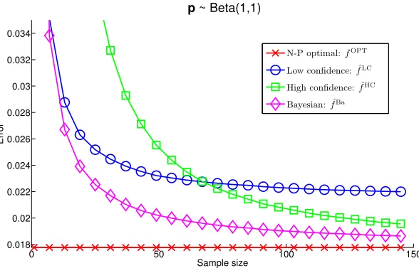
found it somewhat surprising that ˆfHC _{required so many samples (about 60 on}

average) to overtake ˆfLC_{. The simple majority rulef}MAJ _{(off the chart) performed}

at an average accuracy of 50%, as expected.

Bayesian setting. In each trial, a vector of expert competences p ∈ [0,1]n _{was drawn} independently componentwise, with pi ∼Beta(1,1). These values (i.e., αi =βi ≡1) were used for ˆfBa_{. The results are reported in Figure 2.}

7. Discussion

The classic and seemingly well-understood problem of the consistency of weighted majority votes continues to reveal untapped depth and suggest challenging unresolved questions. We hope that the results and open problems presented here will stimulate future research.

Acknowledgements

We thank Tony Jebara, Phil Long, Elchanan Mossel, and Boaz Nadler for enlightening discussions and for providing useful references. This paper greatly benefited from a careful reading by two diligent referees, who corrected inaccuracies and even supplied some new results. A special thanks to Lawrence Saul for writing up the new proof of the Kearns-Saul inequality and allowing us to print it here.

Appendix A. Bibliographical Notes on the Kearns-Saul Inequality

Given the recent interest surrounding the Kearns-Saul inequality (9), we find it instructive to provide some historical notes on this and related results. Most of the material in this section is taken from Saul (2014), to whom we are indebted for writing the note and for his kind permission to include it in this paper.

Lemma 19 Let f(x) = log cosh(1 2

√

x). Then f(x) is concave on x≥0.

Proof The second derivative is given by

f00(x) = sech

2₍1 2

√

x) 16x3/2

√

x−sinh(√x) .

For x > 0, the first of these factors is positive, and the second is negative. To show the latter, recall the Taylor series expansion

sinh(t) =t+ t

3

3!+

t5

5! +

t7

7!+. . . ,

from which we observe that √x ≤ sinh(√x). It also follows from the Taylor series that

f00_{(0) =−}1

96. It follows thatf

00 _{is negative on the positive half-line, and hencef is concave}

on this domain.

Corollary 20 Forx, x0 >0, we have

log cosh(1₂√x) ≤ log cosh(1₂√x0) +

"

tanh(1₂√x0)

4√x0

#

Proof A concave function f(x) is upper-bounded by its first-order Taylor approximation:

f(x)≤f(x0) +f0(x0)(x−x0). The claim follows from Lemma 19.

The results in Lemma 19 and Corollary 20 were first stated by Jaakkola and Jordan (1997); see Jebara (2011); Jebara and Choromanska (2012) for extensions, including a multivariate version. As pointed out by a referee, Theorem 1 in Hoeffding (1963) contains some bounds that bear a resemblance to the Kearns-Saul inequality. However, we were unable to derive the latter from the former — which, in particular, requires all of the summands to be bounded between 0 and 1.

Suppose that in Equation (53), we make the substitutions

√

x =

t+ log p 1−p

, (54)

√

x0 =

log p 1−p

, (55)

where t ∈ _R and p ∈ (0,1). Then we obtain a particular form of the bound that will be especially useful in what follows.

Corollary 21 For all t∈_Rand p∈(0,1),

log cosh

1 2

t+ log p 1−p

≤ −logh2pp(1−p)i+ (p−1₂)t+ 2p−1 4 log₁₋p_p

!

t2.

Proof Make the substitutions suggested in (54, 55) and apply Corollary 20. The result follows from tedious but elementary algebra.

The above result yields perhaps the most natural and direct proof of the Kearns-Saul inequality to date:

Theorem 22 For all t∈_Rand p∈(0,1),

logh(1−p)e−pt+pe(1−p)ti ≤ 2p−1

4 log₁₋p_p !

t2.

Proof Rewrite the left-hand side by symmetrizing the argument inside the logarithm,

logh(1−p)e−pt+pe(1−p)ti= log cosh

1 2

t+ log p 1−p

−(p−1₂)t+ logh2pp(1−p)i,

and invoke Corollary 21.

References

Jean-Yves Audibert, R´emi Munos, and Csaba Szepesv´ari. Tuning bandit algorithms in stochastic environments. InAlgorithmic Learning Theory (ALT), 2007.

Eyal Baharad, Jacob Goldberger, Moshe Koppel, and Shmuel Nitzan. Distilling the wisdom of crowds: weighted aggregation of decisions on multiple issues. Autonomous Agents and Multi-Agent Systems, 22(1):31–42, 2011.

Eyal Baharad, Jacob Goldberger, Moshe Koppel, and Shmuel Nitzan. Beyond Condorcet: Optimal aggregation rules using voting records. Theory and Decision, 72(1):113–130, 2012.

Daniel Berend and Aryeh Kontorovich. A sharp estimate of the binomial mean absolute deviation with applications. Statistics & Probability Letters, 83(4):1254–1259, 2013a.

Daniel Berend and Aryeh Kontorovich. On the concentration of the missing mass.Electron. Commun. Probab., 18:no. 3, 1–7, 2013b.

Daniel Berend and Aryeh Kontorovich. Consistency of weighted majority votes. In Neural Information Processing Systems (NIPS), 2014.

Daniel Berend and Jacob Paroush. When is Condorcet’s jury theorem valid? Soc. Choice Welfare, 15(4):481–488, 1998.

Daniel Berend and Luba Sapir. Monotonicity in Condorcet’s jury theorem with dependent voters. Social Choice and Welfare, 28(3):507–528, 2007.

Daniel Berend, Peter Harremo¨es, and Aryeh Kontorovich. Minimum KL-divergence on complements of L1 balls. IEEE Transactions on Information Theory, 60(6):3172–3177,

2014.

Philip J. Boland, Frank Proschan, and Y. L. Tong. Modelling dependence in simple and indirect majority systems. J. Appl. Probab., 26(1):81–88, 1989. ISSN 0021-9002.

Nicol`o Cesa-Bianchi and G´abor Lugosi. Prediction, Learning, and Games. Cambridge University Press, Cambridge, 2006.

Thomas M. Cover and Joy A. Thomas. Elements of information theory. Wiley-Interscience, Hoboken, NJ, second edition, 2006.

A. P. Dawid and A. M. Skene. Maximum likelihood estimation of observer error-rates using the EM algorithm. Applied Statistics, 28(1):20–28, 1979.

J.A.N. de Caritat marquis de Condorcet. Essai sur l’application de l’analyse `a la probabilit´e des d´ecisions rendues `a la pluralit´e des voix. AMS Chelsea Publishing Series. Chelsea Publishing Company, 1785.

Elad Eban, Elad Mezuman, and Amir Globerson. Discrete chebyshev classifiers. In Inter-national Conference on Machine Learning (ICML) (2), 2014.

Eyal Even-Dar, Sham M. Kakade, and Yishay Mansour. The value of observation for monitoring dynamic systems. InInternational Joint Conferences on Artificial Intelligence (IJCAI), 2007.

Yoav Freund and Robert E. Schapire. A decision-theoretic generalization of on-line learning and an application to boosting. J. Comput. Syst. Sci., 55(1):119–139, 1997.

Chao Gao and Dengyong Zhou. Minimax optimal convergence rates for estimating ground truth from crowdsourced labels (arxiv:1310.5764). 2014.

Trevor Hastie, Robert Tibshirani, and Jerome Friedman.The Elements of Statistical Learn-ing: Data Mining, Inference, and Prediction. Springer, New York, 2009.

David P. Helmbold and Philip M. Long. On the necessity of irrelevant variables. Journal of Machine Learning Research, 13:2145–2170, 2012.

Wassily Hoeffding. Probability inequalities for sums of bounded random variables.American Statistical Association Journal, 58:13–30, 1963.

Tommi S. Jaakkola and Michael I. Jordan. A variational approach to Bayesian logistic regression models and their extensions. InArtificial Intelligence and Statistics, AISTATS, 1997.

Tony Jebara. Multitask sparsity via maximum entropy discrimination. Journal of Machine Learning Research, 12:75–110, 2011.

Tony Jebara and Anna Choromanska. Majorization for CRFs and latent likelihoods. In

Neural Information Processing Systems (NIPS), 2012.

Michael J. Kearns and Lawrence K. Saul. Large deviation methods for approximate prob-abilistic inference. In Uncertainty in Artificial Intelligence (UAI), 1998.

Aryeh Kontorovich. Obtaining measure concentration from Markov contraction. Markov Processes and Related Fields, 4:613–638, 2012.

Aryeh (Leonid) Kontorovich. Measure Concentration of Strongly Mixing Processes with Applications. PhD thesis, Carnegie Mellon University, 2007.

Alexandre Lacasse, Fran¸cois Laviolette, Mario Marchand, Pascal Germain, and Nicolas Usunier. PAC-Bayes bounds for the risk of the majority vote and the variance of the Gibbs classifier. InNeural Information Processing Systems (NIPS), 2006.

Fran¸cois Laviolette and Mario Marchand. PAC-Bayes risk bounds for stochastic averages and majority votes of sample-compressed classifiers. Journal of Machine Learning Re-search, 8:1461–1487, 2007.

Hongwei Li, Bin Yu, and Dengyong Zhou. Error rate bounds in crowdsourcing models.

Nick Littlestone and Manfred K. Warmuth. The weighted majority algorithm. In Founda-tions of Computer Science (FOCS), 1989.

Nick Littlestone and Manfred K. Warmuth. The weighted majority algorithm.Inf. Comput., 108(2):212–261, 1994.

Yishay Mansour, Aviad Rubinstein, and Moshe Tennenholtz. Robust aggregation of experts signals. 2013.

Andreas Maurer and Massimiliano Pontil. Empirical Bernstein bounds and sample-variance penalization. InConference on Learning Theory (COLT), 2009.

David A. McAllester and Luis E. Ortiz. Concentration inequalities for the missing mass and for histogram rule error. Journal of Machine Learning Research, 4:895–911, 2003.

Volodymyr Mnih, Csaba Szepesv´ari, and Jean-Yves Audibert. Empirical Bernstein stop-ping. In International Conference on Machine Learning (ICML), 2008.

Jerzy Neyman and Egon S. Pearson. On the problem of the most efficient tests of statistical hypotheses. Philosophical Transactions of the Royal Society A: Mathematical, Physical and Engineering Sciences, 231(694-706):289–337, 1933.

Shmuel Nitzan and Jacob Paroush. Optimal decision rules in uncertain dichotomous choice situations. International Economic Review, 23(2):289–297, 1982.

Fabio Parisi, Francesco Strino, Boaz Nadler, and Yuval Kluger. Ranking and combining multiple predictors without labeled data. Proceedings of the National Academy of Sci-ences, 111(4):1253–1258, 2014.

Maxim Raginsky. Derivation of the Kearns-Saul inequality by optimal transportation (pri-vate communication), 2012.

Maxim Raginsky and Igal Sason. Concentration of measure inequalities in information theory, communications and coding. Foundations and Trends in Communications and Information Theory, 10(1-2):1–247, 2013.

Jean-Francis Roy, Fran¸cois Laviolette, and Mario Marchand. From PAC-Bayes bounds to quadratic programs for majority votes. InInternational Conference on Machine Learning (ICML), 2011.

Lawrence K. Saul. Yet another proof of an obscure inequality (private communication), 2014.

Robert E. Schapire and Yoav Freund. Boosting. Foundations and algorithms. Adaptive Computation and Machine Learning. Cambridge, MA: MIT Press, 2012.