Decision Boundary for Discrete Bayesian Network Classifiers

Decision Boundary for Discrete Bayesian Network Classifiers

Gherardo Varando [email protected]

Concha Bielza [email protected]

Pedro Larra˜naga [email protected]

Departamento de Inteligencia Artificial Universidad Polit´ecnica de Madrid Campus de Montegancedo, s/n

28660 Boadilla del Monte, Madrid, Spain

Editor:Max Chickering

Abstract

Bayesian network classifiers are a powerful machine learning tool. In order to evaluate the expressive power of these models, we compute families of polynomials that sign-represent decision functions induced by Bayesian network classifiers. We prove that those families are linear combinations of products of Lagrange basis polynomials. In absence ofV-structures in the predictor sub-graph, we are also able to prove that this family of polynomials does indeed characterize the specific classifier considered. We then use this representation to bound the number of decision functions representable by Bayesian network classifiers with a given structure.

Keywords: Bayesian networks, supervised classification, decision boundary, polynomial threshold function, Lagrange basis

1. Introduction

One of the problems with any supervised classification model, and Bayesian network clas-sifiers in particular, is to understand the limits of the expressive power of these models. The first rigorous result in this direction was reported by Minsky (1961), showing that the decision boundary in naive Bayes classifiers with binary predictors is a hyperplane. Since then several other researchers have addressed the problem. Peot (1996) reviewed Minsky’s results about binary predictors and presented some extensions. He mainly discussed the

case of naive Bayes with k-valued observations and observation-observation dependencies.

He also reported an upper bound on the number of linearly separable dichotomies of the

vertices of an n-dimensional cube, consequently bounding the number of decision functions

that are representable by naive Bayes classifiers with binary predictors. Domingos and Paz-zani (1997) studied the optimality of naive Bayes at length and pointed out that, even if the independence assumption among predictors is violated, naive Bayes could achieve optimal-ity under 0-1 loss. Jaeger (2003) showed, for binary predictors that, classifier expressivoptimal-ity at different levels of complexity is characterized by separability with polynomials of differ-ent degrees. Ling and Zhang (2002) reported negative results for the expressive power of

Bayesian networks; they proved that a Bayesian network where each node has at most k

studied the inner product space for Bayesian network classifiers with binary predictors, that is, the smallest Euclidean space that represents the induced concept class. They obtained upper and lower bounds on the dimension of the inner product space and they linked the dimension of the inner product space with the Vapnik-Chervonekis (VC) dimension (Vapnik and Chervonenkis, 1971). Yang and Wu (2012) studied the case of Bayesian networks with

k-valued nodes. They computed the VC dimension for fully connected Bayesian networks

and for Bayesian networks without V-structures. In both cases they showed that the VC

dimension is equal to the dimension of the inner product space.

In this paper we try to generalize the above results within a unified framework. To do this we compute polynomial threshold functions for Bayesian network (BN) binary classifiers in order to express their decision boundaries. This research is restricted to BN classifiers where the binary class variable,C, has no parents and where the predictors are categorical. As usual, our results extend to non-binary classifiers considering an ensemble of binary classifiers. Polynomial threshold functions are a way to describe the decision boundary of a discrete classifier and are a generalization of the results of Minsky (1961) and Peot (1996).

In absence of V-structures in the BN we prove that the obtained families of polynomial

representing the induced decision functions form linear spaces that are representations of the inner product spaces. We are able to compute the dimensions of those linear spaces and thus of the inner product space extending the results of Nakamura et al. (2005) and Yang and Wu (2012).

In Section 2 we define the notation used and briefly describe Bayesian network classi-fiers. In Section 3 we define a polynomial representation of the Iverson bracket (Iverson, 1962) over a finite number of categorical variables and derive the representation of discrete probability functions and of conditional probability tables. We then investigate polynomial representations of decision functions induced by Bayesian network classifiers. We look at Bayesian network classifiers in ascending order of complexity: naive Bayes classifiers in Sec-tion 3.2, tree augmented naive Bayes classifiers in SecSec-tion 3.3, Bayesian network-augmented naive Bayes classifiers in Section 3.4 and fully connected Bayesian network classifiers in Sec-tion 3.5. In SecSec-tion 4 we analyse the expressive power of BAN classifiers. Finally we present our conclusions and suggest possible future works in Section 5.

2. Preliminaries

We will use bold letters,xork, to represent elements of a product space, and letters with a

subscript to represent the respective components, for examplex2 indicates the second

com-ponent ofx. The capital letter P always refers to a probability, defined on an appropriate measure space, and capital letters X or X1, X2, Xi refer to random variables. For every

functionf : Ω→_Rand Ω0 ⊆Ω, we write f|Ω0 for the restriction of f over Ω0, that is, the

functionf|Ω0 : Ω0 →Rsuch thatf|Ω0(ξ) =f(ξ) for everyξ∈Ω0.

We consider a binary classification, that is, we are given a training set of labelled obser-vationsT =(x1, c1), . . . ,(xN, cN) , where xi = (xi₁, xi₂, . . . , xi_n)∈Ω⊂_Rn_{, with |Ω|<∞,}

and classes ci ∈ {−1,+1}. We search for a classification algorithm (classifier) Φ that, once trained on the setT, is able to classify every new instancex∈Ω into one of the two classes

clas-sifier Φ will classify each new instance xto class aiff_TΦ(x) =a. We drop the subscript T

since we are not interested in the relationship to the training set.

In this paper we focus on Bayes classifiers, probabilistic classifiers which learn from the training setT a joint probabilityP(X, C) and classify each new instancex= (x1, x2, . . . , xn)

in the most probable a posteriori class (MAP), that is,

fΦ(x) =argmax

c P(C=c|X=x) =argmaxc P(X=x, C =c).

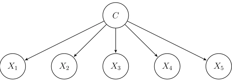
BN classifiers (Bielza and Larra˜naga, 2014) are Bayesian classifiers that factorize the joint probability distribution according to a Bayesian network. They range from the sim-plest naive Bayes classifier (Figure 1), where the predictor variables are assumed to be conditionally independent given the class variable, to the unrestricted Bayesian classifier, where a general form of Bayesian network (Pearl, 1988) is permitted. We will study only Bayesian network augmented naive Bayes classifiers, that is, we will consider the classCas a root node parent of every predictor variable. Once the structure of the Bayesian network is fixed, we need to estimate the parameters of the probability distribution. Thanks to the factorization implied by the Bayesian network structure we just estimate the conditional probability distributions of every variable given its parents, that is we have to estimate

P(Xi=xi|Xpa(i) =xpa(i)), whereXpa(i) stands for the vector of the parents ofXi. In the

discrete case this is reduced to the estimation of conditional probability tables. They could be estimated in several ways, but the straightforward approach using the maximum likeli-hood estimators (MLE), which are the relative frequencies, could lead to some conditional probabilities equal to zero. A Bayesian approach, such as the Laplace estimator or more generally Dirichlet-prior estimation of the parameters, will avoid this drawback. Because of this observation we will assume from now on that all parameters learned will be different from zero, that is, all the probabilities are positive.

To describe the complexity of decision functions we use the concept of threshold func-tions.

Definition 1 Given a decision function f : Ω → {−1,+1}, where Ω ⊂ _Rn_{, |Ω| < ∞}

and r : Rn 7→ R a polynomial we say that r sign-represents f or that f is computed by a

polynomial threshold function, if

f(x) =sgn(r(x)) for everyx∈Ω.

Moreover, given a set of polynomials P, we denote by sgn(P) the set of decision functions that are sign-representable by polynomials in P and by {−1,+1}Ω _{the set of all the 2}|Ω|

decision functions over Ω. Polynomial threshold functions are mainly studied in the theory of Boolean functions, functions g:{−1,+1}n_{→ {−1,+1} (O’Donnell and Servedio, 2010;}

Wang and Williams, 1991). A particular case is the linear threshold function, that is, when the degree of the polynomial that sign-represents the decision function is equal to one. Observe that different polynomials can sign-represent the same decision function, and not every polynomial sign-represents a decision function. In general we have that a polynomial

Example 1 Consider Ω = Ω1×Ω2, with Ω1 = {0,2,4} and Ω2 = {0,1}, and a decision

functionf : Ω→ {−1,+1} such that

f(x1, x2) =

(

−1 if (x1, x2)∈ {(0,0),(2,0),(4,1)}

+1 if (x1, x2)∈ {(0,1),(2,1),(4,0)}.

If we define polynomials

r(x1, x2) =−2x1x2+x1+ 6x2−3 q(x1, x2) =−2x2₁x2+x2₁+ 16x2−8,

we havesgn(r(x1, x2)) =sgn(q(x1, x2)) =f(x1, x2) for every(x1, x2)∈Ω, with r6=q, thus both polynomials sign-represent f.

If we consider a polynomial s(x1, x2) = x13+x2−8, we have that s(2,0) = 0 and thus s(x1, x2) cannot sign-represent any decision function over Ω.

3. Polynomial Threshold Functions for Bayesian Network Classifiers

We develop a method to easily compute polynomial threshold functions for Bayesian network classifiers. This method is an extension of the well-known results on the decision boundary of naive Bayes classifiers (Minsky, 1961; Peot, 1996). The method is based on the polynomial

interpolation of discrete probability functions or equivalently their logarithms. Pistone

et al. (2001) give a more formal and general description of this subject, also addressing applications to Bayesian networks. We will develop this method directly using Lagrange basis polynomials.

3.1 Lagrange Interpolation of Discrete Probability

The proofs of the results on the decision boundary in naive Bayes classifiers are based on a representation of the categorical distribution over two values{0,1} in an exponential form,

P(X = x) =px(1−p)1−x, with x ∈ {0,1} and p ∈ (0,1). We aim to reproduce the same representation for a categorical variable X ∈Λ = {ξ1, ξ2, . . . , ξm} ⊂_R, where the values of variableX are indicated as ξj withj as upper index. We consider{p(1), . . . , p(m)} such

thatPm

j=1p(j) = 1 and, using the Iverson bracket (Iverson, 1962), we write P(X =x) =

m

Y

j=1

p(j)[x=ξj]. (1)

IfX∈ {0,1}we could represent [x= 0] as 1−xand [x= 1] asx. If we consider a categorical variable, X∈Λ ={ξ1_{, ξ}2_{, . . . , ξ}m_{} ⊂}

R, we need to findmpolynomials

n

`Λ j

om

j=1 such that `Λ_j(ξj) = 1,

and

We easily see that such polynomials exist and have the following form:

`Λ_j(x) =Y

k6=j

(x−ξk)

(ξj _−ξk₎. (2)

The polynomials defined in Equation (2) are the Lagrange basis polynomials (Abramowitz and Stegun, 1964; Jeffreys and Jeffreys, 1999) over the points in Λ. These polynomials arem

linearly independent polynomials of degreem−1, and so they form a basis of polynomials

in one variable whose degree is at most m−1. We summarize some properties of these

polynomials in the following lemma.

Lemma 2 Let Ωi={ξ1i, ξi2, . . . , ξ mi

i } ⊂R, fori= 1, . . . , n. For everyidefine the Lagrange

basis, n

`Ωi_j (xi)

o

, over Ωi as in Equation (2). Then we have

1. For every i= 1, . . . , n, n`Ωi_j (xi)

omi

j=1 form a basis of the space of polynomials in xi of

degree |Ωi| −1.

2. Pmi₁ ji₁=1

Pmi₂ ji₂=1· · ·

Pmil j_il=1

Q

s∈I` Ωs js (xs) =

Q

i∈I

Pmi ji=1`

Ωi

ji(xi) = 1, for every x ∈ R I

and for all I ={i1, . . . , il} ⊆ {1, . . . , n}.

3. Q

i∈I` Ωi

ji (xi) = [xi = ξ ji

i ∀i ∈ I], for every I ⊆ {1, . . . , n}, for all {ji}i∈I such that

1≤ji≤mi, and for every x∈ ×i∈IΩi.

4. Pmi1

ji1=1

Pmi2

ji2=1· · ·

Pmip jip=1

Q

s∈I` Ωs js (xs) =

Q

i∈I\J` Ωi

ji (xi), for everyx∈R

I _{and for all}

J ={ii, . . . , ip} ⊂I ⊆ {1, . . . , n}.

Proof The proof of the above lemma is trivial, and we just outline some points. Point 1 fol-lows from the linear independences of the Lagrange basis polynomials. To prove point 2, we have merely to observe that, since

n

`Ωi_j

omi

j=1is a basis, we have that the polynomial constant

1 admits a unique representation in the considered basis, in particular 1 = Pmi

j=1` Ωi j (xi).

Point 3 follows trivially by substitution. To prove point 4 we apply point 2 as follows,

mi₁

X

ji₁=1 mi₂

X

ji₂=1

· · ·

mip

X

jip=1

Y

s∈I

`Ωs_js (xs) =





mi₁

X

ji₁=1 mi₂

X

ji₂=1

· · ·

mip

X

jip=1

Y

s∈J

`Ωs_js (xs)





| {z }

= 1

Y

i∈I\J `Ωi_j

i(xi) =

Y

i∈I\J `Ωi_j

i(xi).

If we are given a categorical random variableXover Λ ={ξ1, . . . , ξm}whose probability

mass function is P, we are able to rewrite Equation (1) using the Lagrange basis, as

P(X=x) =

m

Y

j=1

p(j)[x=ξj]=

m

Y

j=1

C

X

X

X

X

X

Figure 1: Naive Bayes classifier structure with five predictor variables

where p(j) =P(X =ξj) are the values of the probability mass function over Λ. Equation (3) is a consequence of the identity [x=ξj] =`Λ_j(x) which derives from point 3 of Lemma 2 considering|I|= 1. More generally, we consider a set of random variables{X1, X2, . . . , Xn}

such that, for every i = 1, . . . , n, the variable Xi ∈ Ωi ={ξ1i, ξi2, . . . , ξ mi

i }. If we are given

a conditional probability table that represents the probability function P(X1 = x1|X2 =

x2, . . . , Xn=xn), we can use the Iverson bracket overnvariablesx1, . . . , xnto describe the

conditional distribution ofX1 givenX2, . . . , Xn, P(X1 =x1|X2 =x2, . . . , Xn=xn) =

Y

(j1,...,jn)

p(j1|j2, . . . , jn)[xi=ξ ji

i ∀i=1,...,n]_,

where p(j1|j2, . . . , jn) = P(X1 = ξ1j1|X2 = ξ2j2, . . . , Xn = ξnjn) are the values of the

condi-tional probability table. Now using point 3 of Lemma 2 with I ={1, . . . , n}, we get

P(X1=x1|X2 =x2, . . . , Xn=xn) =

Y

(j1,...,jn)

p(j1|j2, . . . , jn) Qm

i=1` Ωi

ji(xi)_{. (4)}

3.2 Naive Bayes

We consider a naive Bayes classifier (NB) (Figure 1) where the predictor variablesXi ∈Ωi

are conditionally independent given the class variableC. The joint probability distribution factorizes as follows:

P(C=c, X1=x1, X2=x2, . . . , Xn=xn) =P(C =c) n

Y

i=1

P(Xi=xi|C=c). (5)

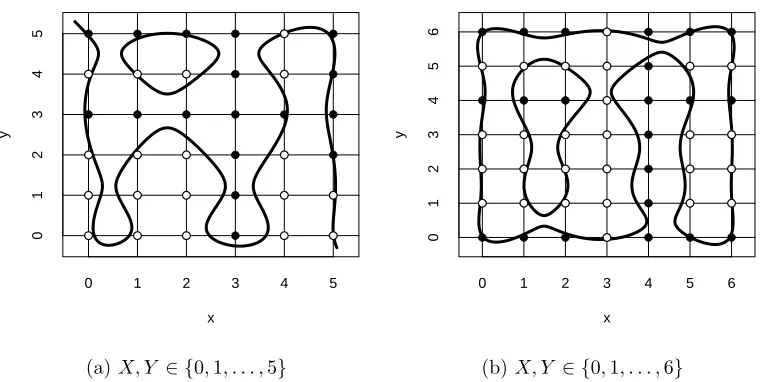
If the predictor variables are binary, Minsky (1961) proved that the decision boundaries are hyperplanes. For categorical predictors, the scenario is much more complicated as shown in Figure 2.

Theorem 3 A decision function f for a binary classification problem over n categorical variables Xi ∈ Ωi = {ξ1i, . . . , ξ

mi

i }, with |Ωi| = mi, is sign-represented by a polynomial of

the form Pn

i=1

Pmi

j=1αi(j)` Ωi j (xi)

if and only if there exists a naive Bayes classifier, with

x

y

0 1 2 3 4 5

0 1 2 3 4 5 ● ● ● ● ● ● ● ● ● ● ● ● ● ● ● ● ● ● ● ● ● ● ● ● ● ● ● ● ● ● ● ● ● ● ● ●

(a)X, Y ∈ {0,1, . . . ,5}

x

y

0 1 2 3 4 5 6

0 1 2 3 4 5 6 ● ● ● ● ● ● ● ● ● ● ● ● ● ● ● ● ● ● ● ● ● ● ● ● ● ● ● ● ● ● ● ● ● ● ● ● ● ● ● ● ● ● ● ● ● ● ● ● ●

(b)X, Y ∈ {0,1, . . . ,6}

Figure 2: Decision boundary for two example, (a) and (b), of naive Bayes classifiers with two categorical variablesX,Y. Boundaries are computed as location of zeroes of polynomials built as in Theorem 3

Proof We consider a naive Bayes classifier as in Figure 1. For every i = 1, . . . , n the variable Xi takes values over Ωi ={ξi1, . . . , ξ

mi

i }, a subset of R of cardinality mi. Thanks

to Equation (3), we can express, for every value c of the class, the conditional probability

P(Xi|C) as

P(Xi=xi|C =c) = mi

Y

j=1

pi(j|c)`

Ω_i

j (xi)_,

where pi(j|c) = P(Xi = ξ_ij|C = c). If we define ai(j|c) = ln(pi(j|c)), and assuming that pi(j|c)>0, we have that

P(Xi =xi|C =c) = exp





mi

X

j=1

ai(j|c)`Ωij (xi)



. (6)

Using this representation we easily find the decision function for NB with arbitrary discrete

predictor variables. Setting a= ln(P(C = +1)) and b = ln(P(C =−1)), we have that a

new instancex= (x1, . . . , xn) will be classified as C= +1 if

P(X1 =x1, . . . , Xn=xn, C= +1)> P(X1 =x1, . . . , Xn=xn, C=−1).

Using Equations (5) and (6) we have that the previous inequality could be rewritten as

exp 

a+

n X i=1   mi X j=1

ai(j|+ 1)`Ωi_j (xi)



 

>exp 

b+

n X i=1   mi X j=1

ai(j| −1)`Ωi_j (xi)



 

so the decision function for a naive Bayes classifier is

fN B(x) =sgn



a−b+

n X i=1   mi X j=1

α0_i(j)`Ωi_j (xi)



 

, (7)

whereα0i(j) =ai(j|+ 1)−ai(j| −1) = ln

P(Xi=ξj_i|C=+1) P(Xi=ξj_i|C=−1)

. We see from Equation (7) that

the decision function is sign-represented by a polynomial that admits the representation Pn

i=1

Pmi

j=1αi(j)`Ωij (xi)

. In fact we have that the a−b = lnP_P(_(CC=+1)₌₋₁₎ term could be included in the summation using Lemma 2, for example with the following choice of coefficient,

αi(j) = ln

P(Xi =ξij|C= +1) P(Xi =ξij|C=−1)

!

+kiln

P(C = +1)

P(C =−1)

, (8)

wherePn

i=1ki = 1. We have proved theif part of the theorem.

To prove the only if we have just to observe that choosing the conditional probabilities for the predictor variables given the class,P(Xi =ξ_ij|C =c), the probability mass for the

class P(C = +1) = 1−P(C = −1), and the values of {ki}ni=1 we are able to adjust the

coefficients αi(j) in (8) to any possible values in R. For example the following choices are

sufficient

P(Xi=ξj_i|C =−1) =

1

mi

∀i= 1, . . . , n and j= 1, . . . , mi,

P(Xi=ξji|C = +1) =

eαi(j)

Pmi j=1eαi(j)

∀i= 1, . . . , nand j= 1, . . . , mi,

ki =

ln_m1

i

Pmi j=1eαi(j)

Pn

i=1ln

1 mi

Pmi j=1eαi(j)

∀i= 1, . . . , n,

ln

P(C= +1)

P(C=−1) = n X i=1 ln   1 mi mi X j=1 eαi(j)



.

As a result of Theorem 3 we have that a naive Bayes classifier could represent every decision function which is sign-representable by a polynomial of the family







r(x) =

n X i=1   mi X j=1

αi(j)`Ωi_j (xi)



,αi(j)∈R







.

Only if we fix the prior probability over the class C are there restrictions on the coeffi-cientsαi(j).

Corollary 4 Let f be a decision function for a binary classification problem with n cat-egorical predictor variables Xi ∈ Ωi = {ξi1, . . . , ξ

mi

i } ⊂ R. The following sentences are

X1 C=−1 C= +1

0 0.3 0.3

1 0.1 0.2

2 0.4 0.1

3 0.1 0.2

4 0.1 0.2

X2 C =−1 C= +1

0 0.2 0.4

1 0.1 0.2

2 0.7 0.4

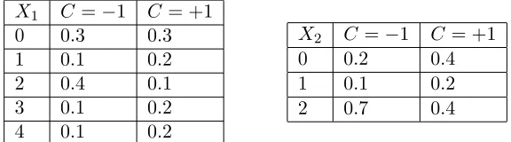
Table 1: Conditional Probability Tables in Example 2

i) f is sign-represented by a polynomial of the formPn

i=1

Pmi

j=1αi(j)`Ωij (xi)

withαi(j)

such that for every i = 1, . . . , n, there exists ji,1 and ji,2 such that αi(ji,1) < 0 and αi(ji,2)>0 or alternativelyeαi(j)= 1 for every j= 1, . . . , mi.

ii) There exists a naive Bayes classifier, with probability tables without zeros entries, that induces f, with uniform prior probability over the class C.

Proof The corollary follows from (8) in proof of Theorem 3, it is easy to show that the two conditions are equivalent.

As we can see, the coefficientsαi(j) are related to the probability model underlying the

problem, and are usually estimated from the training set but they do not generally assure the minimization of classification errors. An interesting model to deal with this problem is the weighted naive Bayes classifier (Webb and Pazzani, 1998; Hall, 2007). Weights are introduced in the probability factorization,

P(C=c|X=x)∝wcP(C =c) n

Y

i=1

[P(Xi =xi|C=c)]wi,

and thus the decision function has the same form as in (7), but with modified coefficients

αi(j) =wiln

P(Xi =j|C = +1) P(Xi =j|C =−1) .

Note that introducing the weights in the model does not change the form of the polynomial sign-representing the decision functions, so it does not improve the expressive power of the model. Even so, using the weighted model it is possible to search for polynomials that minimize the misclassification and improve accuracy (Zaidi et al., 2013). As future research it may be of some interest to study how to search polynomials to directly minimize the misclassification error and how this reflects on the implicitly defined NB classifier.

Example 2 We consider a naive Bayes classifier with two predictor variables X1 ∈Ω1 =

{0,1,2,3,4}andX2∈Ω2={0,1,2}. We have a uniform prior probability over the classC,

that is, P(C=−1) =P(C= +1) = 0.5, and we consider the conditional probability tables for X1 and X2 given in Table 1. We can directly build the polynomial threshold functions

α1(0) = ln0₀._.3₃ = 0 α2(0) = ln0₀._.4₂ = ln 2 α1(1) = ln0₀._.2₁ = ln 2 α2(1) = ln0₀._.2₁ = ln 2

α1(2) = ln0₀._.1₄ =−ln 4 α2(2) = ln0₀._.4₇ =−ln7₄ α1(3) = ln0₀._.2₁ = ln 2

α1(4) = ln0₀._.2₁ = ln 2

Table 2: Coefficients computations of polynomial (9)

coefficients are α1(j) = lnP(X1=j|C=+1)

P(X1=j|C=−1) and α2(j) = ln

P(X2=j|C=+1)

P(X2=j|C=−1), and the polynomial

r(x1, x2) is

r(x1, x2) =

4

X

j=0

α1(j)`Ω1

j (x1) + 2

X

j=0

α2(j)`Ω2

j (x2). (9)

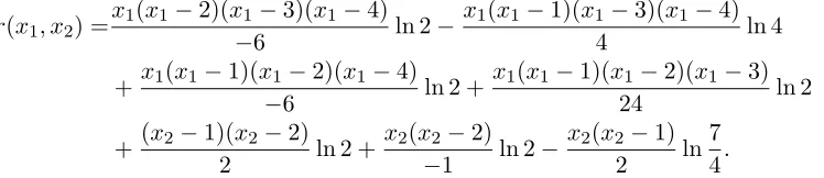
The computations of the coefficients are shown in Table 2. We have that the polynomial threshold function in Equation (9), expressed with the Lagrange basis, is

r(x1, x2) =x1(x1−2)(x1−3)(x1−4)

−6 ln 2−

x1(x1−1)(x1−3)(x1−4)

4 ln 4

+x1(x1−1)(x1−2)(x1−4)

−6 ln 2 +

x1(x1−1)(x1−2)(x1−3)

24 ln 2

+(x2−1)(x2−2)

2 ln 2 +

x2(x2−2)

−1 ln 2−

x2(x2−1)

2 ln

7 4.

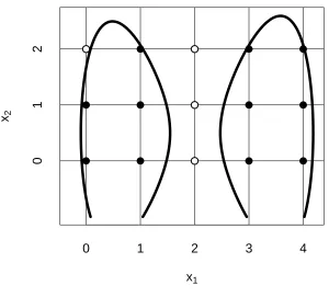
We observe that the above polynomial satisfies the condition of Corollary 4, as it should because the prior probability over C is uniform. Figure 3 shows the decision boundary induced by r(x1, x2).

3.3 Tree Augmented Naive Bayes

We now consider a tree augmented naive Bayes (TAN) classifier (Friedman et al., 1997) as shown in Figure 4. In this model, a predictor variable Xi ∈Ωi ={ξi1, . . . , ξ

mi

i } is allowed

to have at most two parents, the class C and an other variable, Xpa(i) ∈ Ωpa(i). The

joint probability distribution of (C, X1, X2, . . . , Xn) over {−1,+1} ×Ω1× · · · ×Ωn can be

factorized according to the Bayesian network theory as

P(C =c)

n

Y

i=1

P Xi =xi|C=c, Xpa(i)=xpa(i)

x₁

x2

0 1 2 3 4

0

1

2

● ● ●

● ● ●

● ● ●

● ● ●

● ● ●

Figure 3: Decision boundary for the naive Bayes structure of Example 2

C

X

X

X

X

X

C

X

X

X

X

X

Figure 5: SPODE Bayes classifier structure with five predictor variables

We can write down a similar representation to the NB case. For eachi= 1, . . . , n, we apply Equation (4) and obtain

P Xi=xi|C=c, Xpa(i)=xpa(i)

=

mi

Y

j=1 mpa(i)

Y

k=1

pi(j|c, k)

`Ω<sub>k</sub>pa(i)(xpa(i))` Ω_i

j (xi)

. (11)

We can now prove, combining Equations (10) and (11), a result similar to the NB case.

Lemma 5 If fT AN is the decision function induced by a TAN for a binary classification problem with n categorical predictor variables {Xi ∈ Ωi}n_i=1 and with probability tables

without zeros entries, then there exists a polynomial, of the form

n

X

i=1 mi

X

j=1

`Ωi_j (xi) mpa(i)

X

k=1

βi(j|k)` Ωpa(i)

k (xpa(i)),

that sign-represents fT AN, where we consider Pmpa(i)

k=1 βi(j|k)` Ωpa(i)

k (xpa(i)) = βi(j) when

Ω_pa(i)=∅, that is, when class C is the only parent of a node (the root node of the tree).

Proof The proof is a straightforward computation of the logarithm of Equation (10) using Equation (11) and the definition βi(j|k) = ln

pi(j|+1,k) pi(j|−1,k)

. The term corresponding to the

probability over the class ln

P(C=+1) P(C=−1)

could be made vanishing into the coefficients of the root nodeXtof the tree, using point 2 of Lemma 2 with I ={t}, with the following choice

of coefficients

βt(j) = ln

pi(j|+ 1) pi(j| −1)

+ ln

P(C= +1)

P(C=−1)

.

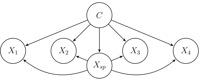
A particular case of TAN is the SuperParent-One-Dependence Estimator (SPODE)

(Keogh and Pazzani, 2002), where all the predictors depend on the same predictor (su-perparent) (Figure 5). The joint distribution factorizes as follows:

P(C=c)P(Xsp=xsp|C=c)

Y

i6=sp

where Xsp stands for the superparent node. In this case, the representation of Lemma 5

reduces to

fSP ODE(x) =sgn



 X

i6=sp mi

X

j=1

`Ωi_j (xi) msp

X

k=1

βi(j|k)` Ωsp k (xsp)



, (12)

wherefSP ODE _{is the induced decision function. If we fix the superparent node, we have a}

stronger characterization of the induced decision functions, the analogue of Theorem 3.

Theorem 6 A decision function for a binary classification problem over categorical predic-tor variables is sign-represented by a polynomial of the form

X

i6=sp mi

X

j=1

`Ωi_j (xi) msp

X

k=1

βi(j|k)`Ωsp_k (xsp),

if and only if it is induced by a SPODE classifier with Xsp as the superparent node and

with probability tables without zeros entries.

Proof The if part of the theorem is precisely Equation (12). To prove theonly if part we

repeat a similar argument as in Theorem 3. We observe (Lemma 2, point 4, with J ={i}

and I ={i, sp}) that for every i6=sp,

`Ωsp_k (xsp) = mi

X

j=1

`Ωi<sub>j</sub> (xi)` Ωsp k (xsp),

and so the coefficientβi(j|k) could be seen as

βi(j|k) = ln

P(Xi=j|Xsp =k, C = +1) P(Xi=j|Xsp =k, C =−1)

+αi(k),

whereP

i6=spαi(k) = ln

_P(Xsp=ξk sp|C=+1 P(Xsp=ξk

sp|C=−1

+αandα= ln_PP₍(C_C=+1)₌₋₁₎. Then adjustingαi(k)

and α properly we can find a SPODE model, that is, probability distributions over the

predictors and the class that induces

f =sgn



 X

i6=sp mi

X

j=1

`Ωi_j (xi) msp

X

k=1

βi(j|k)`Ωsp_k (xsp)



,

for everyβi(j|k)∈R.

Remark 8 Results similar to Theorem 6 could be proved whenever the structure of the predictor sub-graph of a TAN classifier is fixed. We expound no further theorems about TAN classifiers, as, in the next section, we will prove a more general result, of which NB and TAN are special cases.

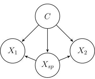
Example 3 We look at the SPODE model (see Figure 6 for structure) with the superparent node Xsp. We consider X1 ∈ {0,1,2}, X2 ∈ {0,1,2,3} and Xsp ∈ {0,1} with conditional

probability tables as shown in Table 3. The polynomial threshold function r(xsp, x1, x2) can

be computed directly as specified in Lemma 5:

r(xsp, x1, x2) = (1−xsp) ln

0.4 0.8

+xspln

0.6 0.2

+ (1−xsp)

(1−x1)(2−x1)

2 ln

0.2 0.1

+x1(2−x1) ln

0.7 0.1

+x1(x1−1)

2 ln

0.1 0.8

+xsp

(1−x1)(2−x1)

2 ln

0.7 0.3

+x1(2−x1) ln

0.1 0.2

+x1(x1−1)

2 ln

0.2 0.5

+ (1−xsp)

x2(2−x2)(3−x2)

2 ln

0.3 0.2

+x2(x2−1)(x2−2)

6 ln

0.1 0.2

+xsp

(1−x2)(2−x2)(3−x2)

6 ln

0.2 0.5

+x2(x2−1)(3−x2)

2 ln

0.5 0.2

.

We observe that some elements of the Lagrange bases do not appear inr(xsp, x1, x2) because

the corresponding coefficients are zero, since the conditional probabilities given C are equal.

3.4 Bayesian Network-Augmented Naive Bayes

If the predictor sub-graph can be a generic Bayesian network, we have a Bayesian network-augmented naive Bayes (BAN) classifier. In this case the joint probability distribution is factorized as follows:

P(C =c)

n

Y

i=1

P Xi =xi|C =c,Xpa(i)=xpa(i)

, (13)

where X_pa(i) denotes the vector of the parent variables of Xi that are not C. From now

on we will write pa(i) for the set of indexes definingXi’s parents that are notC andMi=

×_s∈pa(i){1, . . . , ms}for the set of possible configurations of the parents ofXi. Applying the

same arguments as in previous sections we can prove the lemma below.

Lemma 9 If fBAN is the decision function induced by a BAN classifier for a binary clas-sification problem with ncategorical predictors variables {Xi ∈Ωi ⊂R, |Ωi|=mi}ni=1 and

with probability tables without zeros entries, then there exists a polynomial of the form

n X i=1 mi X j=1

`Ωi_j (xi)

X

k∈_Mi

βi(j|k)

Y

s∈pa(i) `Ωs_k

s(xs),

which sign-represents fBAN, where we write P

k∈Miβi(j|k)

Q

s∈pa(i)` Ωs

ks(xs) = βi(j) when

C

X

X

X

Figure 6: SPODE classifier structure, Example 3

Xsp C=−1 C = +1

0 0.8 0.4

1 0.2 0.6

X1 C =−1 C= +1

Xsp = 0 Xsp= 1 Xsp = 0 Xsp= 1

0 0.1 0.3 0.2 0.7

1 0.1 0.2 0.7 0.1

2 0.8 0.5 0.1 0.2

X2 C=−1 C= +1

Xsp= 0 Xsp = 1 Xsp= 0 Xsp = 1

0 0.5 0.5 0.5 0.2

1 0.2 0.2 0.3 0.2

2 0.1 0.2 0.1 0.5

3 0.2 0.1 0.1 0.1

X

Y

Z

(a)

X

Y

Z

(b)

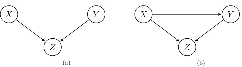
Figure 7: Graphical representation of (a) aV-structure and (b) an example which is not a

V-structure

Proof Given a BAN model over predictors Xi∈Ωi={ξi1, . . . , ξ mi

i }, we define

βi(j|k) = ln





PXi =ξij|C = +1, Xs=ξsks,∀s∈pa(i)

PXi =ξij|C =−1, Xs=ξsks,∀s∈pa(i)



.

Using Equation (4) and taking the logarithm of Equation (13) we obtain the polynomial representation. The additional constant term due to the prior probability over the class, ln

P(C=+1) P(C=−1)

, could be embedded into theβi(j|k) coefficients using point 2 of Lemma 2 as

in the proofs of Theorem 3 and Lemma 5.

Generally speaking, it is not always possible to prove results similar to Theorem 3 or Theorem 6 for BAN classifiers, when decision functions are completely characterized by the set of sign-representing polynomials. Like Yang and Wu (2012), we find that problems arise in the presence ofV-structures (Figure 7a) in the predictor sub-graph. A V-structure appears when two nodes share the same child, but are not directly connected. In absence of V-structures we can prove the following result, which extends the previous ones.

Theorem 10 Let G be a directed acyclic graph with node Xi for i = 1, . . . , n, and let f be a decision function for a binary classification problem over predictor variables Xi ∈

Ωi = {ξi1, . . . , ξ mi

i }. Suppose that G does not contain V-structures, then we have that f is

sign-represented by the following polynomial

r(x) =

n

X

i=1 mi

X

j=1

`Ωi_j (xi)

X

k∈_Mi

βi(j|k)

Y

s∈pa(i) `Ωs_k

s(xs),

if and only if f is induced by a BAN classifier whose predictor sub-graph is G and with probability tables without zeros entries.

Proof We merely have to prove theonly if because theif implication is precisely Lemma 9. Given a polynomial of the form

r(x) =

n

X

i=1

X

j∈Ωi

`Ωi_j (xi)

X

k∈_Mi

βi(j|k)

Y

s∈pa(i) `Ωs_k

we have to find a BAN classifier inducingsgn(r(x)), whose predictor sub-graph isG. We just have to define the conditional probability distribution of every variable given its parents, since the structure of the BAN is already fixed by G. For every i= 1, . . . , n, we observe that the sub-graph of the parents ofXi is a fully connected Bayesian network, otherwise we

will have aV-structure onG. For everyi, we can rewrite using point 4 of Lemma 2 the ith addend on the summation,

X

j∈Ωi

`Ωi_j (xi)

X

k∈Mi

βi(j|k)

Y

s∈pa(i) `Ωs_k

s(xs) +

X

k∈Mi αi(k)

Y

s∈pa(i) `Ωs_k

s(xs)−

X

k∈Mi αi(k)

Y

s∈pa(i) `Ωs_k

s(xs)

=X

j∈Ωi

`Ωi_j (xi)

X

k∈Mi

(βi(j|k) +αi(k))

Y

s∈pa(i)

`Ωs_ks(xs)−

X

k∈Mi αi(k)

Y

s∈pa(i)

`Ωs_ks(xs).

Using thefree parametersαi(k), it is possible to find for everyk,pi(j|k,+1) andpi(j|k,−1)∈

(0,1) such that

mi

X

j=1

pi(j|k,+1) = mi

X

j=1

pi(j|k,−1) = 1

βi(j|k) +αi(k) = ln

pi(j|k,+1) pi(j|k,−1) .

To avoid changing the polynomial r(x), we have to subtract X

k∈_Mi αi(k)

Y

s∈pa(i) `Ωs_k

s(xs)

from another addend on the summation. Because the parents ofXi are fully connected, we

have that among the other addends of r(x), apart from the ith, there is one product that

containsQ

s∈pa(i)` Ωs

ks(xs) and so we just subtractαi(k) from the related coefficient. Iterating

the above procedure for all the nodes of the graph G, we are able to build a probability

distribution over X1, X2, . . . , Xn, C that satisfies the Bayesian network structure given by

G. More precisely, setting

P

Xi=ξj_i|C=c, Xs=ξkss,∀s∈pa(i)

=pi(j|k, c),

we obtain the target BAN model.

We observe that the meaning of the representation in Theorem 10 is intuitive. If, as usual, we denote bypa(i) the function, dependent onG, that maps each variableXi to the

set of its parents, we have that a new instance x = (ξj1

1 , . . . , ξ jn

1 ) of the predictors will be

classified asC = +1 if and only if

r(x) =

n X i=1 mi X j=1 `Ωi_j (ξji

i )

X

k∈Mi

βi(j|k)

Y

s∈pa(i) `Ωs_k

s(ξ js s ) = n X i=1 `Ωi_ji(ξji

i )βi(ji|{js}s∈pa(i))

Y

s∈pa(i) `Ωs_js(ξjs

s )= n

X

i=1

In other words, every variableXi, together with its parentspa(i), expresses a degree

(posi-tive or nega(posi-tive)βi(ji|{js}s∈pa(i)) onx, based only on the values of thei-th variable,ξiki and

its parent values,{ξks

s ∀s∈pa(i)}. The degrees are summed, and a decision is taken based

on the result. The degree expressed by eachcoalition child-parents in the Bayesian network

classifier is the logarithm of the ratio between the two probabilities obtained conditioned on the values of the class C,

βi(ji|{js}s∈pa(i)) = ln

P(Xi =ξiji|Xs(i) =ξsjs,∀s∈pa(i), C = +1) P(Xi =ξiji|Xs(i) =ξsjs,∀s∈pa(i), C =−1) .

3.5 Full Bayesian Network

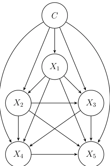
When the predictor sub-graph is a fully connected Bayesian network (Figure 8), that is, a directed acyclic graph with the maximum number of arcs, we have a fully connected Bayesian network classifier (FBN). A FBN can represent any joint probability distribu-tion over (C, X1, . . . , Xn) and so it is a classifier able to induce any decision function over

Ω = ×n

i=1Ωi whatsoever. We have that the product of the Lagrange bases,

Qn i=1`

Ωi ki(xi),

interpolates the Iverson bracket over all the predictors, that is,

n

Y

i=1 `Ωi_k

i(xi) = [xi=ξ ki

i ,∀i= 1, . . . , n].

And so the following lemma holds.

Lemma 11 If Φis a classifier for a binary class problem withncategorical predictor vari-ables X1, . . . , Xn such that Xi ∈ Ωi = {ξi1, . . . , ξ

mi

i } ⊂ R, |Ωi| = mi, then the associated

decision function, fΦ, is sign-represented by a polynomial of the form X

k∈M

γk

n

Y

i=1 `Ωi_k

i(xi),

where M=×ni=1{1, . . . , mi}.

We observe that the coefficients γk in Lemma 11 are the values of the polynomial at

point (ξk1

1 , ξ k2

2 , . . . , ξknn), and so fΦ(ξ k1

1 , ξ k2

2 , . . . , ξnkn) = sgn(γk). Roughly speaking, a new instance (ξk1

1 , ξ k2

2 , . . . , ξnkn) will be classified asC= +1 if and only if γk>0. Moreover the set

PF BN ₌

( X

k∈M

γk

n

Y

i=1 `Ωi_k

i(xi) s.t. γk∈R

)

of polynomials, which could sign-represent every classifier, is a space of dimension M =

|_M|=Qn

i=1mi. From now on we will write δk(x) =

n

Y

i=1 `Ωi_k

i(xi), (14)

for the k-th element of the canonical basis of PF BN_{. We call {δ}

k}k∈Ω the canonical basis

C

X

X

X

X

X

Figure 8: FBN classifier structure with five predictor variables

4. Expressive Power of Bayesian Network Classifiers

So far, we have seen how to build polynomial threshold functions that sign-represent decision functions induced by Bayesian network classifiers. We use now the resulting representation to bound the number of decision functions representable by Bayesian network classifiers.

As observed, Lemma 11 says that sgn(PF BN_{) = {−1,1}}Ω_{. We now study NB, SPODE}

and BAN through the families of associated polynomial threshold functions. Moreover,

we embed those families in PF BN_{. For predictor variables X}

i ∈ Ωi = {ξ1i, . . . , ξ mi i }, i =

1, . . . , n, for every sp∈ {1, . . . , n} and a directed acyclic graphG without V-structures we define

PN B = 





r(x) =

n

X

i=1





mi

X

j=1

αi(j)`Ωij (xi)



 s.t. α_i(j)∈R 





, (15)

P_spSP ODE = 





r(x) =X

i6=sp mi

X

j=1 msp

X

k=1

βi(j|k)` Ωsp

k (xsp)`Ωij (xi) s.t. βi(j|k)∈R







, (16)

P_GBAN = 





r(x) =

n

X

i=1 mi

X

j=1

`Ωi_j (xi)

X

k∈_Mi

βi(j|k)

Y

s∈pa(i) `Ωs_k

s(xs) s.t. βi(j|k)∈R







, (17)

wherepa(i) is a function that maps everyiinto the set of parents ofXiin the directed acyclic

of polynomials sign-representing the decision functions induced by naive Bayes classifier, SPODE classifier and BAN classifier, respectively. Hence sgn(PN B_{), sgn(P}SP ODE

sp ) and

sgn(PBAN

G ) are the sets of decision functions induced by naive Bayes, SPODE and BAN

classifiers, respectively. Obviously, we have that

PN B ⊂ P_GBAN ⊂ PF BN,

and

sgn(PN B_)⊂sgn(PBAN

G )⊂sgn(PF BN) ={−1,+1}Ω.

We can prove that the above sets are indeed subspaces ofPF BN _{and we can compute their}

dimensions.

Lemma 12 PN B _{is a subspace ofP}F BN _{of dimension} Pn

i=1mi−n+ 1. Proof Obviously PN B₌n_{p(x) =}Pn

i=1

Pmi

j=1αi(j)`Ωij (xi)

,αi(j)∈R

o

is a subspace of

PF BN_{. The union of the Lagrange bases over different variables is not a basis, because for}

each i= 1, . . . , n we have that

1 =

mi

X

j=1

`Ωi_j (xi) for everyxi ∈R.

So for everyi, we can define

Bi=







mi

[

j=2

{l_jΩi(xi)}







∪ {e0},

where e0 is the polynomial constant 1, and we find that Bi is a basis of polynomials in xi

of degree |Ωi| −1 =mi−1, equivalent to the Lagrange basis over Ωi. Then, we have that

B=

n

[

i=1

Bi = n

[

i=1 mi

[

j=2

n

lΩi_j (xi)

o

∪ {e0}

generates the subspacePN B_{. We prove thatBis in fact a basis ofP}N B_{. We have to prove}

that the elements ofB are linearly independent. We consider

p(x1, x2, . . . , xn) = n

X

i=1 mi

X

j=2

αi(j)`Ωij (xi) +α0e0= 0, ∀(x1, x2, . . . , xn)∈Rn.

If, as usual, Ωi ={ξi1, . . . , ξ mi

i }, let us consider p(x1, . . . , xn) evaluated in (ξ11, ξ21, . . . , ξn1),

0 =p(ξ1₁, ξ₂1, . . . , ξ_n1) =

n

X

i=1 mi

X

j=2

αi(j)`Ωij (ξ 1

i) +α0e0 =α0,

since`Ωi_j (ξ_i1) = 0 for everyj6= 1. And soα0 = 0. We now evaluatep(·) over (ξ₁j, ξ₂1, . . . , ξ_n1) and we have that, for every j= 2, . . . , mi,

since`Ω1

j (ξ j

1) = 1 for everyj= 2, . . . , m1. We repeat the above argument for every variable xi, i = 1, . . . , n and we obtain αi(j) = 0 for every i = 1, . . . , n and every j = 2, . . . , mi.

We have proved that the elements ofBgeneratePN B _{and are linearly independent, so they}

form a basis ofPN B_{. Consequently we obtain}

dim(PN B_{) =|B|=} n

X

i=1

mi−n+ 1.

Analogously we can prove, in the general case,

Lemma 13 For every Bayesian network classifier without V-structures in the predictor sub-graphG, the set PBAN

G is a subspace of PF BN of dimension

n

X

i=1



(mi−1)

Y

s∈pa(i) ms



+ 1.

And, in the particular case of SP ODE, we have,

Lemma 14 For everysp= 1, . . . , n, the set PSP ODE

sp is a subspace of PF BN of dimension msp

1−n+P

i6=spmi

.

We now consider the spacePF BN _{with respect to the canonical basis given by Equation}

(14). With respect to this coordinate system we have that each orthant represents a decision

function. We know that the number of orthants of an M-dimensional space is 2M, the

number of decision functions over a set of cardinality M. Since we now have a bijection

between orthants in PF BN _{and decision functions over Ω, in order to compute how many}

decision functions are representable by a class of Bayesian network classifier (NB, SPODE

or BAN) we merely have to count the number of orthants in PF BN _{intersected by the}

corresponding subspaces (PN B_,PSP ODE

sp ,PGBAN).

Theorem 15 (Flatto, 1970) Ad-dimensional subspace in anM-dimensional space inter-sects at mostC(M, d) = 2Pd−1

k=0 M−1

k

orthants with equality if and only if it is in general position.

Definition 16 Ad-dimensional subspaceV ofRM is in general position if theM subspaces

V ∩Hi, where Hi={x∈Rn s.t. xi = 0} are hyperplanes of V in general position, that

is, all the intersections of d of such hyperplanes are the zero vector. Precisely, for all

J ⊂ {1, . . . , M} such that |J|=dwe have that T

j∈J(V ∩Hj) =0.

Applying Theorem 15 to our case, we find that the spacePF BN _{is minimal in the following}

sense.

Corollary 17 IfV is a d-dimensional subspace ofPF BN_{, then|sgn(V)| ≤C(M, d), where} M =dim(PF BN_{) and equality holds if and only if V is in general position with respect to}

As a first result of Corollary 17 we have that the spacePF BN _{is thesmallest vector space of}

polynomials in x1, . . . , xnthat sign-represents every decision function over Ω, that is, there

is not a spaceV of polynomials inx1, . . . , xnwith degrees in each variablexithat are less or

equal thanmi−1 such thatsgn(V) ={−1,+1}Ωanddim(V)< dim(PF BN). This justifies

the choice ofPF BN _{as the space to study the polynomial families defined in Equations (15),}

(16) and (17). Next, we can use Corollary 17 combined with Lemma 13 to upper bound the number of decision functions that are sign-representable by BAN classifiers with a fixed

predictor sub-graph G not containingV-structures.

Corollary 18 Consider a BAN classifier over predictor variables Xi ∈ Ωi, |Ωi|= mi for

every i = 1, . . . , n. Moreover suppose that the predictor sub-graph G does not contain V -structures. Then we have

2d≤ |sgn(P_GBAN)| ≤C(M, d) = 2

d−1

X

k=0

M−1

k

,

where d=Pn

i=1

(mi−1)Qs∈pa(i)ms

+ 1and M =Qn

i=1mi.

Peot (1996) observed that naive Bayes could only represent a fraction of dichotomies (binary decision) on binary predictors, and that this fraction goes to zero as the number of

predictors increase, we extend this observation to BAN classifier without V-structures as

follows.

Corollary 19 We consider, for every n ∈N, classification problems with predictors Xi ∈

Ωi ⊂R, |Ωi|=mi for i= 1, . . . , n. For every n, let Gn be a directed acyclic graph over the

predictor variables, not containing V-structures. Suppose moreover that if pa_n(i) are the functions that map every Xi into the set of parents in the graph Gn,

|pa_n(i)| ≤K ∀n∈_N andi∈ {1, . . . , n},

then we have that

lim

n→∞

sgn P_GBAN

n

{−1,+1}Ω(n)

= lim

n→∞

sgn P_GBAN

n

2|Ω(n)| = 0,

where Ω(n) = ×n

i=1Ωi. In other words, the fraction of decision functions representable

by BAN classifiers, with a fixed maximum number of parents for each variable, becomes vanishingly small by increasing the number of predictors.

Proof For every n∈_N, we apply Corollary 18 and we obtain

sgn P_GBAN

n

≤C(M(n), d(n)) = 2

d(n)−1

X

k=0

M(n)−1

k

,

whered(n) =Pn

i=1

(mi−1)Qs∈pa(i)ms

+ 1 andM(n) =|Ω(n)|=Qn

i=1mi. We observe

now that, asn→ ∞,

d(n)

and thus,

C(M(n), d(n))

2M(n) →0,

which proves the statement.

5. Conclusions

In this paper we have shown how to build polynomial threshold functions related to Bayesian network classifiers. Our results reveal connections between the algebraic structure of the decision functions induced by BN classifiers and the topology of the structure of the predictor

sub-graph. In absence of V-structures in the predictor sub-graph we have also proved that

the specific polynomial representation fully characterized the type of Bayesian network

classifier. By representing classifiers by polynomial threshold functions, we can obtain

bounds on the number of decision functions which can be induced by Bayesian network

classifiers with a given structure. The bounding does not hold in presence of V-structures

in the predictor sub-graph. Strong characterizations of induced decision functions cannot be

proven due to the conditional independence of V-structure. Moreover we observe that the

obtained polynomial representation permits to easily prove the results of Ling and Zhang (2002) for BAN classifiers without V-structures.

The bounds points to the fact, already conjectured by Peot (1996) for naive Bayes, that if we fix the maximum number of parents in a Bayesian network classifier, the type of classifier considered is notscalable, in other words, more complex classifiers are expected to perform better when dealing with a large number of predictor variables.

Moreover, the resulting bounds for the number of decision functions representable are strictly upper bounds since the subspaces generated by the different Bayesian networks considered are not in general position. What happens in the case of subspaces not in general

position? Clearly we have to define some other property to characterize the position of a

subspace with respect to orthants in some given basis and try to count the number of such intersected orthants. With similar geometric results we will be able to precisely count the number of decision functions representable by a given Bayesian network classifier, and we will be able to compute the gain in expressivity from simple to more complicated Bayesian network classifiers.

Acknowledgments

References

Milton Abramowitz and Irene A. Stegun. Handbook of Mathematical Functions: With

Formulas, Graphs, and Mathematical Tables. Applied Mathematics Series. Dover Publi-cations, 1964.

Concha Bielza and Pedro Larra˜naga. Discrete Bayesian network classifiers: A survey. ACM

Comput. Surv., 47(1):5:1–5:43, 2014.

Pedro Domingos and Michael Pazzani. On the optimality of the simple Bayesian classifier

under zero-one loss. Machine Learning, 29(2-3):103–130, 1997.

Leopold Flatto. A new proof of the transposition theorem. Proceedings of the American

Mathematical Society, 24(1):29–31, 1970.

Nir Friedman, Dan Geiger, and Moises Goldszmidt. Bayesian network classifiers. Machine

Learning, 29(2-3):131–163, 1997.

Mark Hall. A decision tree-based attribute weighting filter for naive Bayes. In Max Bramer,

Frans Coenen, and Andrew Tuson, editors, Research and Development in Intelligent

Sys-tems XXIII, pages 59–70. Springer London, 2007.

Kenneth E. Iverson. A Programming Language. John Wiley & Sons, Inc., New York, 1962.

Manfred Jaeger. Probabilistic classifiers and the concepts they recognize. In Tom Fawcett

and Nina Mishra, editors,Proceedings of the Twentieth International Conference on

Ma-chine Learning (ICML-03), pages 266–273. AAAI Press, 2003.

Harold Jeffreys and Bertha Jeffreys. Methods of Mathematical Physics. Cambridge

Mathe-matical Library. Cambridge University Press, 1999.

Eamonn J. Keogh and Michael J. Pazzani. Learning the structure of augmented Bayesian classifiers. International Journal on Artificial Intelligence Tools, 11(04):587–601, 2002.

Charles X. Ling and Huajie Zhang. The representational power of discrete Bayesian

net-works. Journal of Machine Learning Research, 3:709–721, 2002.

Marvin Minsky. Steps toward artificial intelligence. In Computers and Thought, pages

406–450. McGraw-Hill, 1961.

Atsuyoshi Nakamura, Michael Schmitt, Niels Schmitt, and Hans Ulrich Simon. Inner

prod-uct spaces for Bayesian networks. Journal of Machine Learning Research, 6:1383–1403,

2005.

Ryan O’Donnell and Rocco A. Servedio. New degree bounds for polynomial threshold

functions. Combinatorica, 30(3):327–358, 2010.

Mark A. Peot. Geometric implications of the naive Bayes assumption. InProceedings of the Twelfth International Conference on Uncertainty in Artificial Intelligence, UAI’96, pages 414–419, San Francisco, 1996. Morgan Kaufmann Publishers Inc.

Giovanni Pistone, Eva Riccomagno, and Henry P. Wynn. Gr¨obner bases and factorisation

in discrete probability and Bayes. Statistics and Computing, 11(1):37–46, 2001.

Vladimir N. Vapnik and Alexy Chervonenkis. On the uniform convergence of relative

fre-quencies of events to their probabilities. Theory of Probability and Its Applications, 16

(2):264–280, 1971.

Chi Wang and A.C. Williams. The threshold order of a Boolean function. Discrete Applied

Mathematics, 31(1):51–69, 1991.

Geoffrey I. Webb and Michael J. Pazzani. Adjusted probability naive Bayesian induction. In Proceedings of the Eleventh Australian Joint Conference on Artificial Intelligence, pages 285–295. Springer-Verlag, 1998.

Youlong Yang and Yan Wu. On the properties of concept classes induced by multivalued

Bayesian networks. Information Sciences, 184(1):155–165, 2012.

Nayyar A. Zaidi, Jesus Cerquides, Mark J. Carman, and Geoffrey I. Webb. Alleviating naive

Bayes attribute independence assumption by attribute weighting. Journal of Machine