An Asynchronous Parallel Stochastic Coordinate Descent
Algorithm
Ji Liu [email protected]
Stephen J. Wright [email protected]
Department of Computer Sciences University of Wisconsin-Madison Madison, WI 53706-1685
Christopher R´e [email protected]
Department of Computer Science Stanford University
353 Serra Mall
Stanford, CA 94305-9025
Victor Bittorf [email protected]
Srikrishna Sridhar [email protected]
Department of Computer Sciences University of Wisconsin-Madison Madison, WI 53706-1685
Editor:Leon Bottou
Abstract
We describe an asynchronous parallel stochastic coordinate descent algorithm for mini-mizing smooth unconstrained or separably constrained functions. The method achieves a linear convergence rate on functions that satisfy an essential strong convexity property and a sublinear rate (1/K) on general convex functions. Near-linear speedup on a multicore system can be expected if the number of processors isO(n1/2) in unconstrained optimiza-tion andO(n1/4) in the separable-constrained case, wherenis the number of variables. We describe results from implementation on 40-core processors.
Keywords: asynchronous parallel optimization, stochastic coordinate descent
1. Introduction
Consider the convex optimization problem
min
x∈Ω f(x), (1)
where Ω⊂Rnis a closed convex set andf is a smooth convex mapping from an open neigh-borhood of Ω toR. We consider two particular cases of Ω in this paper: the unconstrained
case Ω =Rn, and the separable case
Formulations of the type (1,2) arise in many data analysis and machine learning prob-lems, for example, support vector machines (linear or nonlinear dual formulation) (Cortes and Vapnik, 1995), LASSO (after decomposing x into positive and negative parts) (Tib-shirani, 1996), and logistic regression. Algorithms based on gradient and approximate or partial gradient information have proved effective in these settings. We mention in partic-ular gradient projection and its accelerated variants (Nesterov, 2004), accelerated proximal gradient methods for regularized objectives (Beck and Teboulle, 2009), and stochastic gra-dient methods (Nemirovski et al., 2009; Shamir and Zhang, 2013). These methods are inherently serial, in that each iteration depends on the result of the previous iteration. Re-cently, parallel multicore versions of stochastic gradient and stochastic coordinate descent have been described for problems involving large data sets; see for example Niu et al. (2011); Richt´arik and Tak´aˇc (2012b); Avron et al. (2014).
This paper proposes an asynchronous stochastic coordinate descent (AsySCD) algo-rithm for convex optimization. Each step ofAsySCDchooses an indexi∈ {1,2, . . . , n}and subtracts a short, constant, positive multiple of the ith partial gradient∇if(x) :=∂f /∂xi from the ith component of x. When separable constraints (2) are present, the update is “clipped” to maintain feasibility with respect to Ωi. Updates take place in parallel across the cores of a multicore system, without any attempt to synchronize computation between cores. We assume that there is a boundτ on the age of the updates, that is, no more than τ updates toxoccur between the time at which a processor readsx(and uses it to evaluate one element of the gradient) and the time at which this processor makes its update to a single element of x. (A similar model of parallel asynchronous computation was used in Hogwild!(Niu et al., 2011).) Our implementation, described in Section 6, is a little more complex than this simple model would suggest, as it is tailored to the architecture of the Intel Xeon machine that we use for experiments.
We show that linear convergence can be attained if an “essential strong convexity” property (3) holds, while sublinear convergence at a “1/K” rate can be proved for general convex functions. Our analysis also defines a sufficient condition for near-linear speedup in the number of cores used. This condition relates the value of delay parameter τ (which relates to the number of cores / threads used in the computation) to the problem dimension n. A parameter that quantifies the cross-coordinate interactions in ∇f also appears in this relationship. When the Hessian of f is nearly diagonal, the minimization problem can almost be separated along the coordinate axes, so higher degrees of parallelism are possible. We review related work in Section 2. Section 3 specifies the proposed algorithm. Con-vergence results for unconstrained and constrained cases are described in Sections 4 and 5, respectively, with proofs given in the appendix. Computational experience is reported in Section 6. We discuss several variants ofAsySCDin Section 7. Some conclusions are given in Section 8.
1.1 Notation and Assumption
We use the following notation.
• ei∈Rndenotes theith natural basis vector (0, . . . ,0,1,0, . . . ,0)T with the ‘”1” in the
ith position.
• S⊂Ω denotes the set on whichf attains its optimal value, which is denoted byf∗.
• PS(·) and PΩ(·) denote Euclidean projection onto S and Ω, respectively.
• We use xi for the ith element of x, and ∇if(x) for the ith element of the gradient vector∇f(x).
• We define the following essential strong convexity condition for a convex function f with respect to the optimal setS, with parameterl > 0:
f(x)−f(y)≥ h∇f(y), x−yi+ l
2kx−yk
2 for allx, y∈Ω withP
S(x) =PS(y). (3)
This condition is significantly weaker than the usual strong convexity condition, which requires the inequality to hold forallx, y∈Ω. In particular, it allows for non-singleton solution setsS, provided thatf increases at a uniformly quadratic rate with distance from S. (This property is noted for convex quadratic f in which the Hessian is rank deficient.) Other examples of essentially strongly convex functions that are not strongly convex include:
– f(Ax) with arbitrary linear transformationA, wheref(·) is strongly convex;
– f(x) = max(aTx−b,0)2, fora6= 0.
• Define Lres as the restricted Lipschitz constant for∇f, where the “restriction” is to the coordinate directions: We have
k∇f(x)−∇f(x+tei)k ≤Lres|t|, for all i= 1,2, . . . , n and t∈R, with x, x+tei ∈Ω.
• DefineLi as thecoordinate Lipschitz constantfor∇f in theith coordinate direction: We have
f(x+tei)−f(x)≤ h∇if(x), ti+ Li
2 t
2, fori∈ {1,2, . . . , n}, and x, x+te i ∈Ω,
or equivalently
|∇if(x)− ∇if(x+tei)| ≤Li|t|.
• Lmax:= maxi=1,2,...,nLi. Note thatLres≥Lmax.
We use {xj}j=0,1,2,... to denote the sequence of iterates generated by the algorithm from starting point x0. Throughout the paper, we make the following assumption.
Assumption 1
• The optimal solution set S of (1) is nonempty.
• The radius of the iterate set {xj}j=0,1,2,... defined by R:= sup
j=0,1,2,...
kxj− PS(xj)k
1.2 Lipschitz Constants
The nonstandard Lipschitz constants Lres,Lmax, and Li, i= 1,2, . . . , n defined above are crucial in the analysis of our method. Besides bounding the nonlinearity off along various directions, these quantities capture the interactions between the various components in the gradient∇f, as quantified in the off-diagonal terms of the Hessian∇2f(x) — although the stated conditions do not require this matrix to exist.
We have noted already that Lres/Lmax≥1. Let us consider upper bounds on this ratio under certain conditions. Whenf is twice continuously differentiable, we have
Li = sup x∈Ω
max i=1,2,...,n[∇
2f(x)] ii.
Since ∇2f(x)0 for x∈Ω, we have that
|[∇2f(x)]ij| ≤
p
LiLj ≤Lmax, ∀i, j= 1,2, . . . , n.
Thus Lres, which is a bound on the largest column norm for ∇2f(x) over all x ∈ Ω, is bounded by √nLmax, so that
Lres Lmax
≤√n.
If the Hessian is structurally sparse, having at most p nonzeros per row/column, the same argument leads toLres/Lmax≤
√
p.
If f(x) is a convex quadratic with Hessian Q, we have
Lmax= max
i Qii, Lres= maxi kQ·ik2,
whereQ·idenotes theith column ofQ. IfQis diagonally dominant, we have for any column ithat
kQ·ik2≤Qii+k[Qji]j6=ik2 ≤Qii+
X
j6=i
|Qji| ≤2Qii,
which, by taking the maximum of both sides, implies thatLres/Lmax≤2 in this case. Finally, consider the objective f(x) = 12kAx−bk2 and assume that A ∈
Rm×n is a
random matrix whose entries are i.i.d fromN(0,1). The diagonals of the Hessian areAT·iA·i (where A·i is the ith column of A), which have expected value m, so we can expect Lmax to be not less than m. Recalling that Lresis the maximum column norm of ATA, we have
E(kATA·ik)≤E(|AT·iA·i|) +E(k[AT·jA·i]j6=ik) =m+E
s X
j6=i
|AT·jA·i|2
≤m+
s X
j6=i
E|AT·jA·i|2 =m+p(n−1)m,
where the second inequality uses Jensen’s inequality and the final equality uses
E(|AT·jA·i|2) =E(AT·jE(A·iA·Ti)A·j) =E(AT·jIA·j) =E(AT·jA·j) =m.
2. Related Work
This section reviews some related work on coordinate relaxation and stochastic gradient algorithms.
Among cyclic coordinate descent algorithms, Tseng (2001) proved the convergence of a block coordinate descent method for nondifferentiable functions with certain conditions. Local and global linear convergence were established under additional assumptions, by Luo and Tseng (1992) and Wang and Lin (2014), respectively. Global linear (sublinear) conver-gence rate for strongly (weakly) convex optimization was proved by Beck and Tetruashvili (2013). Block-coordinate approaches based on proximal-linear subproblems are described by Tseng and Yun (2009, 2010). Wright (2012) uses acceleration on reduced spaces (cor-responding to the optimal manifold) to improve the local convergence properties of this approach.
Stochastic coordinate descent is almost identical to cyclic coordinate descent except selecting coordinates in a random manner. Nesterov (2012) studied the convergence rate for a stochastic block coordinate descent method for unconstrained and separably constrained convex smooth optimization, proving linear convergence for the strongly convex case and a sublinear 1/K rate for the convex case. Extensions to minimization of composite functions are described by Richt´arik and Tak´aˇc (2012a) and Lu and Xiao (2013).
Synchronous parallel methodsdistribute the workload and data among multiple proces-sors, and coordinate the computation among processors. Ferris and Mangasarian (1994) proposed to distribute variables among multiple processors and optimize concurrently over each subset. The synchronization step searches the affine hull formed by the current iterate and the points found by each processor. Similar ideas appeared in (Mangasarian, 1995), with a different synchronization step. Goldfarb and Ma (2012) considered a multiple splitting algorithm for functions of the form f(x) = PN
k=1fk(x) in which N models are optimized separately and concurrently, then combined in an synchronization step. The alternating direction method-of-multiplier (ADMM) framework (Boyd et al., 2011) can also be imple-mented in parallel. This approach dissects the problem into multiple subproblems (possibly after replication of primal variables) and optimizes concurrently, then synchronizes to up-date multiplier estimates. Duchi et al. (2012) described a subgradient dual-averaging algo-rithm for partially separable objectives, with subgradient evaluations distributed between cores and combined in ways that reflect the structure of the objective. Parallel stochastic gradient approaches have received broad attention; see Agarwal and Duchi (2011) for an approach that allows delays between evaluation and update, and Cotter et al. (2011) for a minibatch stochastic gradient approach with Nesterov acceleration. Shalev-Shwartz and Zhang (2013) proposed an accelerated stochastic dual coordinate ascent method.
We turn now to asynchronous parallel methods. Bertsekas and Tsitsiklis (1989) intro-duced an asynchronous parallel implementation for general fixed point problems x =q(x) over a separable convex closed feasible region. (The optimization problem (1) can be formu-lated in this way by definingq(x) :=PΩ[(I−α∇f)(x)] for some fixedα >0.) Their analysis allows inconsistent reads forx, that is, the coordinates of the readx have different “ages.” Linear convergence is established if all ages are bounded and ∇2f(x) satisfies a diagonal dominance condition guaranteeing that the iterationx=q(x) is a maximum-norm contrac-tion mapping for sufficient small α. However, this condition is strong — stronger, in fact, than the strong convexity condition. For convex quadratic optimizationf(x) = 12xTAx+bx, the contraction condition requires diagonal dominance of the Hessian: Aii>Pi6=j|Aij|for all i= 1,2, . . . , n. By comparison,AsySCD guarantees linear convergence rate under the essential strong convexity condition (3), though we do not allow inconsistent read. (We require the vector x used for each evaluation of∇if(x) to have existed at a certain point in time.)
Hogwild! (Niu et al., 2011) is a lock-free, asynchronous parallel implementation of a stochastic-gradient method, targeted to a multicore computational model similar to the one considered here. Its analysis assumes consistent reading of x, and it is implemented without locking or coordination between processors. Under certain conditions, convergence ofHogwild!approximately matches the sublinear 1/K rate of its serial counterpart, which is the constant-steplength stochastic gradient method analyzed in Nemirovski et al. (2009). We also note recent work by Avron et al. (2014), who proposed an asynchronous linear solver to solve Ax = b where A is a symmetric positive definite matrix, proving a linear convergence rate. Both inconsistent- and consistent-read cases are analyzed in this paper, with the convergence result for inconsistent read being slightly weaker.
3. Algorithm
InAsySCD, multiple processors have access to a shared data structure for the vectorx, and each processor is able to compute a randomly chosen element of the gradient vector∇f(x). Each processor repeatedly runs the following coordinate descent process (the steplength parameterγ is discussed further in the next section):
R: Choose an index i∈ {1,2, . . . , n} at random, readx, and evaluate ∇if(x);
U: Update componentiof the sharedxby taking a step of lengthγ/Lmaxin the direction
−∇if(x).
Algorithm 1 Asynchronous Stochastic Coordinate Descent Algorithm xK+1 = AsySCD(x0, γ, K)
Require: x0 ∈Ω,γ, and K Ensure: xK+1
1: Initialize j←0;
2: whilej ≤K do
3: Choose i(j) from{1, . . . , n}with equal probability;
4: xj+1 ← PΩ
xj−Lmaxγ ei(j)∇i(j)f(xk(j))
;
5: j←j+ 1;
6: end while
The projection operation PΩ onto the feasible set is not needed in the case of uncon-strained optimization. For separable constraints (2), it requires a simple clipping operation on the i(j) component ofx.
We note several differences with earlier asynchronous approaches. Unlike the asyn-chronous scheme in Bertsekas and Tsitsiklis (1989, Section 6.1), the latest value of x is updated at each step, not an earlier iterate. Although our model of computation is similar to Hogwild! (Niu et al., 2011), the algorithm differs in that each iteration of AsySCD evaluates a single component of the gradient exactly, while Hogwild! computes only a (usually crude) estimate of the full gradient. Our analysis of AsySCD below is com-prehensively different from that of Niu et al. (2011), and we obtain stronger convergence results.
4. Unconstrained Smooth Convex Case
This section presents results about convergence of AsySCD in the unconstrained case Ω = Rn. The theorem encompasses both the linear rate for essentially strongly convex
f and the sublinear rate for general convex f. The result depends strongly on the delay parameterτ. (Proofs of results in this section appear in Appendix A.) In Algorithm 1, the indicesi(j),j= 0,1,2, . . . are random variables. We denote the expectation over all random variables as E, the conditional expectation in term of i(j) given i(0), i(1),· · ·, i(j−1) as Ei(j).
A crucial issue inAsySCDis the choice of steplength parameterγ. This choice involves a tradeoff: We would likeγ to be long enough that significant progress is made at each step, but not so long that the gradient information computed at step k(j) is stale and irrelevant by the time the update is applied at step j. We enforce this tradeoff by means of a bound on the ratio of expected squared norms on∇f at successive iterates; specifically,
ρ−1 ≤ Ek∇f(xj+1)k
2
Ek∇f(xj)k2
≤ρ, (4)
method at a linear rate, with rate constants that are almost consistent with vanilla short-step full-gradient descent.
Theorem 1 Suppose thatΩ =Rn in (1) and that Assumption 1 is satisfied. For anyρ >1,
define the quantityψ as follows:
ψ:= 1 + 2τ ρ τLres
√
nLmax
. (5)
Suppose that the steplength parameter γ >0 satisfies the following three upper bounds:
γ ≤ 1
ψ, (6a)
γ ≤ (ρ−1) √
nLmax 2ρτ+1L
res
, (6b)
γ ≤ (ρ−1) √
nLmax Lresρτ(2 +√nLLres
max)
. (6c)
Then we have that for anyj ≥0 that
ρ−1E(k∇f(xj)k2)≤E(k∇f(xj+1)k2)≤ρE(k∇f(xj)k2). (7)
Moreover, if the essentially strong convexity property (3) holds with l >0, we have
E(f(xj)−f∗)≤
1− 2lγ
nLmax
1−ψ
2γ
j
(f(x0)−f∗), (8)
while for general smooth convex functions f, we have
E(f(xj)−f∗)≤
1
(f(x0)−f∗)−1+jγ(1−ψ2γ)/(nLmaxR2)
. (9)
This theorem demonstrates linear convergence (8) for AsySCD in the unconstrained es-sentially strongly convex case. This result is better than that obtained forHogwild!(Niu et al., 2011), which guarantees only sublinear convergence under the stronger assumption of strict convexity.
The following corollary proposes an interesting particular choice of the parameters for which the convergence expressions become more comprehensible. The result requires a condition on the delay bound τ in terms of nand the ratioLmax/Lres.
Corollary 2 Suppose that Assumption 1 holds, and that
τ + 1≤ √
nLmax
2eLres . (10)
Then if we choose
ρ= 1 +√2eLres
nLmax
define ψ by (5), and setγ = 1/ψ, we have for the essentially strongly convex case (3) with
l >0 that
E(f(xj)−f∗)≤
1− l
2nLmax
j
(f(x0)−f∗), (12)
while for the case of general convexf, we have
E(f(xj)−f∗)≤
1
(f(x0)−f∗)−1+j/(4nLmaxR2). (13) We note that the linear rate (12) is broadly consistent with the linear rate for the classical steepest descent method applied to strongly convex functions, which has a rate constant of (1−2l/L), whereLis the standard Lipschitz constant for∇f. If we assume (not unreasonably) thatnsteps of stochastic coordinate descent cost roughly the same as one step of steepest descent, and note from (12) thatnsteps of stochastic coordinate descent would achieve a reduction factor of about (1−l/(2Lmax)), a standard argument would suggest that stochastic coordinate descent would require about 4Lmax/L times more computation. (Note that Lmax/L ∈ [1/n,1].) The stochastic approach may gain an advantage from the parallel implementation, however. Steepest descent requires synchronization and careful division of gradient evaluations, whereas the stochastic approach can be implemented in an asynchronous fashion.
For the general convex case, (13) defines a sublinear rate, whose relationship with the rate of the steepest descent for general convex optimization is similar to the previous para-graph.
As noted in Section 1, the parameter τ is closely related to the number of cores that can be involved in the computation, without degrading the convergence performance of the algorithm. In other words, if the number of cores is small enough such that (10) holds, the convergence expressions (12), (13) do not depend on the number of cores, implying that linear speedup can be expected. A small value for the ratio Lres/Lmax (not much greater than 1) implies a greater degree of potential parallelism. As we note at the end of Section 1, this ratio tends to be small in some important applications — a situation that would allow O(√n) cores to be used with near-linear speedup.
We conclude this section with a high-probability estimate for convergence of the sequence of function values.
Theorem 3 Suppose that the assumptions of Corollary 2 hold, including the definitions of
ρ and ψ. Then for any ∈(0, f(x0)−f∗) andη ∈(0,1), we have that
P(f(xj)−f∗ ≤)≥1−η, (14)
provided that either of the following sufficient conditions hold for the index j. In the essen-tially strongly convex case (3) with l >0, it suffices to have
j≥ 2nLmax
l
logf(x0)−f ∗
η
, (15)
while in the general convex case, a sufficient condition is
j ≥4nLmaxR2
1 η−
1 f(x0)−f∗
5. Constrained Smooth Convex Case
This section considers the case of separable constraints (2). We show results about conver-gence rates and high-probability complexity estimates, analogous to those of the previous section. Proofs appear in Appendix B.
As in the unconstrained case, the steplengthγ should be chosen to ensure steady progress while ensuring that update information does not become too stale. Because constraints are present, the ratio (4) is no longer appropriate. We use instead a ratio of squares of expected differences in successive primal iterates:
Ekxj−1−x¯jk2
Ekxj−x¯j+1k2
, (17)
where ¯xj+1 is the hypothesized full update obtained by applying the single-component update toevery component ofxj, that is,
¯
xj+1:= arg min
x∈Ωh∇f(xk(j)), x−xji+ Lmax
2γ kx−xjk 2. In the unconstrained case Ω =Rn, the ratio (17) reduces to
Ek∇f(xk(j−1))k2
Ek∇f(xk(j))k2 ,
which is evidently related to (4), but not identical.
We have the following result concerning convergence of the expected error to zero.
Theorem 4 Suppose that Ω has the form (2), that Assumption 1 is satisfied, and that
n≥5. Let ρ be a constant with ρ >(1−2/√n)−1, and define the quantity ψ as follows:
ψ:= 1 + Lresτ ρ τ
√
nLmax
2 +√Lmax
nLres + 2τ
n
. (18)
Suppose that the steplength parameter γ >0 satisfies the following two upper bounds:
γ ≤ 1
ψ, γ ≤
1−1
ρ − 2
√
n
√
nLmax
4Lresτ ρτ. (19)
Then we have
Ekxj−1−x¯jk2 ≤ρEkxj−x¯j+1k2, j= 1,2, . . . . (20)
If the essential strong convexity property (3) holds with l >0, we have for j= 1,2, . . . that
Ekxj− PS(xj)k2+ 2γ
Lmax(Ef(xj)−f
∗) (21)
≤
1− l
n(l+γ−1L max)
j
R2+ 2γ Lmax
(f(x0)−f∗)
.
For general smooth convex function f, we have
Ef(xj)−f∗ ≤
n(R2Lmax+ 2γ(f(x0)−f∗))
Similarly to the unconstrained case, the following corollary proposes an interesting par-ticular choice for the parameters for which the convergence expressions become more com-prehensible. The result requires a condition on the delay bound τ in terms of n and the ratioLmax/Lres.
Corollary 5 Suppose that Assumption 1 holds, that τ ≥1 and n≥5, and that
τ(τ + 1)≤ √
nLmax
4eLres . (23)
If we choose
ρ= 1 +√4eτ Lres
nLmax, (24)
then the steplength γ = 1/2 will satisfy the bounds (19). In addition, for the essentially strongly convex case (3) with l >0, we have for j = 1,2, . . . that
E(f(xj)−f∗)≤
1− l
n(l+ 2Lmax)
j
(LmaxR2+f(x0)−f∗), (25)
while for the case of general convexf, we have
E(f(xj)−f∗)≤
n(LmaxR2+f(x0)−f∗)
j+n . (26)
Similarly to Section 4, and providedτ satisfies (23), the convergence rate is not affected appreciably by the delay bound τ, and near-linear speedup can be expected for multicore implementations when (23) holds. This condition is more restrictive than (10) in the uncon-strained case, but still holds in many problems for interesting values ofτ. WhenLres/Lmax is bounded independently of dimension, the maximal number of cores allowed is of the the order ofn1/4, which is smaller than theO(n1/2) value obtained for the unconstrained case. We conclude this section with another high-probability bound, whose proof tracks that of Theorem 3.
Theorem 6 Suppose that the conditions of Corollary 5 hold, including the definitions of ρ
and ψ. Then for >0 and η∈(0,1), we have that
P(f(xj)−f∗ ≤)≥1−η,
provided that one of the following conditions holds: In the essentially strongly convex case (3) with l >0, we require
j≥ n(l+ 2Lmax)
l
logLmaxR
2+f(x0)−f∗ η
,
while in the general convex case, it suffices that
j≥ n(LmaxR
2+f(x
0)−f∗)
6. Experiments
We illustrate the behavior of two variants of the stochastic coordinate descent approach on test problems constructed from several data sets. Our interests are in the efficiency of multicore implementations (by comparison with a single-threaded implementation) and in performance relative to alternative solvers for the same problems.
All our test problems have the form (1), with either Ω = Rn or Ω separable as in (2).
The objectivef is quadratic, that is,
f(x) = 1 2x
TQx+cTx,
withQ symmetric positive definite.
Our implementation ofAsySCD is called DIMM-WITTED (or DW for short). It runs on various numbers of threads, from 1 to 40, each thread assigned to a single core in our 40-core Intel Xeon architecture. Cores on the Xeon architecture are arranged into four sockets — ten cores per socket, with each socket having its own memory. Non-uniform memory ac-cess (NUMA) means that memory acac-cesses to local memory (on the same socket as the core) are less expensive than accesses to memory on another socket. In our DW implementation, we assign each socket an equal-sized “slice” of Q, a row submatrix. The components of x are partitioned between cores, each core being responsible for updating its own partition of x(though it can read the components ofxfrom other cores). The components ofxassigned to the cores correspond to the rows of Q assigned to that core’s socket. Computation is grouped into “epochs,” where an epoch is defined to be the period of computation during which each component of x is updated exactly once. We use the parameter p to denote the number of epochs that are executed between reordering (shuffling) of the coordinates of x. We investigate both shuffling after every epoch (p = 1) and after every tenth epoch (p= 10). Access tox is lock-free, and updates are performed asynchronously. This update scheme does not implement exactly the “sampling with replacement” scheme analyzed in previous sections, but can be viewed as a high performance, practical adaptation of the AsySCD method.
To do each coordinate descent update, a thread must read the latest value of x. Most components are already in the cache for that core, so that it only needs to fetch those components recently changed. When a thread writes to xi, the hardware ensures that this xi is simultaneously removed from other cores, signaling that they must fetch the updated version before proceeding with their respective computations.
Although DW is not a precise implementation of AsySCD, it largely achieves the consistent-read condition that is assumed by the analysis. Inconsistent read happens on a core only if the following three conditions are satisfied simultaneously:
• A core does not finish reading recently changed coordinates of x (note that it needs to read no more thanτ coordinates);
• Among these recently changed coordinates, modifications take place both to coordi-nates thathave been read and that arestill to be read by this core;
Inconsistent read will occur only if at least two coordinates of x are modified twice during a stretch of approximately τ updates to x (that is, iterations of Algorithm 1). For the DW implementation, inconsistent read would require repeated updating of a particular component in a stretch of approximatelyτ iterations that straddles two epochs. This event would be rare, for typical values of nandτ. Of course, one can avoid the inconsistent read issue altogether by changing the shuffling rule slightly, enforcing the requirement that no coordinate can be modified twice in a span ofτ iterations. From the practical perspective, this change does not improve performance, and detracts from the simplicity of the approach. From the theoretical perspective, however, the analysis for the inconsistent-read model would be interesting and meaningful, and we plan to study this topic in future work.
The first test problem QP is an unconstrained, regularized least squares problem con-structed with synthetic data. It has the form
min x∈Rn
f(x) := 1
2kAx−bk 2+α
2kxk
2. (27)
All elements ofA∈Rm×n, the true model ˜x∈
Rn, and the observation noise vectorδ ∈Rm
are generated in i.i.d. fashion from the Gaussian distribution N(0,1), following which each column inAis scaled to have a Euclidean norm of 1. The observationb∈Rm is constructed
from A˜x+δkA˜xk/(5m). We choosem= 6000,n= 20000, and α= 0.5. We therefore have Lmax= 1 +α= 1.5 and
Lres Lmax ≈
1 +pn/m+α 1 +α ≈2.2.
This problem is diagonally dominant, and the condition (10) is satisfied when delay param-eterτ is less than about 95. In Algorithm 1, we set the steplength parameterγ to 1, and we choose initial iterate to be x0 =0. We measure convergence of the residual norm k∇f(x)k.
Our second problem QPcis a bound-constrained version of (27):
min x∈Rn +
f(x) := 1
2(x−x)˜
T(ATA+αI)(x−x).˜ (28)
The methodology for generatingA and ˜x and for choosing the values ofm,n,γ, and x0 is the same as for (27). We measure convergence via the residualkx− PΩ(x− ∇f(x))k, where Ω is the nonnegative orthant Rn+. At the solution of (28), about half the components of x are at their lower bound of 0.
Our third and fourth problems are quadratic penalty functions for linear programming relaxations of vertex cover problems on large graphs. The vertex cover problem for an undirected graph with edge set E and vertex set V can be written as a binary linear program:
min y∈{0,1}|V|
X
v∈V
yv subject to yu+yv ≥0, ∀(u, v)∈E.
By relaxing each binary constraint to the interval [0,1], introducing slack variables for the cover inequalities, we obtain a problem of the form
min yv∈[0,1], suv∈[0,1]
X
v∈V
This has the form
min x∈[0,1]n c
Tx subject to Ax=b,
for n=|V|+|E|. The test problem (29) is a regularized quadratic penalty reformulation of this linear program for some penalty parameter β:
min x∈[0,1]n c
Tx+ β
2kAx−bk 2+ 1
2βkxk
2, (29)
with β = 5. Two test data sets Amazon and DBLP have dimensions n = 561050 and n = 520891, respectively.
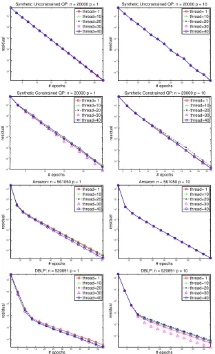
We tracked the behavior of the residual as a function of the number of epochs, when executed on different numbers of cores. Figure 1 shows convergence behavior for each of our four test problems on various numbers of cores with two different shuffling periods: p = 1 and p= 10. We note the following points.
• The total amount of computation to achieve any level of precision appears to be almost independent of the number of cores, at least up to 40 cores. In this respect, the performance of the algorithm does not change appreciably as the number of cores is increased. Thus, any deviation from linear speedup is due not to degradation of convergence speed in the algorithm but rather to systems issues in the implementation.
• When we reshuffle after every epoch (p= 1), convergence is slightly faster in synthetic unconstrainedQPbut slightly slower inAmazonandDBLP than when we do occasional reshuffling (p = 10). Overall, the convergence rates with different shuffling periods are comparable in the sense of epochs. However, when the dimension of the variable is large, the shuffling operation becomes expensive, so we would recommend using a large value forp for large-dimensional problems.
Results for speedup on multicore implementations are shown in Figures 2 and 3 for DW withp= 10. Speedup is defined as follows:
runtime a single core using DW runtime onP cores .
Near-linear speedup can be observed for the two QP problems with synthetic data. For Problems 3 and 4, speedup is at most 12-14; there are few gains when the number of cores exceeds about 12. We believe that the degradation is due mostly to memory contention. Although these problems have high dimension, the matrixQ is very sparse (in contrast to the dense Qfor the synthetic data set). Thus, the ratio of computation to data movement / memory access is much lower for these problems, making memory contention effects more significant.
Figures 2 and 3 also show results of a global-locking strategy for the parallel stochastic coordinate descent method, in which the vectorx is locked by a core whenever it performs a read or update. The performance curve for this strategy hugs the horizontal axis; it is not competitive.
5 10 15 20 25 30 10−4 10−3 10−2 10−1 100 101
Synthetic Unconstrained QP: n = 20000 p = 1
# epochs residual thread= 1 thread=10 thread=20 thread=30 thread=40
5 10 15 20 25 30 35 40 10−4 10−3 10−2 10−1 100 101
Synthetic Unconstrained QP: n = 20000 p = 10
# epochs residual thread= 1 thread=10 thread=20 thread=30 thread=40
5 10 15 20 25
10−5 10−4 10−3 10−2 10−1 100 101
Synthetic Constrained QP: n = 20000 p = 1
# epochs residual thread= 1 thread=10 thread=20 thread=30 thread=40
2 4 6 8 10 12 14 16 18 20 22
10−4 10−3 10−2 10−1 100 101
Synthetic Constrained QP: n = 20000 p = 10
# epochs residual thread= 1 thread=10 thread=20 thread=30 thread=40
10 20 30 40 50 60 70 80 90
10−4 10−3 10−2 10−1 100 101 102
Amazon: n = 561050 p = 1
# epochs residual thread= 1 thread=10 thread=20 thread=30 thread=40
10 20 30 40 50 60 70 10−4 10−3 10−2 10−1 100 101 102
Amazon: n = 561050 p = 10
# epochs residual thread= 1 thread=10 thread=20 thread=30 thread=40
5 10 15 20 25 30 35 40 45 50 10−3 10−2 10−1 100 101 102
DBLP: n = 520891 p = 1
# epochs residual thread= 1 thread=10 thread=20 thread=30 thread=40
5 10 15 20 25 30 35 40 10−3 10−2 10−1 100 101 102
DBLP: n = 520891 p = 10
# epochs residual thread= 1 thread=10 thread=20 thread=30 thread=40
5 10 15 20 25 30 35 40 5
10 15 20 25 30 35
40 Synthetic Unconstrained QP: n = 20000
threads
speedup
Ideal AsySCD−DW Global Locking
5 10 15 20 25 30 35 40
5 10 15 20 25 30 35
40 Synthetic Constrained QP: n = 20000
threads
speedup
Ideal AsySCD−DW Global Locking
Figure 2: Test problems 1 and 2: Speedup of multicore implementations of DW on up to 40 cores of an Intel Xeon architecture. Ideal (linear) speedup curve is shown for reference, along with poor speedups obtained for a global-locking strategy.
5 10 15 20 25 30 35 40 5
10 15 20 25 30 35 40
Amazon: n = 561050
threads
speedup
Ideal AsySCD−DW Global Locking
5 10 15 20 25 30 35 40
5 10 15 20 25 30 35 40
DBLP: n = 520891
threads
speedup
Ideal AsySCD−DW Global Locking
Figure 3: Test problems 3 and 4: Speedup of multicore implementations of DW on up to 40 cores of an Intel Xeon architecture. Ideal (linear) speedup curve is shown for reference, along with poor speedups obtained for a global-locking strategy.
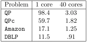
Problem 1 core 40 cores
QP 98.4 3.03
QPc 59.7 1.82
Amazon 17.1 1.25
DBLP 11.5 .91
Table 1: Runtimes (seconds) for the four test problems on 1 and 40 cores.
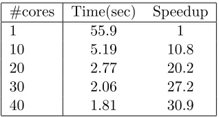
All problems reported on above are essentially strongly convex. Similar speedup prop-erties can be obtained in the weakly convex case as well. We show speedups for the QPc
problem with α = 0. Table 2 demonstrates similar speedup to the essentially strongly convex case shown in Figure 2.
#cores Time(sec) Speedup
1 55.9 1
10 5.19 10.8
20 2.77 20.2
30 2.06 27.2
40 1.81 30.9
Table 2: Runtimes (seconds) and speedup for multicore implementations of DW on different number of cores for the weakly convex QPc problem (with α = 0) to achieve a residual below 0.06.
#cores Time(sec) Speedup
SynGD/AsySCD SynGD/AsySCD
1 121. / 27.1 0.22 / 1.00
10 11.4 / 2.57 2.38 / 10.5 20 6.00 / 1.36 4.51 / 19.9 30 4.44 / 1.01 6.10 / 26.8 40 3.91 / 0.88 6.93 / 30.8
Table 3: Efficiency comparison between SynGD and AsySCD for the QP problem. The running time and speedup are based on the residual achieving a tolerance of 10−5.
Dataset # of # of Train time(sec) Samples Features LIBSVM AsySCD
adult 32561 123 16.15 1.39
news 19996 1355191 214.48 7.22
rcv 20242 47236 40.33 16.06
reuters 8293 18930 1.63 0.81
w8a 49749 300 33.62 5.86
Table 4: Efficiency comparison between LIBSVM and AsySCD for kernel SVM using 40 cores using homogeneous kernels (K(xi, xj) = (xTi xj)2). The running time and speedup are calculated based on the “residual” 10−3. Here, to make both algo-rithms comparable, the “residual” is defined bykx− PΩ(x− ∇f(x))k∞.
parallel, synchronous fashion, distributing the gradient computation load on multiple cores and updates the variable x in parallel at each step. The resulting implementation is called SynGD. Table 3 reports running time and speedup of bothAsySCDoverSynGD, showing a clear advantage forAsySCD.
reuterswere obtained from the LIBSVM data set repository.1 The data setreutersis a sparse binary text classification data set constructed as a one-versus-all version of Reuters-2159.2 Our comparisons, shown in Table 4, indicate thatAsySCDoutperforms LIBSVM on these test sets.
7. Extension
The AsySCD algorithm can be extended by partitioning the coordinates into blocks, and modifying Algorithm 1 to work with these blocks rather than with single coordinates. If Li,Lmax, and Lresare defined in the block sense, as follows:
k∇f(x)− ∇f(x+Eit)k ≤Lresktk ∀x, i, t∈R|i|,
k∇if(x)− ∇if(x+Eit)k ≤Liktk ∀x, i, t∈R|i|,
Lmax= max i Li,
whereEiis the projection from theith block toRnand|i|denotes the number of components
in blocki, our analysis can be extended appropriately.
To make the AsySCD algorithm more efficient, one can redefine the steplength in Algorithm 1 to be Lγ
i(j) rather than
γ
Lmax. Our analysis can be applied to this variant by
doing a change of variables to ˜x, withxi= LLmaxi x˜i and definingLi,Lres, and Lmaxin terms of ˜x.
8. Conclusion
This paper proposes an asynchronous parallel stochastic coordinate descent algorithm for minimizing convex objectives, in the unconstrained and separable-constrained cases. Sub-linear convergence (at rate 1/K) is proved for general convex functions, with stronger linear convergence results for functions that satisfy an essential strong convexity property. Our analysis indicates the extent to which parallel implementations can be expected to yield near-linear speedup, in terms of a parameter that quantifies the cross-coordinate inter-actions in the gradient ∇f and a parameter τ that bounds the delay in updating. Our computational experience confirms the theory.
Acknowledgments
This project is supported by NSF Grants DMS-0914524, DMS-1216318, and CCF-1356918; NSF CAREER Award IIS-1353606; ONR Awards N00014-13-1-0129 and N00014-12-1-0041; AFOSR Award FA9550-13-1-0138; a Sloan Research Fellowship; and grants from Oracle, Google, and ExxonMobil.
Appendix A. Proofs for Unconstrained Case
This section contains convergence proofs for AsySCD in the unconstrained case.
1.http://www.csie.ntu.edu.tw/~cjlin/libsvmtools/datasets/
We start with a technical result, then move to the proofs of the three main results of Section 4.
Lemma 7 For any x, we have
kx− PS(x)k2k∇f(x)k2≥(f(x)−f∗)2.
If the essential strong convexity property (3) holds, we have
k∇f(x)k2≥2l(f(x)−f∗). Proof The first inequality is proved as follows:
f(x)−f∗ ≤ h∇f(x), x− PS(x)i ≤ k∇f(x)kkPS(x)−xk.
For the second bound, we have from the definition (3), settingy←x and x← PS(x), that
f∗−f(x)≥ h∇f(x),PS(x)−xi+ l
2kx− PS(x)k 2 = l
2kPS(x)−x+ 1
l∇f(x)k 2− 1
2lk∇f(x)k
2≥ −1
2lk∇f(x)k 2, as required.
Proof (Theorem 1) We prove each of the two inequalities in (7) by induction. We start with the left-hand inequality. For all values ofj, we have
E k∇f(xj)k2− k∇f(xj+1)k2
=Eh∇f(xj) +∇f(xj+1),∇f(xj)− ∇f(xj+1)i
=Eh2∇f(xj) +∇f(xj+1)− ∇f(xj),∇f(xj)− ∇f(xj+1)i
≤2Eh∇f(xj),∇f(xj)− ∇f(xj+1)i
≤2E(k∇f(xj)kk∇f(xj)− ∇f(xj+1)k)
≤2LresE(k∇f(xj)kkxj−xj+1k)
≤ 2Lresγ
Lmax E
(k∇f(xj)kk∇i(j)f(xk(j))k)
≤ Lresγ
LmaxE
(n−1/2k∇f(xj)k2+n1/2k∇i(j)f(xk(j))k2) = Lresγ
LmaxE
(n−1/2k∇f(xj)k2+n1/2Ei(j)(k∇i(j)f(xk(j))k2)) = Lresγ
LmaxE
(n−1/2k∇f(xj)k2+n−1/2k∇f(xk(j))k2)
≤ √Lresγ
nLmaxE
k∇f(xj)k2+k∇f(xk(j))k2
. (30)
We can use this bound to show that the left-hand inequality in (7) holds for j = 0. By setting j= 0 in (30) and noting that k(0) = 0, we obtain
E k∇f(x0)k2− k∇f(x1)k2 ≤ √Lresγ
nLmax
From (6b), we have
2Lresγ
√
nLmax ≤ ρ−1
ρτ ≤ ρ−1
ρ = 1−ρ −1,
where the second inequality follows from ρ > 1. By substituting into (31), we obtain ρ−1E(k∇f(x0)k2) ≤ E(k∇f(x1)k2), establishing the result for j = 1. For the inductive step, we use (30) again, assuming that the left-hand inequality in (7) holds up to stage j, and thus that
E(k∇f(xk(j))k2)≤ρτE(k∇f(xj)k2),
provided that 0 ≤ j−k(j) ≤ τ, as assumed. By substituting into the right-hand side of (30) again, and usingρ >1, we obtain
E k∇f(xj)k2− k∇f(xj+1)k2
≤ 2Lresγρ
τ
√
nLmaxE k∇f(xj)k 2
.
By substituting (6b) we conclude that the left-hand inequality in (7) holds for all j. We now work on the right-hand inequality in (7). For all j, we have the following:
E k∇f(xj+1)k2− k∇f(xj)k2
=Eh∇f(xj) +∇f(xj+1),∇f(xj+1)− ∇f(xj)i
≤E(k∇f(xj) +∇f(xj+1)kk∇f(xj)− ∇f(xj+1)k)
≤LresE(k∇f(xj) +∇f(xj+1)kkxj−xj+1k)
≤LresE((2k∇f(xj)k+k∇f(xj+1)− ∇f(xj)k)kxj−xj+1k)
≤LresE(2k∇f(xj)kkxj−xj+1k+Lreskxj−xj+1k2)
≤LresE
2γ Lmax
k∇f(xj)kk∇i(j)f(xk(j))k+ Lresγ2
L2 max
k∇i(j)f(xk(j))k2
≤LresE
γ Lmax
(n−1/2k∇f(xj)k2+n1/2k∇i(j)f(xk(j))k2+ Lresγ2
L2 max
k∇i(j)f(xk(j))k2
=LresE
γ Lmax(n
−1/2k∇f(x
j)k2+n1/2Ei(j)(k∇i(j)f(xk(j))k2))+ Lresγ2
L2 max
Ei(j)(k∇i(j)f(xk(j))k2)
=LresE
γ Lmax
(n−1/2k∇f(xj)k2+n−1/2k∇f(xk(j))k2) + Lresγ2 nL2
max
k∇f(xk(j))k2
= √γLres
nLmaxE
k∇f(xj)k2+k∇f(xk(j))k2
+γ 2L2
res nL2
max
E(k∇f(xk(j))k2)
≤ √γLres
nLmaxE
(k∇f(xj)k2) +
γLres √ nLmax + γL 2 res nL2 max
E(k∇f(xk(j))k2), (32)
where the last inequality is from the observation γ ≤1. By setting j = 0 in this bound, and noting thatk(0) = 0, we obtain
E k∇f(x1)k2− k∇f(x0)k2≤
2γLres
√
nLmax + γL2res nL2
max
By using (6c), we have
2γLres
√
nLmax + γL
2 res nL2
max
= √Lresγ
nLmax
2 +√Lres
nLmax
≤ ρ−1
ρτ < ρ−1,
where the last inequality follows fromρ >1. By substituting into (33), we obtainE(k∇f(x1)k2)≤
ρE(k∇f(x0)k2), so the right-hand bound in (7) is established forj = 0. For the inductive step, we use (32) again, assuming that the right-hand inequality in (7) holds up to stagej, and thus that
E(k∇f(xj)k2)≤ρτE(k∇f(xk(j))k2),
provided that 0≤j−k(j)≤τ, as assumed. From (32) and the left-hand inequality in (7), we have by substituting this bound that
E k∇f(xj+1)k2− k∇f(xj)k2
≤
2γL√ resρτ nLmax +
γL2 resρτ nL2
max
E(k∇f(xj)k2). (34)
It follows immediately from (6c) that the term in parentheses in (34) is bounded above by ρ−1. By substituting this bound into (34), we obtain E(k∇f(xj+1)k2)≤ρE(k∇f(xj)k2), as required.
At this point, we have shown that both inequalities in (7) are satisfied for all j.
Next we prove (8) and (9). Take the expectation of f(xj+1) in terms of i(j):
Ei(j)f(xj+1) =Ei(j)f
xj− γ
Lmaxei(j)∇i(j)f(xk(j))
= 1 n
n
X
i=1 f
xj− γ Lmax
ei∇if(xk(j))
≤ 1
n n
X
i=1
f(xj)− γ
Lmaxh∇f(xj), ei∇if(xk(j))i+ Li 2L2
max
γ2k∇if(xk(j))k2
≤f(xj)− γ
nLmaxh∇f(xj),∇f(xk(j))i+ γ2
2nLmaxk∇f(xk(j))k 2 =f(xj) +
γ nLmax
h∇f(xk(j))− ∇f(xj),∇f(xk(j))i
| {z }
T1
−
γ nLmax −
γ2 2nLmax
The second term T1 is caused by delay. If there is no the delay issue, T1 should be 0 because of∇f(xj) =∇f(xk(j)). We estimate the upper bound ofk∇f(xk(j))− ∇f(xj)k:
k∇f(xk(j))− ∇f(xj)k ≤ j−1
X
d=k(j)
k∇f(xd+1)− ∇f(xd)k
≤Lres j−1
X
d=k(j)
kxd+1−xdk
= Lresγ Lmax
j−1
X
d=k(j)
∇i(d)f(xk(d))
. (36)
Then E(|T1|) can be bounded by
E(|T1|)≤E(k∇f(xk(j))− ∇f(xj)kk∇f(xk(j))k)
≤ Lresγ
LmaxE
j−1
X
d=k(j)
k∇i(d)f(xk(d))kk∇f(xk(j))k
≤ Lresγ 2LmaxE
j−1
X
d=k(j)
n1/2k∇i(d)f(xk(d))k2+n−1/2k∇f(xk(j))k2
= Lresγ 2LmaxE
j−1
X
d=k(j)
n1/2Ei(d)(k∇i(d)f(xk(d))k2) +n−1/2k∇f(xk(j))k2
= Lresγ 2LmaxE
j−1
X
d=k(j)
n−1/2k∇f(xk(d))k2+n−1/2k∇f(xk(j))k2
= Lresγ 2√nLmax
j−1
X
d=k(j)
E(k∇f(xk(d))k2+k∇f(xk(j))k2)
≤ τ ρ
τL resγ
√
nLmaxE
(k∇f(xk(j))k2) (37)
where the second line uses (36), and the final inequality uses the fact for d between k(j) and j−1, k(d) lies in the range k(j)−τ and j−1, so we have|k(d)−k(j)| ≤τ for all d.
Taking expectation on both sides of (35) in terms of all random variables, together with (37), we obtain
E(f(xj+1)−f∗)
≤E(f(xj)−f∗) + γ
nLmaxE(|T1|)−
γ nLmax − γ2 2nLmax
E(k∇f(xk(j))k2)
≤E(f(xj)−f∗)−
γ nLmax −
τ ρτLresγ2 n3/2L2
max
− γ
2 2nLmax
E(k∇f(xk(j))k2) =E(f(xj)−f∗)−
γ nLmax
1−ψ
2γ
which (because of (6a)) implies that E(f(xj) −f∗) is monotonically decreasing. From Lemma 7 and the assumption kxj− PS(xj)k ≤R for all j, we have
k∇f(xk(j))k2 ≥max
(
2l(f(xk(j))−f∗), (f(xk(j))−f ∗)2
kxk(j)− PS(xk(j))k2
)
≥max
(
2l(f(xk(j))−f∗), (f(xk(j))−f ∗)2 R2
)
,
which implies
E(k∇f(xk(j))k2)≥max
(
2lE(f(xk(j)−f∗),
E(f(xk(j)−f∗)2 R2
)
≥max
2lE(f(xj)−f∗), E
(f(xj)−f∗)2 R2
.
From the first upper boundk∇f(xk(j))k2≥2l
E(f(xj)−f∗), we have
E(f(xj+1)−f∗)≤E(f(xj)−f∗)− γ nLmax
1−ψ
2γ
E(k∇f(xk(j))k2)
≤
1− 2lγ
nLmax
1− ψ
2γ
E(f(xj)−f∗),
form which the linear convergence claim (8) follows by an obvious induction. From the
other boundk∇f(xk(j))k2 ≥
(f(xk(j))−f∗)2
R2 , we have
E(f(xj+1)−f∗)≤E(f(xj)−f∗)− γ nLmax
1−ψ
2γ
E(k∇f(xk(j))k2)
≤E(f(xj)−f∗)− γ nLmaxR2
1−ψ
2γ
E((f(xj)−f∗)2)
≤E(f(xj)−f∗)− γ nLmaxR2
1−ψ
2γ
(E(f(xj)−f∗))2, where the third line uses the Jensen’s inequalityE(v2)≥(E(v))2. Defining
C:= γ nLmaxR2
1−ψ
2γ
,
we have
E(f(xj+1)−f∗)≤E(f(xj)−f∗)−C(E(f(xj)−f∗))2
⇒ 1
E(f(xj)−f∗)
≤ 1
E(f(xj+1)−f∗)
−C E(f(xj)−f
∗)
E(f(xj+1)−f∗)
⇒ 1
E(f(xj+1)−f∗)
− 1
E(f(xj)−f∗)
≥C E(f(xj)−f
∗)
E(f(xj+1)−f∗)
≥C
⇒ 1
E(f(xj+1)−f∗)
≥ 1
f(x0)−f∗
+C(j+ 1)
⇒ E(f(xj+1)−f∗)≤
1
which completes the proof of the sublinear rate (9).
Proof (Corollary 2) Note first that for ρ defined by (11), we have
ρτ ≤ρτ+1=
1 +√2eLres
nLmax
√
nLmax 2eLres
2eL√res(τ+1) nLmax
≤e
2eL√res(τ+1)
nLmax ≤e,
and thus from the definition ofψ (5) that
ψ= 1 + 2τ ρ τL
res
√
nLmax ≤1 +
2τ eLres
√
nLmax ≤2. (38)
We show now that the steplength parameter choice γ = 1/ψ satisfies all the bounds in (6), by showing that the second and third bounds are implied by the first. For the second bound (6b), we have
(ρ−1)√nLmax 2ρτ+1Lres ≥
(ρ−1)√nLmax 2eLres ≥1≥
1 ψ,
where the second inequality follows from (11). For the third bound (6c), we have
(ρ−1)√nLmax Lresρτ(2 + √Lres
nLmax)
= 2eLres Lresρτ(2 +√Lres
nLmax)
≥ 2eLres
Lrese(2 +√Lres nLmax)
= 2
2 +√Lres nLmax
≥ 1
ψ.
We can thus setγ = 1/ψ, and by substituting this choice into (8) and using (38), we obtain (12). We obtain (13) by making the same substitution into (9).
Proof (Theorem 3) From Markov’s inequality, we have
P(f(xj)−f∗≥)≤−1E(f(xj)−f∗)
≤−1
1− l
2nLmax
j
(f(x0)−f∗)
≤−1(1−c)(1/c)
log
f(x0)−f∗ η
(f(x0)−f∗) withc=l/(2nLmax)
≤−1(f(x0)−f∗)e−
log
f(x0)−f∗ η
=ηelog
(f(x0)−f∗)
η e−
log
f(x0)−f∗ η
≤η,
where the second inequality applies (12), the third inequality uses the definition of j (15), and the second last inequality uses the inequality (1−c)1/c≤e−1 ∀c∈(0,1), which proves the essentially strongly convex case. Similarly, the general convex case is proven by
P(f(xj)−f∗ ≥)≤−1E(f(xj)−f∗)≤
f(x0)−f∗
1 +jf(x0)−f∗
4nLmaxR2 ≤η,
Appendix B. Proofs for Constrained Case
We start by introducing notation and proving several preliminary results. Define
(∆j)i(j):= (xj−xj+1)i(j), (39) and formulate the update in Step 4 of Algorithm 1 in the following way:
xj+1= arg min
x∈Ωh∇i(j)f(xk(j)),(x−xj)i(j)i+ Lmax
2γ kx−xjk 2.
(Note that (xj+1)i= (xj)i fori6=i(j).) From the optimality condition for this formulation, we have
(x−xj+1)i(j),∇i(j)f(xk(j))− Lmax
γ (∆j)i(j)
≥0, for all x∈Ω.
This implies in particular that for all x∈Ω, we have
(PS(x)−xj+1)i(j),∇i(j)f(xk(j))
≥ Lmax
γ
(PS(x)−xj+1)i(j),(∆j)i(j)
. (40)
From the definition of Lmax, and using the notation (39), we have
f(xj+1)≤f(xj) +h∇i(j)f(xj),−(∆j)i(j)i+ Lmax
2 k(∆j)i(j)k 2, which indicates that
h∇i(j)f(xj),(∆j)i(j)i ≤f(xj)−f(xj+1) + Lmax
2 k(∆j)i(j)k
2. (41)
From optimality conditions for this definition, we have
x−x¯j+1,∇f(xk(j)) + Lmax
γ (¯xj+1−xj)
≥0 ∀x∈Ω. (42)
We now define ∆j := xj −x¯j+1, and note that this definition is consistent with (∆)i(j) defined in (39). It can be seen that
Ei(j)(kxj+1−xjk2) = 1
nkx¯j+1−xjk 2. We now proceed to prove the main results of Section 5.
Proof (Theorem 4) We prove (20) by induction. First, note that for any vectorsa andb, we have
kak2− kbk2= 2kak2−(kak2+kbk2)≤2kak2−2ha, bi ≤2ha, a−bi ≤2kakka−bk, Thus for allj, we have
The second factor in the r.h.s. of (43) is bounded as follows:
kxj−x¯j+1−xj−1+ ¯xjk =
xj− PΩ(xj − γ Lmax
∇f(xk(j)))−(xj−1− PΩ(xj−1− γ Lmax
∇f(xk(j−1))))
≤
xj− γ Lmax
∇f(xk(j))− PΩ(xj − γ Lmax
∇f(xk(j)))−(xj−1− γ Lmax
∇f(xk(j−1))
−PΩ(xj−1− γ Lmax
∇f(xk(j−1))))
+ γ Lmax
∇f(xk(j−1))− ∇f(xk(j)) ≤
xj− γ
Lmax∇f(xk(j))−xj−1+ γ
Lmax∇f(xk(j−1))
+ γ Lmax
∇f(xk(j−1))− ∇f(xk(j))
≤ kxj−xj−1k+ 2 γ Lmax
∇f(xk(j))− ∇f(xk(j−1))
≤ kxj−xj−1k+ 2 γ Lmax
max{k(j−1),k(j)}−1
X
d=min{k(j−1),k(j)}
k∇f(xd)− ∇f(xd+1)k
≤ kxj−xj−1k+ 2 γLres Lmax
max{k(j−1),k(j)}−1
X
d=min{k(j−1),k(j)}
kxd−xd+1k, (44)
where the first inequality follows by adding and subtracting a term, and the second inequal-ity uses the nonexpansive property of projection:
k(z− PΩ(z))−(y− PΩ(y))k ≤ kz−yk.
One can see that j−1−τ ≤ k(j−1)≤ j−1 and j−τ ≤ k(j) ≤j, which implies that j−1−τ ≤d≤j−1 for each indexdin the summation in (44). It also follows that
max{k(j−1), k(j)} −1−min{k(j−1), k(j)} ≤τ. (45)
We set j = 1, and note that k(0) = 0 and k(1)≤ 1. Thus, in this case, we have that the lower and upper limits of the summation in (44) are 0 and 0, respectively. Thus, this summation is vacuous, and we have
kx1−x¯2+x0−x¯1k ≤
1 + 2γLres Lmax
kx1−x0k,
By substituting this bound in (43) and settingj = 1, we obtain
E(kx0−x1¯ k2)−E(kx1−x2¯ k2)≤
2 + 4γLres Lmax
For anyj, we have
E(kxj−xj−1kkx¯j−xj−1k)≤ 1 2E(n
1/2kx
j−xj−1k2+n−1/2kx¯j−xj−1k2) = 1
2E(n 1/2
Ei(j−1)(kxj−xj−1k2) +n−1/2kx¯j−xj−1k2) = 1
2E(n −1/2kx¯
j−xj−1k2+n−1/2kx¯j−xj−1k2)
=n−1/2Ekx¯j−xj−1k2. (47)
Returning to (46), we have
E(kx0−x1¯ k2)−E(kx1−x2¯ k2)≤2n−1/2Ekx1¯ −x0k2
which implies that
E(kx0−x1¯ k2)≤
1−√2
n −
4γLres
√
nLmax
−1
E(kx1−x2¯ k2)≤ρE(kx1−x2¯ k2).
To see the last inequality above, we only need to verify that
γ ≤
1−ρ−1−√2
n
√
nLmax 4Lres .
This proves that (20) holds for j= 1.
To take the inductive step, we assume that show that (20) holds up to indexj−1. We have for j−1−τ ≤d≤j−2 that
E(kxd−xd+1kkx¯j−xj−1k)≤ 1 2E(n
1/2kx
d−xd+1k2+n−1/2kx¯j −xj−1k2) = 1
2E(n 1/2
Ei(d)(kxd−xd+1k2) +n−1/2kx¯j−xj−1k2) = 1
2E(n −1/2kx
d−x¯d+1k2+n−1/2kx¯j −xj−1k2)
≤ 1
2E(n
−1/2ρτkx
j−1−x¯jk2+n−1/2kx¯j−xj−1k2)
≤ ρ
τ
n1/2E(kx¯j−xj−1k
where the second inequality uses the inductive hypothesis. By substituting (44) into (43) and taking expectation on both sides of (43), we obtain
E(kxj−1−x¯jk2)−E(kxj−x¯j+1k2)
≤2E(kx¯j−xj−1kkx¯j −x¯j+1+xj −xj−1k)
≤2E
kx¯j−xj−1k
kxj−xj−1k+ 2 γLres Lmax
max{k(j−1),k(j)}−1
X
d=min{k(j−1),k(j)}
kxd−xd+1k
= 2E(kx¯j−xj−1kkxj −xj−1k)+ 4γLres
Lmax
max{k(j−1),k(j)}−1
X
d=min{k(j−1),k(j)}
E(kx¯j−xj−1kkxd−xd+1k)
≤n−1/2
2 +4γLresτ ρ τ
Lmax
E(kxj−1−x¯jk2),
where the last line uses (45), (47), and (48). It follows that
E(kxj−1−x¯jk2)≤
1−n−1/2
2 +4γLresτ ρ τ
Lmax
−1
E(kxj−x¯j+1k2)≤ρE(kxj −x¯j+1k2).
To see the last inequality, one only needs to verify that
ρ−1≤1−√1
n
2 +4γLresτ ρ τ
Lmax
⇔ γ ≤
1−ρ−1−√2
n
√
nLmax 4Lresτ ρτ ,
and the last inequality is true because of the upper bound ofγ in (19). It proves (20). Next we will show the expectation of objective is monotonically decreasing. We have using the definition (39) that
Ei(j)(f(xj+1)) =n−1 n
X
i=1
f(xj+ (∆j)i)
≤n−1 n
X
i=1
f(xj) +h∇if(xj),(¯xj+1−xj)ii+ Lmax
2 k(xj+1−xj)ik 2
=f(xj) +n−1
h∇f(xj),x¯j+1−xji+ Lmax
2 kx¯j+1−xjk 2
=f(xj) + 1 n
h∇f(xk(j)),x¯j+1−xji+ Lmax
2 kx¯j+1−xjk 2
+ 1
nh∇f(xj)− ∇f(xk(j)),x¯j+1−xji
≤f(xj) + 1 n
Lmax
2 kx¯j+1−xjk
2−Lmax
γ kx¯j+1−xjk 2
+ 1
nh∇f(xj)− ∇f(xk(j)),x¯j+1−xji =f(xj)−
1 γ − 1 2 Lmax
n kx¯j+1−xjk 2+ 1
where the second inequality uses (42). Consider the expectation of the last term on the right-hand side of this expression. We have
Eh∇f(xj)− ∇f(xk(j)),x¯j+1−xji
≤Ek∇f(xj)− ∇f(xk(j))kkx¯j+1−xjk
≤E
j−1
X
d=k(j)
k∇f(xd)− ∇f(xd+1)kkx¯j+1−xjk
≤LresE
j−1
X
d=k(j)
kxd−xd+1kkx¯j+1−xjk
≤ Lres
2 E j−1
X
d=k(j)
(n1/2kxd−xd+1k2+n−1/2kx¯j+1−xjk2)
= Lres 2 E
j−1
X
d=k(j)
(n1/2Ei(d)(kxd−xd+1k2) +n−1/2kx¯j+1−xjk2)
= Lres 2 E
j−1
X
d=k(j)
(n−1/2kxd−x¯d+1k2+n−1/2kx¯j+1−xjk2)
≤ Lres
2n1/2E j−1
X
d=k(j)
(1 +ρτ)kx¯j+1−xjk2
≤ Lresτ ρ
τ
n1/2 Ekx¯j+1−xjk
2, (50)
where the fifth inequality uses (20). By taking expectation on both sides of (49) and substituting (50), we have
E(f(xj+1))≤E(f(xj))− 1 n
1 γ −
1 2
Lmax−
Lresτ ρτ n1/2
Ekx¯j+1−xjk2.
To see
1 γ −
1 2
Lmax−Lresτ ρτ
n1/2 ≥0, we only need to verify
γ ≤
1 2+
Lresτ ρτ
√
nLmax
−1
Next we prove the sublinear convergence rate for the constrained smooth convex case in (22). We have
kxj+1− PS(xj+1)k2≤ kxj+1− PS(xj)k2 =kxj −(∆j)i(j)ei(j)− PS(xj)k2
=kxj − PS(xj)k2+|(∆j)i(j)|2−2(xj − PS(xj))i(j)(∆j)i(j) =kxj − PS(xj)k2− |(∆j)i(j)|2−2 (xj− PS(xj))i(j)−(∆j)i(j)
(∆j)i(j) =kxj − PS(xj)k2− k(∆j)i(j)k2+ 2(PS(xj)−xj+1)i(j)(∆j)i(j)
≤ kxj − PS(xj)k2− |(∆j)i(j)|2+ 2γ Lmax
(PS(xj)−xj+1)i(j)∇i(j)f(xk(j)) =kxj − PS(xj)k2− |(∆j)i(j)|2+
2γ Lmax
(PS(xj)−xj)i(j)∇i(j)f(xk(j))+ 2γ
Lmax (∆j)i(j)∇i(j)f(xj) + (∆j)i(j) ∇i(j)f(xk(j))− ∇i(j)f(xj)
≤ kxj − PS(xj)k2− |(∆j)i(j)|2+ 2γ
Lmax(PS(xj)−xj)i(j)∇i(j)f(xk(j))+ 2γ
Lmax
f(xj)−f(xj+1) + Lmax
2 |(∆j)i(j)| 2
+ (∆j)i(j) ∇i(j)f(xk(j))− ∇i(j)f(xj)
=kxj − PS(xj)k2−(1−γ)|(∆j)i(j)|2+ 2γ
Lmax|(PS(xj)−xj){zi(j)∇i(j)f(xk(j)}) T1
+
2γ
Lmax(f(xj)−f(xj+1)) + 2γ
Lmax(∆j)i(j) ∇i(j)f(xk(j))− ∇i(j)f(xj)
| {z }
T2
where the second inequality uses (40) and the third inequality uses (41). We now seek upper bounds on the quantitiesT1 and T2 in the expectation sense. For T1, we have
E(T1) =n−1EhPS(xj)−xj,∇f(xk(j))i
=n−1EhPS(xj)−xk(j),∇f(xk(j))i+n−1E
j−1
X
d=k(j)
hxd−xd+1,∇f(xk(j))i =n−1EhPS(xj)−xk(j),∇f(xk(j))i
+n−1E
j−1
X
d=k(j)
hxd−xd+1,∇f(xd)i+hxd−xd+1,∇f(xk(j))− ∇f(xd)i
≤n−1E(f∗−f(xk(j))) +n−1E
j−1
X
d=k(j)
f(xd)−f(xd+1) + Lmax
2 kxd−xd+1k 2
+n−1E
j−1
X
d=k(j)
hxd−xd+1,∇f(xk(j))− ∇f(xd)i
=n−1E(f∗−f(xj)) + Lmax
2n E j−1
X
d=k(j)
kxd−xd+1k2
+n−1E
j−1
X
d=k(j)
hxd−xd+1,∇f(xk(j))− ∇f(xd)i
=n−1E(f∗−f(xj)) + Lmax
2n2 E j−1
X
d=k(j)
kxd−x¯d+1k2
+n−1E
j−1
X
d=k(j)
hxd−xd+1,∇f(xk(j))− ∇f(xd)i
≤n−1E(f∗−f(xj)) +
Lmaxτ ρτ
2n2 Ekxj−x¯j+1k 2
+n−1 j−1
X
d=k(j)
Ehxd−xd+1,∇f(xk(j))− ∇f(xd)i
| {z }
T3
where the last inequality uses (20). The upper bound of E(T3) is estimated by
E(T3) =Ehxd−xd+1,∇f(xk(j))− ∇f(xd)i =E(Ei(d)hxd−xd+1,∇f(xk(j))− ∇f(xd)i) =n−1Ehxd−x¯d+1,∇f(xk(j))− ∇f(xd)i
≤n−1Ekxd−x¯d+1kk∇f(xk(j))− ∇f(xd)k
≤n−1E(kxd−x¯d+1k d−1
X
t=k(j)
k∇f(xt)− ∇f(xt+1)k)
≤ Lres
n d−1
X
t=k(j)
E(kxd−x¯d+1kkxt−xt+1k)
≤ Lres
2n d−1
X
t=k(j)
E(n−1/2kxd−x¯d+1k2+n1/2kxt−xt+1k2)
≤ Lres
2n d−1
X
t=k(j)
E(n−1/2kxd−x¯d+1k2+n−1/2kxt−x¯t+1k2)
≤ Lresρ
τ
n3/2 d−1
X
t=k(j)
E(kxj−x¯j+1k2)
≤ Lresτ ρ
τ
n3/2 E(kxj−x¯j+1k 2).
where the second last inequality uses (20). Therefore, E(T1) can be bounded by
E(T1) =Eh(PS(xj)−xj)i(j),∇i(j)f(xk(j))i
≤ 1
nE(f
∗−f(x
j)) +
Lmaxτ ρτ
2n2 Ekxj−x¯j+1k 2+
j−1
X
d=k(j)
Lresτ ρτ
n5/2 E(kxj−x¯j+1k 2)
= 1 n
f∗−Ef(xj) +
Lmaxτ ρτ 2n +
Lresτ2ρτ n3/2
E(kxj−x¯j+1k2)
For T2, we have
E(T2) =E(∆j)i(j) ∇i(j)f(xk(j))− ∇i(j)f(xj)
=n−1Eh∆j,∇f(xk(j))− ∇f(xj)i
≤n−1E(k∆jkk∇f(xk(j))− ∇f(xj)k)
≤n−1E
j−1
X
d=k(j)
k∆jkk∇f(xd)− ∇f(xd+1)k
≤ Lres n E
j−1
X
d=k(j)
k∆jkkxd−xd+1k
= Lres 2n E
j−1
X
d=k(j)
n−1/2k∆jk2+n1/2kxd−xd+1k2
= Lres 2n E
j−1
X
d=k(j)
n−1/2kxj −x¯j+1k2+n1/2Ei(d)kxd−xd+1k2
= Lres 2n E
j−1
X
d=k(j)
n−1/2kxj −x¯j+1k2+n−1/2kxd−x¯d+1k2
= Lres 2n3/2
j−1
X
d=k(j)
Ekxj−x¯j+1k2+Ekxd−x¯d+1k2
≤ Lres(1 +ρ
τ)
2n3/2
j−1
X
d=k(j)
Ekxj−x¯j+1k2
≤ Lresτ ρ
τ
n3/2 Ekxj−x¯j+1k
2, (53)
where the second last inequality uses (20).
By taking the expectation on both sides of (51), using Ei(j)(|(∆j)i(j)|2) = n−1kxj − ¯
xj+1k2, and substituting the upper bounds from (52) and (53), we obtain
Ekxj+1− PS(xj+1)k2 ≤Ekxj− PS(xj)k2
− 1
n
1−γ−2γLresτ ρ
τ
Lmaxn1/2 − γτ ρτ
n −
2γLresτ2ρτ Lmaxn3/2
Ekxj−x¯j+1k2 + 2γ
Lmaxn
(f∗−Ef(xj)) + 2γ Lmax
(Ef(xj)−Ef(xj+1))
≤Ekxj− PS(xj)k2+ 2γ Lmaxn(f
∗−
Ef(xj)) + 2γ
Lmax(Ef(xj)−Ef(xj+1)). (54) In the second inequality, we were able to drop the term involving Ekxj−x¯j+1k2 by using the fact that
1−γ−2γLresτ ρ
τ
Lmaxn1/2 − γτ ρτ
n −
2γLresτ2ρτ
which follows from the definition (18) of ψand from the first upper bound on γ in (19). It follows that
Ekxj+1− PS(xj+1)k2+ 2γ
Lmax(Ef(xj+1)−f ∗)
≤Ekxj − PS(xj)k2+ 2γ Lmax
(Ef(xj)−f∗)− 2γ Lmaxn
(Ef(xj)−f∗) (55)
≤ kx0− PS(x0)k2+ 2γ
Lmax(f(x0)−f
∗)− 2γ Lmaxn
j
X
t=0
(Ef(xt)−f∗)
≤R2+ 2γ
Lmax(f(x0)−f ∗
)−2γ(j+ 1)
Lmaxn (Ef(xj+1)−f ∗
),
where the second inequality follows by applying induction to the inequality
Sj+1 ≤Sj− 2γ LmaxnE
(f(xj)−f∗),
where
Sj :=E(kxj− PS(xj)k2) + 2γ LmaxE
(f(xj)− PS(xj)),
and the last line uses the monotonicity of Ef(xj) (proved above) and the assumed bound
kx0− PS(x0)k ≤R. It implies that
Ekxj+1− PS(xj+1)k2+ 2γ Lmax
(Ef(xj+1)−f∗) +
2γ(j+ 1) Lmaxn
(Ef(xj+1)−f∗)
≤R2+ 2γ
Lmax
(f(x0)−f∗)
⇒ 2γ(n+j+ 1)
Lmaxn
(Ef(xj+1)−f∗)≤R2+ 2γ Lmax
(f(x0)−f∗)
⇒Ef(xj+1)−f∗ ≤
n(R2Lmax+ 2γ(f(x0)−f∗)) 2γ(n+j+ 1) .
This completes the proof of the sublinear convergence rate (22).
Finally, we prove the linear convergence rate (21) for the essentially strongly convex case. All bounds proven above hold, and we make use the following additional property:
f(xj)−f∗ ≥ h∇f(PS(xj)), xj− PS(xj)i+ l
2kxj− PS(xj)k 2 ≥ l
2kxj− PS(xj)k 2, due to feasibility of xj and h∇f(PS(xj)), xj − PS(xj)i ≥0. By using this result together with some elementary manipulation, we obtain
f(xj)−f∗=
1− Lmax
lγ+Lmax
(f(xj)−f∗) +
Lmax lγ+Lmax
(f(xj)−f∗)
≥
1− Lmax
lγ+Lmax
(f(xj)−f∗) +
Lmaxl 2(lγ+Lmax)
kxj − PS(xj)k2 = Lmaxl
2(lγ+Lmax)
kxj− PS(xj)k2+ 2γ
Lmax(f(xj)−f ∗)