On the Influence of Momentum Acceleration on Online
Learning
Kun Yuan [email protected]
Bicheng Ying [email protected]
Ali H. Sayed [email protected]
Department of Electrical Engineering University of California
Los Angeles, CA 90095, USA
Editor:Leon Bottou
Abstract
The article examines in some detail the convergence rate and mean-square-error perfor-mance of momentum stochastic gradient methods in the constant step-size and slow adap-tation regime. The results establish that momentum methods are equivalent to the stan-dard stochastic gradient method with a re-scaled (larger) step-size value. The size of the re-scaling is determined by the value of the momentum parameter. The equivalence result is established for all time instants and not only in steady-state. The analysis is carried out for general strongly convex and smooth risk functions, and is not limited to quadratic risks. One notable conclusion is that the well-known benefits of momentum constructions for deterministic optimization problems do not necessarily carry over to the adaptive online setting when small constant step-sizes are used to enable continuous adaptation and learn-ing in the presence of persistent gradient noise. From simulations, the equivalence between momentum and standard stochastic gradient methods is also observed for non-differentiable and non-convex problems.
Keywords: Online Learning, Stochastic Gradient, Momentum Acceleration, Heavy-ball Method, Nesterov’s Method, Mean-Square-Error Analysis, Convergence Rate
1. Introduction
Stochastic optimization focuses on the problem of optimizing the expectation of a loss function, written as
min w∈RM
J(w) =∆ Eθ[Q(w;θ)], (1) whereθis a random variable whose distribution is generally unknown andJ(w) is a convex function (usually strongly-convex due to regularization). If the probability distribution of the data, θ, is known beforehand, then one can evaluate J(w) and seek its minimizer by means of a variety of gradient-descent or Newton-type methods (Polyak, 1987; Bertsekas, 1999; Nesterov, 2004). We refer to these types of problems, where J(w) is known, as
of the loss function, Q(w;θ), may be available at various observations θi, where i refers to the sample index. We refer to these types of problems, where J(w) is unknown but defined implicity as the expectation of some known loss form, as stochastic optimization problems. This article deals with this second type of problems, which are prevalent in online adaptation and learning contexts (Widrow and Stearns, 1985; Haykin, 2008; Sayed, 2008; Theodoridis, 2015).
When J(w) is differentiable, one of the most popular techniques to seek minimizers for (1) is to employ the stochastic gradient method. This algorithm is based on employing instantaneous approximations for the true (unavailable) gradient vectors, ∇wJ(w), by us-ing the gradients of the loss function, ∇wQ(w;θi), evaluated at successive samples of the streaming data θi over the iteration index i, say, as:
wi = wi−1 − µ∇wQ(wi−1;θi), i≥0. (2) whereµ >0 is a step-size parameter. Note that we are denoting the successive iterates by
wi and using the boldface notation to refer to the fact that they are random quantities in view of the randomness in the measurements {θi}. Due to their simplicity, robustness to noise and uncertainty, and scalability to big data, such stochastic gradient methods have become popular in large-scale optimization, machine learning, and data mining applications (Zhang, 2004; Bottou, 2010; Gemulla et al., 2011; Sutskever et al., 2013; Kahou et al., 2013; Cevher et al., 2014; Szegedy et al., 2015; Zareba et al., 2015).
1.1 Convergence Rate
Stochastic-gradient algorithms can be implemented with decaying step-sizes, such asµ(i) = τ /i for some constant τ, or with constant step-sizes, µ > 0. The former generally ensure asymptotic convergence to the true minimizer of (1), denoted bywo, at a convergence rate that is on the order of O(1/i) for strongly-convex risk functions. This guarantee, however, comes at the expense of turning off adaptation and learning as time progresses since the step-size value approaches zero in the limit, asi→ ∞. As a result, the algorithm loses the ability to track concept drifts. In comparison, constant step-sizes keep adaptation and learning alive and infuse a desirable tracking mechanism into the operation of the algorithm: even if the minimizers drift with time, the algorithm will generally be able to adjust and track their locations. Moreover, convergence can now occur at the considerably faster exponential rate,O(αi), for someα∈(0,1). These favorable properties come at the expense of a small deterioration in the limiting accuracy of the iterates since almost-sure convergence is not guaranteed any longer. Instead, the algorithm converges in the mean-square-error sense towards a small neighborhood around the true minimizer,wo, whose radius is on the order of O(µ). This is still a desirable conclusion because the value of µ is controlled by the designer and can be chosen sufficiently small.
optimization problems of the form (1); the cost function may not reflect perfectly the sce-nario and data under study. As such, insisting on attaining asymptotic convergence to the true minimizer may not be necessarily the best course of action or may not be worth the effort. It is often more advantageous to tolerate a small steady-state error that is negligi-ble in most cases, but is nevertheless attained at a faster exponential rate of convergence than the slower rate of O(1/i). Furthermore, the data models in many applications are more complex than assumed, with possibly local minima. In these cases, constant step-size implementations can help reduce the risk of being trapped at local solutions.
For these various reasons, and since our emphasis is on algorithms that are able to learn continuously, we shall focus on small constant step-size implementations. In these cases, gradient noise is always present, as opposed to decaying step-size implementations where the gradient noise terms get annihilated with time. The analysis in the paper will establish analytically, and illustrate by simulations, that, for sufficiently small step-sizes, any benefit from a momentum stochastic-construction can be attained by adjusting the step-size parameter for the original stochastic-gradient implementation. We emphasize here the qualification “small” for the step-size. The reason we focus on small step-sizes (which correspond to the slow adaptation regime) is because, in the stochastic context, mean-square-error stability and convergence require small step-sizes.
1.2 Acceleration Methods
In the deterministic optimization case, when the true gradient vectors of the smooth risk function J(w) are available, the iterative algorithm for seeking the minimizer of J(w) be-comes the following gradient-descent recursion
wi =wi−1−µ∇wJ(wi−1), i≥0, (3)
There have been many ingenious methods proposed in the literature to enhance the con-vergence of these methods for both cases of convex and strongly-convex risks, J(w). Two of the most notable and successful techniques are the heavy-ball method (Polyak, 1964, 1987; Qian, 1999) and Nesterov’s acceleration method (Nesterov, 1983, 2004, 2005) (the recursions for these algorithms are described in Section 3.1). The two methods are different but they both rely on the concept of adding a momentum term to the recursion. When the risk function J(w) is ν-strongly convex and hasδ-Lipschitz continuous gradients, both methods succeed in accelerating the gradient descent algorithm to attain a faster exponen-tial convergence rate (Polyak, 1987) (Nesterov, 2004), and this rate is proven to be optimal for problems with smoothJ(w) and cannot be attained by standard gradient descent meth-ods. Specifically, it is shown in (Polyak, 1987) (Nesterov, 2004) that for heavy-ball and Nesterov’s acceleration methods, the convergence of the iterates wi towards wo occurs at the rate:
kwi−wok2≤
√
δ−√ν
√
δ+√ν
!2
In comparison, in Theorem 2.1.15 of (Nesterov, 2005) and Theorem 4 in Section 1.4 of (Polyak, 1987), the fastest rate for gradient descent method is shown to be
kwi−wok2 ≤
δ−ν δ+ν
2
kwi−1−wok2. (5)
It can be verified that
√
δ−√ν
√
δ+√ν < δ−ν
δ+ν (6)
when δ > ν. This inequality confirms that the momentum algorithm can achieve a faster rate in deterministic optimization and, moreover, this faster rate cannot be attained by standard gradient descent.
Motivated by these useful acceleration properties in thedeterministic context, momen-tum terms have been subsequently introduced into stochastic optimization algorithms as well (Polyak, 1987; Proakis, 1974; Sharma et al., 1998; Shynk and Roy, June 1988; Roy and Shynk, 1990; Tugay and Tanik, 1989; Bellanger, 2001; Wiegerinck et al., 1994; Hu et al., 2009; Xiao, 2010; Lan, 2012; Ghadimi and Lan, 2012; Zhong and Kwok, 2014) and applied, for example, to problems involving the tracking of chirped sinusoidal signals (Ting et al., 2000) or deep learning (Sutskever et al., 2013; Kahou et al., 2013; Szegedy et al., 2015; Zareba et al., 2015). However, the analysis in this paper will show that the advantages of the momentum technique for deterministic optimization do not necessarily carry over to the adaptive online setting due to the presence of stochastic gradient noise (which is the difference between the actual gradient vector and its approximation). Specifically, for sufficiently small step-sizes and for a momentum paramter not too close to one, we will show that any advantage brought forth by the momentum term can be achieved by staying with the original stochastic-gradient algorithm and adjusting its step-size to a larger value. For instance, for optimization problem (1), we will show that if the step-sizes, µm for the momentum (heavy-ball or Nesterov) methods and µ for the standard stochastic gradient algorithms, are sufficiently small and satisfy the relation
µ= µm
1−β (7)
where β, a positive constant that is not too close to 1, is the momentum parameter, then it will hold that
Ekwm,i−wik2 =O(µ3/2), i= 0,1,2, . . . (8) wherewm,i andwi denote the iterates generated at timeiby the momentum and standard implementations, respectively. In the special case whenJ(w) is quadratic in w, as happens in mean-square-error design problems, we can tighten (8) to
since their iterates evolve close to each other at all times. We establish this equivalence result under the situation where the risk function is convex and differentiable. However, as our numerical simulations over a multi-layer fully connected neural network and a second convolutional neural network (see Section 7.4) show, the equivalence between standard and momentum stochastic gradient methods are also observed in convex and non-differentiable scenarios.
1.3 Related Works in the Literature
There are useful results in the literature that deal with special instances of the general framework developed in this work. These earlier results focus mainly on the mean-square-error case when J(w) is quadratic in w, in which case the stochastic gradient algorithm reduces to the famed least-mean-squares (LMS) algorithm. We will not be limiting our analysis to this case so that our results will be applicable to a broader class of learning problems beyond mean-square-error estimation (e.g., logistic regression would be covered by our results as well). As the analysis and derivations will reveal, the treatment of the generalJ(w) case is demanding because the Hessian matrix ofJ(w) is now w−dependent, whereas it is a constant matrix in the quadratic case.
Some of the earlier investigations in the literature led to the following observations. It was noted in (Polyak, 1987) that, for quadratic costs, stochastic gradient implementations with a momentum term do not necessarily perform well. This work remarks that although the heavy-ball method can lead to faster convergence in the early stages of learning, it nevertheless converges to a region with worse mean-square-error in comparison to standard stochastic-gradient (or LMS) iteration. A similar phenomenon is also observed in (Proakis, 1974; Sharma et al., 1998). However, in the works (Proakis, 1974; Polyak, 1987; Sharma et al., 1998), no claim is made or established about the equivalence between momentum and standard methods.
Heavy-ball LMS was further studied in the useful works (Roy and Shynk, 1990) and (Tugay and Tanik, 1989). The reference (Roy and Shynk, 1990) claimed that no significant gain is achieved in convergence speed if both the heavy-ball and standard LMS algorithms approach the same steady-state MSE performance. Reference (Tugay and Tanik, 1989) observed that when the step-sizes satisfy relation (7), then heavy-ball LMS is “equivalent” to standard LMS. However, they assumed Gaussian measurement noise in their data model, and the notion of “equivalence” in this work is only referring to the fact that the algorithms have similar starting convergence rates and similar steady-state MSE levels. There was no analysis in (Tugay and Tanik, 1989) of the behavior of the algorithms during all stages of learning – see also (Bellanger, 2001). Another useful work is (Wiegerinck et al., 1994), which considered the heavy-ball stochastic gradient method for general risk, J(w). By assuming a sufficiently small step-size, and by transforming the error difference recursion into a differential equation, the work concluded that heavy-ball can be equivalent to the standard stochastic gradient method asymptotically (i.e., for i large enough). No results were provided for the earlier stages of learning.
including deep learning (Sutskever et al., 2013; Kahou et al., 2013; Szegedy et al., 2015; Zareba et al., 2015). The performance of Nesterov’s acceleration with deterministic and
bounded gradient error was examined in (d’Aspremont, 2008; Devolder et al., 2014; Lessard et al., 2016). The source of the inaccuracy in the gradient vector in these works is either because the gradient was assessed by solving an auxiliary “simpler” optimization problem or because of numerical approximations. Compared to the standard gradient descent imple-mentation, the works by (d’Aspremont, 2008; Lessard et al., 2016) claimed that Nesterov’s acceleration is not robust to the errors in gradient. The work by (Devolder et al., 2014) also observed that the superiority of Nesterov’s acceleration is no longer absolute when inexact gradients are used, and they further proved that the performance of Nesterov’s acceleration may be even worse than gradient descent due to error accumulation. These works assumed bounded errors in the gradient vectors and focused on the context of deterministic optimiza-tion. None of the works examined the stochastic setting where the gradient error is random in nature and where the assumption of bounded errors are generally unsuitable. We may add that there have also been analyses of Nesterov’s acceleration forstochasticoptimization problems albeit fordecayingstep-sizes in more recent literature (Hu et al., 2009; Xiao, 2010; Lan, 2012; Ghadimi and Lan, 2012; Zhong and Kwok, 2014). These works proved that Nes-terov’s acceleration can improve the convergence rate of stochastic gradient descent at the initial stages when deterministic risk components dominate; while at the asymptotic stages when the stochastic gradient noise dominates, the momentum correction cannot accelerate convergence any more. Another useful study is (Flammarion and Bach, 2015), in which the authors showed that momentum and averaging methods for stochastic optimization are equivalent to the same second-order difference equations but with different step-sizes. How-ever, (Flammarion and Bach, 2015) does not study the equivalence between standard and momentum stochastic gradient methods, and they focus on quadratic problems and also employ decaying step-sizes.
Finally, we note that there are other forms of stochastic gradient algorithms for empiri-cal risk minimization problems where momentum acceleration has been shown to be useful. Among them, we list recent algorithms like SAG (Roux et al., 2012), SVRG (Johnson and Zhang, 2013) and SAGA (Defazio et al., 2014). In these algorithms, the variance of the stochastic gradient noise diminishes to zero and the deterministic component of the risk becomes dominant in the asymptotic regime. In these situations, momentum acceleration helps improve the convergence rate, as noted by (Nitanda, 2014) and (Zhu, 2016). Another family of algorithms to solve empirical risk minimization problems are stochastic dual co-ordinate ascent (SDCA) algorithms. It is proved in (Shalev-Shwartz, 2015; Johnson and Zhang, 2013) that SDCA can be viewed as a variance-reduced stochastic algorithm, and hence momentum acceleration can also improve its convergence for the same reason noted by (Shalev-Shwartz and Zhang, 2014).
case, while it is annihilated in the decaying step-size case. The presence of the gradient noise interferes with the dynamics of the algorithms in a non-trivial way, which is what our analysis discovers. There are limited analyses for the constant step-sizes scenario.
1.4 Outline of Paper
The outline of the paper is as follows. In Section 2, we introduce some basic assumptions and review the stochastic gradient method and its convergence properties. In Section 3 we embed the heavy-ball and Nesterov’s acceleration methods into a unified momentum algorithm, and subsequently establish the mean-square stability and fourth-order stability of the error moments. Next, we analyze the equivalence between momentum and standard LMS algorithms in Section 4 and then extend the results to general risk functions in Section 5. In Section 6 we extend the equivalence results into a more general setting with diagonal step-size matrices. We illustrate our results in Section 7, and in Section 8 we comment on the stability ranges of standard and momentum stochastic gradient methods.
2. Stochastic Gradient Algorithms
In this section we review the stochastic gradient method and its convergence properties. We denote the minimizer for problem (1) bywo, i.e.,
wo = arg min∆
w J(w). (10)
We introduce the following assumption on J(w), which essentially amounts to assuming that J(w) is strongly-convex with Lipschitz gradient. These conditions are satisfied by many problems of interest, especially when regularization is employed (e.g., mean-square-error risks, logistic risks, etc.). Under the strong-convexity condition, the minimizer wo is unique.
Assumption 1 (Conditions on risk function) The cost functionJ(w) is twice differ-entiable and its Hessian matrix satisfies
0< νIM ≤ ∇2J(w)≤δIM, (11)
for some positive parameters ν ≤ δ. Condition (11) is equivalent to requiring J(w) to be ν-strongly convex and for its gradient vector to be δ-Lipschitz, respectively (Boyd and Vandenberghe, 2004; Sayed, 2014a).
The stochastic-gradient algorithm for seeking wo takes the form (2), with initial condition
w−1. The difference between the true gradient vector and its approximation is designated gradient noise and is denoted by:
si(wi−1)
4
Assumptions (13) and (14) below are satisfied by important cases of interest, as shown in (Sayed, 2014a) and (Sayed, 2014b), such as logistic regression and mean-square-error risks. Let the symbolFi−1 represent the filtration generated by the random processwj for j≤i−1 (basically, the collection of past history until timei−1):
Fi−1
4
= filtration{w−1,w0,w1, . . . ,wi−1}.
Assumption 2 (Conditions on gradient noise) It is assumed that the first and second-order conditional moments of the gradient noise process satisfy the following conditions for anyw∈Fi−1:
E[si(w)|Fi−1] = 0 (13)
E[ksi(w)k2|Fi−1] ≤ γ2kwo−wk2+σs2 (14)
almost surely, for some nonnegative constants γ2 and σ2s.
Condition (13) essentially requires the gradient noise process to have zero mean, which amounts to requiring the approximate gradient to correspond to an unbiased construction for the true gradient. This is a reasonable requirement. Condition (14) requires the size of the gradient noise (i.e., its mean-square value) to diminish as the iteratewgets closer to the solution wo. This is again a reasonable requirement since it amounts to expecting the gra-dient noise to get reduced as the algorithm approaches the minimizer. Under Assumptions 1 and 2, the following conclusion is proven in Lemma 3.1 of (Sayed, 2014a).
Lemma 1 (Second-order stability) Let Assumptions 1 and 2 hold, and consider the stochastic gradient recursion (2). Introduce the error vector wei =w
o−w
i. Then, for any
step-sizes µ satisfying
µ < 2ν
δ2+γ2, (15)
it holds for each iteration i= 0,1,2, . . . that
Ekweik
2≤(1−µν)
Ekwei−1k
2+µ2σ2
s, (16)
and, furthermore,
lim sup i→∞ E
kweik2 ≤ σs2µ
ν =O(µ). (17)
We can also examine the the stability of the fourth-order error moment,Ekweik
Assumption 3 (Conditions on gradient noise) It is assumed that the first and fourth-order conditional moments of the gradient noise process satisfy the following conditions for anyw∈Fi−1:
E[si(w)|Fi−1] = 0 (18)
E[ksi(w)k4|Fi−1] ≤ γ44kwo−wk4+σ4s,4 (19)
almost surely, for some nonnegative constants γ44 and σ4s,4.
It is straightforward to check that if Assumption 3 holds, then Assumption 2 will also hold. The following conclusion is a modified version of Lemma 3.2 of (Sayed, 2014a).
Lemma 2 (Fourth-order stability) Let the conditions under Assumptions 1 and 3 hold, and consider the stochastic gradient iteration (2). For sufficiently small step-sizeµ, it holds that
Ekweik
4 ≤ρi+1
Ekwe−1k
4+Aσ2
s(i+ 1)ρi+1µ2+
Bσ4sµ2
ν2 (20)
where ρ = 1∆ −µν, andA andB are some constants. Furthermore,
lim sup i→∞ E
kweik4 ≤
Bσs4µ2
ν2 =O µ 2
(21)
Proof See Appendix A.
3. Momentum Acceleration
In this section, we present a generalized momentum stochastic gradient method, which captures both the heavy-ball and Nesterov’s acceleration methods as special cases. Subse-quently, we derive results for its convergence property.
3.1 Momentum Stochastic Gradient Method
Consider the following general form of a stochastic-gradient implementation, with two mo-mentum parameters β1, β2∈[0,1):
ψi−1=wi−1+β1(wi−1−wi−2), (22) wi=ψi−1−µm∇wQ(ψi−1;θi) +β2(ψi−1−ψi−2), (23) with initial conditions
w−2 =ψ−2 = initial states, (24)
whereµmis some constant step-size. We refer to this formulation as the momentum stochas-tic gradient method. 1
When β1= 0 andβ2 =β we recover the heavy-ball algorithm (Polyak, 1964, 1987), and when β2 = 0 and β1 =β, we recover Nesterov’s algorithm (Nesterov, 2004). We note that Nesterov’s method has several useful variations that fit different scenarios, such as situations involving smooth but not strongly-convex risks (Nesterov, 1983, 2004) or non-smooth risks (Nesterov, 2005; Beck and Teboulle, 2009). However, for the case when J(w) is strongly convex and has Lipschitz continuous gradients, the Nesterov construction reduces to what is presented above, with a constant momentum parameter. This type of construction has also been studied in (Lessard et al., 2016; Dieuleveut et al., 2016) and applied in deep learning implementations (Sutskever et al., 2013; Kahou et al., 2013; Szegedy et al., 2015; Zareba et al., 2015).
In order to capture both the heavy-ball and Nesterov’s acceleration methods in a unified treatment, we will assume that
β1+β2=β, β1β2 = 0, (26) for some fixed constant β ∈ [0,1). Next we introduce a condition on the momentum parameter.
Assumption 4 The momentum parameterβ is a constant that is not too close to1, i.e.,
there exists a small fixed constant >0 such thatβ ≤1−.
Assumption 4 is quite common in studies on adaptive signal processing and neural networks — see, e.g., (Tugay and Tanik, 1989; Roy and Shynk, 1990; Bellanger, 2001; Wiegerinck et al., 1994; Attoh-Okine, 1999). Also, in recent deep learning applications it is common to set β = 0.9, which satisfies Assumption 4 (Krizhevsky et al., 2012; Szegedy et al., 2015; Zhang and LeCun, 2015). Under (26), the work (Flammarion and Bach, 2015) also considers recursions related to (22)–(23) for the special case of quadratic risks.
3.2 Mean-Square Error Stability
In preparation for studying the performance of the momentum stochastic gradient method, we first show in the next result how recursions (22)-(23) can be transformed into a first-order recursion by defining extended state vectors. We introduce the transformation matrices:
V =
IM −βIM IM −IM
, V−1 = 1 1−β
IM −βIM IM −IM
. (27)
Recallwei =w
o−w
i and define the transformed error vectors, each of size 2M×1:
b wi
ˇ
wi
∆ = V−1
e wi
e wi−1
= 1 1−β
e
wi−βwei−1 e
wi−wei−1
. (28)
1. Traditionally, the terminology of a “momentum method” has been used more frequently for the heavy-ball method, which corresponds to the special case β1 = 0 and β2 =β. Given the unified description
Lemma 3 (Extended recursion) Under Assumption 1 and condition (26), the momen-tum stochastic gradient recursion (22)–(23) can be transformed into the following extended recursion:
b wi
ˇ
wi
=
"
IM −1µ−mβHi−1 µmβ
0
1−β Hi−1
−µm
1−βHi−1 βIM + µmβ0
1−βHi−1
#
b wi−1
ˇ
wi−1
+ µm 1−β
si(ψi−1)
si(ψi−1)
, (29)
where si(ψi−1) is defined according to (12) and
β0 =∆ ββ1+β2, (30)
Hi−1 ∆ =
Z 1
0
∇2
wJ(wo−tψei−1)dt, (31) where ψei−1 =wo−ψi−1.
Proof See Appendix B.
The transformed recursion (29) is important for at least two reasons. First, it is a first-order recursion, which facilitates the convergence analysis ofwbi and ˇwi and, subsequently, of the error vectorweiin view of (28) — see next theorem. Second, as we will explain later, the first
row of (29) turns out to be closely related to the standard stochastic gradient iteration; this relation will play a critical role in establishing the claimed equivalence between momentum and standard stochastic gradient methods.
The following statement establishes the convergence property of the momentum stochas-tic gradient algorithm. It shows that recursions (22)–(23) converge exponentially fast to a small neighborhood around wo with a steady-state error variance that is on the order of O(µm). Note that in the following theorem the notation a b, for two vectors a and b, signifies element-wise comparisons.
Theorem 4 (Mean-square stability) Let Assumptions 1 , 2 and 4 hold and recall condi-tions (26). Consider the momentum stochastic gradient method (22)–(23)and the extended recursion (29). Then, when step-sizes µm satisfies
µm≤
(1−β)2ν
32γ2ν2+ 4δ2, (32)
it holds that the mean-square values of the transformed error vectors evolve according to the following recursive inequality:
Ekwbik
2
Ekwˇik2
a b c d
Ekwbi−1k
2
Ekwˇi−1k2
+
e f
, (33)
where
a= 1− µmν
1−β +O(µ 2
m), b= µmβ
02δ2
ν(1−β) +O(µ 2
m), c= 2µ2
mδ2
(1−β)3 +
2µ2
mγ2(1+β1)2v2
(1−β)2
d=β+O(µ2m), e= µ2mσ2s
(1−β)2, f =
µ2 mσ2s
(1−β)2
and the coefficient matrix appearing in (33) is stable, namely,
ρ
a b c d
<1. (35)
Furthermore, ifµm is sufficiently small it follows from (33) that
lim sup i→∞ E
kwbik2 =O
µmσs2 (1−β)ν
, lim sup i→∞ E
kwˇik2 =O
µ2 mσ2s (1−β)3
, (36)
and, consequently,
lim sup i→∞ E
kweik2=O
µmσs2 (1−β)ν
. (37)
Proof See Appendix C.
AlthoughEkwˇik2 =O(µ2m) in result (36) is shown to hold asymptotically in the statement of the theorem, it can actually be strengthened and shown to hold for all time instants. This fact is crucial for our later proof of the equivalence between standard and momentum stochastic gradient methods.
Corollary 5 (Uniform mean-square bound) Under the same conditions as Theorem 4, it holds for sufficiently small step-sizes that
Ekwˇik2 =O
(δ2+γ2)ρi+1 1 µ2m (1−β)4 +
σ2 sµ2m (1−β)3
,∀i= 0,1,2,· · · (38)
where ρ1 ∆
= 1− µmν
2(1−β), andwˇi is defined in (29). Proof See Appendix D.
Corollary 5 has two implications. First, sinceβ,δ,γ,σs2are all constants, andρ1<1, α <1, we conclude that
Ekwˇik2 =O(µm2 ), ∀i= 0,1,2,· · · (39) Besides, since ρi1 →0 as i→ ∞, according to (38) we also achieve
lim sup i→∞ E
kwˇik2=O
σs2µ2m (1−β)3
, (40)
3.3 Stability of Fourth-Order Error Moment
In a manner similar to the treatment in Section 2, we can also establish the convergence of the fourth-order moments of the error vectors,Ekwbik
4 and
Ekweik
4.
Theorem 6 (Fourth-order stability) Let Assumptions 1, 3 and 4 hold and recall con-ditions (26). Then, for sufficiently small step-sizes µm, it holds that
lim sup i→∞ E
kwbik4 =O(µ2m), (41)
lim sup i→∞ E
kwˇik4 =O µ4m
, (42)
lim sup i→∞ E
kweik4 =O µ2m
. (43)
Proof See Appendix E.
Again, result (42) is only shown to hold asymptotically in the statement of the theorem. In fact, Ekwˇik4 can also be shown to be bounded for all time instants, as the following corollary states.
Corollary 7 (Uniform forth-moment bound) Under the same conditions as Theorem 6, it holds for sufficiently small step-sizes that
Ekwˇik4 =O
γ2ρi+1 2 (1−β)3µ
2 m+
"
σ2
s(δ2+γ2)(i+ 1)ρi+12 (1−β)7 +
(γ2+ν2)σ4s+ν2σ4s,4 (1−β)6ν2
#
µ4m
!
(44)
where ρ2 ∆
= 1− µmν
4(1−β) ∈(0,1). Proof See Appendix F.
Corollary 7 also has two implications. First, since β, δ, γ, σs and σs,4 are constants, we conclude that
Ekwˇik4 =O(µm2 ), ∀i= 0,1,2,· · · (45) Besides, since ρi2 →0 and iρi2 → 0 as i→ ∞, we will achieve the following fact according to (44)
lim sup i→∞ E
kwˇik4 =O
(γ2+ν2)σ4s+ν2σ4s,4 (1−β)6ν2 µ
4 m
!
=O(µ4m), (46)
which is consistent with (42).
4. Equivalence in the Quadratic Case
momentum implementation converge faster than the standard stochastic gradient method (2)? Does the momentum implementation lead to superior steady-state mean-square-deviation (MSD) performance, measured in terms of the limiting value of Ekweik
2? Is the momentum method generally superior to the standard method when considering both the convergence rate and MSD performance? In this and the next sections, we answer these questions in some detail. Before treating the case of general risk functions, J(w), we ex-amine first the special case whenJ(w) is quadratic in w to illustrate the main conclusions that will follow.
4.1 Quadratic Risks
We consider mean-square-error risks of the form
J(w) = 1 2E
d(i)−uTi w
2
, (47)
where d(i) denotes a streaming sequence of zero-mean random variables with variance σd2 =Ed2(i), andui∈RM denotes a streaming sequence of independent zero-mean random
vectors with covariance matrixRu =EuiuTi >0. The cross covariance vector betweend(i) and ui is denoted by rdu = Ed(i)ui. The data {d(i),ui} are assumed to be wide-sense stationary and related via a linear regression model of the form:
d(i) =uTiwo+v(i), (48)
for some unknownwo, and wherev(i) is a zero-mean white noise process with power σv2=
Ev2(i) and assumed independent of uj for alli, j. If we multiply (48) by ui from the left and take expectations, we find that the model parameterwo satisfies the normal equations Ruwo =rdu. The unique solution that minimizes (47) also satisfies these same equations. Therefore, minimizing the quadratic risk (47) enables us to recover the desired wo. This observation explains why mean-square-error costs are popular in the context of regression models.
4.2 Adaptation Methods
For the least-mean-squares problem (47), the true gradient vector at any locationw is
∇wJ(w) =Ruw−rdu = −Ru(wo−w), (49)
while the approximate gradient vector constructed from an instantaneous sample realization is:
∇wQ(w;d(i),ui) =−ui(d(i)−uTi w). (50)
Here the loss function is defined by
Q(w;d(i),ui) =∆ 1 2E
d(i)−uTiw
2
(51)
The resulting LMS (stochastic-gradient) recursion is given by
and the corresponding gradient noise process is
si(w) = (Ru−uiuTi)(wo−w)−uiv(i). (53)
It can be verified that this noise process satisfies Assumption 2 — see Example 3.3 in (Sayed, 2014a). Subtractingwofrom both sides of (52), and recalling thatwei =wo−wi, we obtain the error recursion that corresponds to the LMS implementation:
e
wi= (IM −µRu)wei−1+µsi(wi−1), (54)
whereµ is some constant step-size. In order to distinguish the variables for LMS from the variables for the momentum LMS version described below, we replace the notation{wi,wei}
for LMS by{xi,xei}and keep the notation {wi,wei}for momentum LMS, i.e., for the LMS
implementation (54) we shall write instead
e
xi = (IM−µRu)exi−1+µsi(xi−1). (55)
On the other hand, we conclude from (22)–(23) that the momentum LMS recursion will be given by:
ψi−1 = wi−1+β1(wi−1−wi−2), (56)
wi = ψi−1+µmui(d(i)−uiTψi−1) +β2(ψi−1−ψi−2), (57) Using the transformed recursion (29), we can transform the resulting relation for wei into:
b wi
ˇ
wi
=
"
IM −1µ−mβRu µmβ
0
1−βRu
−µm
1−βRu βIM + µmβ0
1−β Ru
#
b wi−1
ˇ
wi−1
+ µm 1−β
si(ψi−1)
si(ψi−1)
, (58)
where the Hessian matrix,Hi−1, is independent of the weight iterates and given by Ru for quadratic risks. It follows from the first row that
b wi =
IM− µm 1−βRu
b wi−1+
µmβ0
1−βRuwˇi−1+ µm
1−βsi(ψi−1). (59) Next, we assume the step-sizes{µ, µm}and the momentum parameter are selected to satisfy
µ= µm
1−β. (60)
Since β∈[0,1), this means thatµm< µ. Then, recursion (59) becomes
b
wi = (IM −µRu)wbi−1+µβ 0R
uwˇi−1+µsi(ψi−1). (61) Comparing (61) with the LMS recursion (55), we find that both relations are quite similar, except that the momentum recursion has an extra driving term dependent on ˇwi−1.
How-ever, recall from (28) that ˇwi−1 = (wei−2−wei−1)/(1−β), which is the difference between
two consecutive points generated by momentum LMS. Intuitively, it is not hard to see that ˇ
wi−1 is in the order ofO(µ), which makesµβ0Ruwˇi−1 in the order ofO(µ2). When the step-size µ is very small, this O(µ2) term can be ignored. Consequently, the above recursions forwbi andxei should evolve close to each other, which would help to prove thatwi and xi
Theorem 8 (Equivalence for LMS) Consider the LMS and momentum LMS recursions (52) and (56)–(57). Let Assumptions 1, 2 and 4 hold. Assume both algorithms start from the same initial states, namely, ψ−2 = w−2 = x−1. Suppose conditions (26) holds, and
that the step-sizes {µ, µm} satisfy (60). Then, it holds for sufficiently small µ that for
∀ i= 0,1,2,3,· · ·
Ekwi−xik2 =O
δ2+γ2 (1−β)2ρ
i+1
1 +
δ2σs2 ν2(1−β)
µ2+ δ
2(δ2+γ2)(i+ 1)ρi+1 1 ν(1−β)2 µ
3
. (62)
where ρ1= 1− µν2 ∈(0,1). Proof See Appendix G.
Similar to Corollary 5 and 7, Theorem 8 also has two implications. First, it holds that
Ekwi−xik2=O(µ2), ∀i= 0,1,2,· · · (63) Besides, since ρi1 →0 andiρi1 asi→ ∞, we also conclude
lim sup i→∞ E
kwi−xik2 =O
δ2σs2µ2 ν2(1−β)
. (64)
Theorem 8 establishes that the standard and momentum LMS algorithms are fundamentally equivalent since their iterates evolve close to each other at all times for sufficiently small step-sizes. More interpretation of this result is discussed in Section 5.2.
5. Equivalence in the General Case
We now extend the analysis from quadratic risks to more general risks (such as logistic risks). The analysis in this case is more demanding because the Hessian matrix of J(w) is noww−dependent, but the same equivalence conclusion will continue to hold as we proceed to show.
5.1 Equivalence in the General Case Note from the momentum recursion (29) that
b wi=
IM − µm 1−βHi−1
b wi−1+
µmβ0
1−βHi−1wˇi−1+ µm
1−βsi(ψi−1), (65) where Hi−1 is defined by (31). In the quadratic case, this matrix was constant and equal to the covariance matrix, Ru. Here, however, it is time-variant and depends on the error vector,ψei−1, as well. Likewise, for the standard stochastic gradient iteration (2), we obtain
that the error recursion in the general case is given by:
e
xi= (IM −µRi−1)xei−1+µsi(xi−1), (66)
where we are introducing the matrix
Ri−1 =
Z 1
0
∇2
and xei = wo−xi. Note that Hi−1 and Ri−1 are different matrices. In contrast, in the quadratic case, they are both equal toRu.
Under the assumed condition (60) relating {µ, µm}, if we subtract (66) from (65) we obtain:
b
wi−xei = (IM −µHi−1)(wbi−1−xei−1) +µ(Ri−1−Hi−1)xei−1
+µβ0Hi−1wˇi−1+µ[si(ψi−1)−si(xi−1)]. (68) In the quadratic case, the second term on the right-hand side is zero since Ri−1 =Hi−1= Ru. It is the presence of this term that makes the analysis more demanding in the general case.
To examine how close wbi gets to xei for each iteration, we start by noting that
Ekwbi−xeik
2 =
E(IM −µHi−1)(wbi−1−xei−1) +µ(Ri−1−Hi−1)exi−1+µβ 0H
i−1wˇi−1
2 +µ2Eksi(ψi−1)−si(xi−1)k2. (69)
Now, applying a similar derivation to the one used to arrive at (137) in Appendix C, and the inequalityka+bk2 ≤2kak2+ 2kbk2, we can conclude from (69) that
Ekwbi−xeik
2 ≤(1−µν)
Ekwbi−1−exi−1k
2+2µβ02δ2
ν Ekwˇi−1k 2 +2µ
ν Ek(Ri−1−Hi−1)xei−1k
2+µ2
Eksi(ψi−1)−si(xi−1)k2. (70) Using the Cauchy-Schwartz inequality we can bound the cross term as
Ek(Ri−1−Hi−1)xei−1k
2≤
E(kRi−1−Hi−1k2kxei−1k
2)≤p
EkRi−1−Hi−1k4Ekxei−1k
4.(71) In the above inequality, the termEkxei−1k
4 can be bounded by using the result of Lemma 2. Therefore, we focus on bounding EkRi−1−Hi−1k4 next. To do so, we need to intro-duce the following smoothness assumptions on the second and fourth-order moments of the gradient noise process and on the Hessian matrix of the risk function. These assumptions hold automatically for important cases of interest, such as least-mean-squares and logistic regression problems — see Appendix H for the verification.
Assumption 5 Consider the iteratesψi−1 andxi−1 that are generated by the momentum
recursion (22) and the stochastic gradient recursion (2). It is assumed that the gradient noise process satisfies:
E[ksi(ψi−1)−si(xi−1)k2|Fi−1]≤ξ1kψi−1−xi−1k2, (72)
E[ksi(ψi−1)−si(xi−1)k4|Fi−1]≤ξ2kψi−1−xi−1k4. (73)
for some constants ξ1 and ξ2.
Assumption 6 The Hessian of the risk functionJ(w) in (1)is Lipschitz continuous, i.e., for any two variables w1, w2∈dom J(w), it holds that
k∇2wJ(w1)− ∇2wJ(w2)k ≤κkw1−w2k. (74)
Using these assumptions, we can now establish two auxiliary results in preparation for the main equivalence theorem in the general case.
Lemma 9 (Uniform bound) Consider the standard and momentum stochastic gradient recursions (2) and (22)-(23) and assume they start from the same initial states, namely,
ψ−2 =w−2=x−1. We continue to assume conditions (26), and (60). Under Assumptions
1, 3, 4, 5 and for sufficiently small step-sizes µ, the following result holds:
Ekψei−xeik4 =O
δ4(i+ 1)ρi+12 µ
ν3 +
δ4σs4 ν6 µ
2
, (75)
where ρ2= 1−µν/4. Proof See Appendix I.
Although sufficient for our purposes, we remark that the bound (75) for Ekψei −xeik4 is
not tight. The reason is that in the derivation in Appendix I we employed a looser bound for the term Ek(Ri−1 −Hi−1)exi−1k
4 in order to avoid the appearance of higher-order powers, such asEkRi−1−Hi−1k8 andEkxei−1k
8. To avoid this possibility, we employed the following bound (using (11) to boundkRi−1k4 and kHi−1k4 and the inequalityka+bk4≤ 8kak4+ 8kbk4):
Ek(Ri−1−Hi−1)xei−1k
4 ≤
EkRi−1−Hi−1k4kxei−1k
4
≤8E(kRi−1k4+kHi−1k4)kxei−1k
4 ≤16δ4
Ekxei−1k
4. (76) Based on Lemma 9, we can now bound EkRi−1 −Hi−1k4, which is what the following lemma states.
Lemma 10 (Bound on Hessian difference) Consider the same setting of Lemma 9. Under Assumptions 1, 3, 4, 6 and for sufficiently small step-sizes µ, the following two result holds:
EkRi−1−Hi−1k4=O
δ4iρi2µ ν3 +
δ4σs4 ν6 µ
2
, (77)
where ρ2= 1−µν/4. Proof See Appendix J.
With the upper bounds of EkRi−1 −Hi−1k4 and Ekxei−1k
4 established in Lemma 10 and Lemma 2 respectively, we are able to bound k(Ri−1−Hi−1)xei−1k in (71), which in turn
helps to establish the main equivalence result.
Assumptions 1, 3, 4, 5, and 6, and for sufficiently small step-size µ, it holds that
Ekwei−xeik
2 =O δ2σs2i2τ2i+1µ3/2 (1−β)ν5/2 +
(δ2+γ2)ρi+11 (1−β)2 +
δ2σs4 (1−β)ν2
µ2
!
, ∀i= 0,1,2,3, . . .
(78)
where ρ1= 1− µν2 ∈(0,1)and τ2 ∆
= p1−µν/4∈(0,1).
Proof See Appendix K.
Similar to Corollary 5, 7 and Theorem 8, Theorem 11 implies that
Ekwi−xik2 =O(µ3/2), ∀i= 0,1,2,· · · (79) Besides, since ρi1 →0 andi2τ2i →0 asi→ ∞, we will also conclude
lim sup i→∞ E
kwei−xeik
2 =O
δ2σs4µ2 (1−β)ν2
=O(µ2). (80)
Remark When we refer to “sufficiently small step-sizes” in Theorems 8 and 11, we mean that step-sizes are smaller than the stability bound, and are also small enough to ensure a desirable level of mean-square-error based on the performance expressions.
5.2 Interpretation of Equivalence Result
The result of Theorem 11 shows that, for sufficiently small step-sizes, the trajectories of momentum and standard stochastic gradient methods remain within O(µ3/2) from each other for everyi(for quadratic cases the trajectories will remain within O(µ2) as stated in Theorem 8). This means that these trajectories evolve together for all practical purposes and, hence, we shall say that the two implementations are “equivalent” (meaning that their trajectories remain close to each other in the mean-square-error sense).
A second useful insight from Theorem 8 is that the momentum method is essentially equivalent to running a standard stochastic gradient method with a larger step-size (since µ > µm). This interpretation explains why the momentum method is observed to converge faster during the transient phase albeit towards a worse MSD level in steady-state than the standard method. This is because, as is well-known in the adaptive filtering literature (Sayed, 2008, 2014a) that larger step-sizes for stochastic gradient method do indeed lead to faster convergence but worse limiting performance.
In addition, Theorem 11 enables us to compute the steady-state MSD performance of the momentum stochastic gradient method. It is guaranteed by Theorem 11 that momentum method is equivalent to standard stochastic gradient method with larger step-size, µ = µm/(1−β). Therefore, once we compute the MSD performance of the standard stochastic gradient, according to (Haykin, 2008; Sayed, 2008, 2014a), we will also know the MSD performance for the momentum method.
standard stochastic gradient implementation with a larger step-size; this is achieved without the additional computational or memory burden that the momentum method entails.
Besides the theoretical analysis given above, there is an intuitive explanation as to why the momentum variant leads to worse steady-state performance. While the momentum termswi−wi−1andψi−ψi−1can smooth the convergence trajectories, and hence accelerate the convergence rate, they nevertheless introduce additional noise into the evolution of the algorithm because all iterateswiandψiare distorted by perturbations. This fact illustrates the essential difference between stochastic methods with constant step-sizes, and stochastic or deterministic methods with decaying step-sizes: in the former case, the presence of gradient noise essentially eliminates the benefits of the momentum term.
5.3 Stochastic Gradient Method with Diminishing Momentum
(Tygert, 2016; Yuan et al., 2016) suggest one useful technique to retain the advantages of the momentum implementation by employing adiminishingmomentum parameter,β(i), and by ensuringβ(i)→0 in order not to degrade the limiting performance of the implementation. By doing so, the momentum term will help accelerate the convergence rate during the transient phase because it will smooth the trajectory (Nedi´c and Bertsekas, 2001; Xiao, 2010; Lan, 2012). On the other hand, momentum will not cause degradation in MSD performance because the momentum effect would have died before the algorithm reaches state-state.
According to (Tygert, 2016; Yuan et al., 2016), we adapt the momentum stochastic method into the following algorithm
ψi−1 = wi−1+β1(i)(wi−1−wi−2), (81) wi = ψi−1−µ∇wQ(ψi−1;θi)+β2(i)(ψi−1−ψi−2), (82) with the same initial conditions as in (24)–(25). Similar to condition (26), β1(i) and β2(i) also need to satisfy
β1(i) +β2(i) =β(i), β1(i)β2(i) = 0, (83) The efficacy of (81)–(82) will depend on how the momentum decay, β(i), is selected. A satisfactory sequence {β(i)} should decay slowly during the initial stages of adaptation so that the momentum term can induce an acceleration effect. However, the sequence {β(i)}
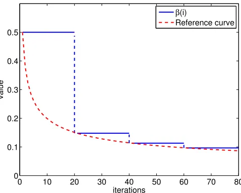
should also decrease drastically prior to steady-state so that the vanishing momentum term will not introduce additional gradient noise and degrade performance. One strategy, which is also employed in the numerical experiments in Section 7, is to design β(i) to decrease in a stair-wise fashion, namely,
β(i) =
β0 ifi∈[1, T], β0/Tα ifi∈[T + 1,2T], β0/(2T)α ifi∈[2T + 1,3T], β0/(3T)α ifi∈[3T + 1,4T],
· · ·
0 10 20 30 40 50 60 70 80 0
0.1 0.2 0.3 0.4 0.5
iterations
value
β(i)
Reference curve
Figure 1: β(i) changes with iteration i according to (84), where β0 = 0.5, T = 20 and α= 0.4. The reference curve isf(i) = 0.5/i0.4.
where the constants β0 ∈ [0,1), α ∈ (0,1) and T > 0 determines the width of the stair steps. Fig. 1 illustrates howβ(i) varies when T = 20, β0 = 0.5 andα= 0.4.
Algorithm (81)–(82) works well when β(i) decreases according to (84) (see Section 7). However, with Theorems 8 and 11, we find that this algorithm is essentially equivalent to the standard stochastic gradient method with decaying step-size, i.e.,
xi =xi−1−µs(i)∇wQ(xi−1;θi), (85)
where
µs(i) = µ
1−β(i) (86)
will decrease from µ/[1−β(0)] to µ. In another words, the stochastic algorithm with decaying momentum is still not helpful.
6. Diagonal Step-size Matrices
Sometimes it is advantageous to employ separate step-size for the individual entries of the weight vectors, see (Duchi et al., 2011). In this section we comment on how the results from the previous sections extend to this scenario. First, we note that recursion (2) can be generalized to the following form, with a diagonal matrix serving as the step-size parameter:
xi =xi−1−D∇wQ(xi−1;θi), i≥0, (87)
the letter “w” for the momentum recursion. We let µmax = max{µ1, . . . , µM}. Similarly, recursions (22) and (23) can be extended in the following manner:
ψi−1 = wi−1+B1(wi−1−wi−2), (88) wi = ψi−1−Dm∇wQ(ψi−1;θi)+B2(ψi−1−ψi−2), (89) with initial conditions
w−2 =ψ−2 = initial states, (90)
w−1 =w−2−Dm∇wQ(w−2;θ−1), (91)
where B1 = diag{β11, . . . , βM1 } and B2 = diag{β12, . . . , βM2 } are momentum coefficient ma-trices, whileDm is a diagonal step-size matrix for momentum stochastic gradient method. In a manner similar to (26), we also assume that
0≤Bk < IM, k = 1,2, B1+B2 =B, B1B2 = 0. (92) where B = diag{β1, . . . , βM} and 0 < B < IM. In addition, we further assume that B is not too close to IM, i.e.
B ≤(1−)IM, for some constant >0. (93)
The following results extend Theorems 1, 3, and 4 and they can be established following similar derivations.
Theorem 1B (Mean-square stability). Let Assumptions 1 and 2 hold and recall con-ditions (92) and (93). Then, for the momentum stochastic gradient method (88)–(89), it holds under sufficiently small step-size µmax that
lim sup i→∞ E
kweik2 =O(µmax). (94)
Theorem 3B (Equivalence for quadratic costs). Consider recursions (52) and (56)–
(57) with {µ, µm, β1, β2} replaced by {D, Dm, B1, B2}. Assume they start from the same
initial states, namely, ψ−2 = w−2 =x−1. Suppose further that conditions (92) and (93)
hold, and that the step-sizes matrices {D, Dm} satisfy a relation similar to (60), namely,
D= (I−B)−1Dm. (95)
Then, it holds under sufficiently small µmax, that
Ekwei−xeik
2 =O(µ2
max), ∀i= 0,1,2,3, . . . (96)
Suppose conditions (92), (93), and (95) hold. Under Assumptions 1, 3, 5, and 6, and for sufficiently small step-sizes, it holds that
Ekwei−xeik
2 =O(µ3/2
max), ∀i= 0,1,2,3, . . . (97)
Furthermore, in the limit,
lim sup i→∞ E
kwei−xeik
2=O(µ2
max). (98)
7. Experimental Results
In this section we illustrate the main conclusions by means of computer simulations for both cases of mean-square-error designs and logistic regression designs. We also run simulations for algorithm (81)–(82) and verify its advantages in the stochastic context.
7.1 Least Mean-Squares Error Designs
We apply the standard LMS algorithm to (47). To do so, we generate data according to the linear regression model (48), wherewo ∈R10 is chosen randomly, and ui ∈R10 is i.i.d
and follows ui ∼ N(0,Λ) where Λ ∈ R10×10 is randomly-generated diagonal matrix with
positive diagonal entries. Besides, v(i) is also i.i.d and follows v(i) ∼ N(0, σs2I10), where σ2
s = 0.01. All results are averaged over 300 random trials. For each trial we generated 800 samples of ui,v(i) andd(i).
0 500 1000 1500 2000 2500 −45
−40 −35 −30 −25 −20 −15 −10 −5 0 5
iterations
MSD(dB)
LMS (52) with µ
Momentum (56)−(57) with µ m=µ
Momentum (56)−(57) with µ m=µ(1−β)
Decaying β(i) (81)−(82) with µm=µ
(85) with µ
s(i) = µ / (1 −β(i))
0 500 1000 1500 2000 2500 −45
−40 −35 −30 −25 −20 −15 −10 −5 0 5
iterations
MSD(dB)
LMS (52) with µ
Momentum (56)−(57) with µ m=µ
Momentum (56)−(57) with µ m=µ(1−β)
Decaying β(i) (81)−(82) with µm=µ
(85) with µ
s(i) = µ / (1 −β(i))
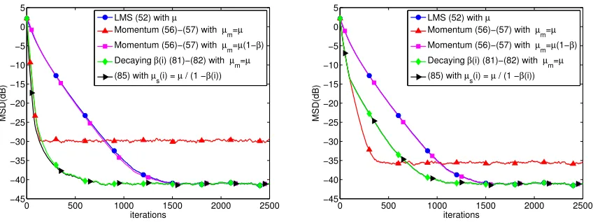
Figure 2: Convergence behavior of standard and momentum LMS (heavy-ball LMS) algo-rithms applied to the mean-square-error design problem (47) with β = 0.9 in the left plot andβ = 0.5 in the right plot. Mean-square-deviation (MSD) means
Ekwo−wik2.
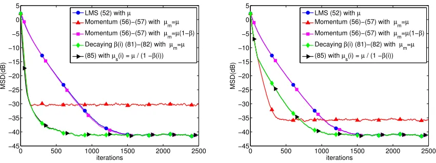
Next we employ the Nesterov’s acceleration option for the momentum LMS method, and compare it with standard LMS. The experimental settings are exactly the same as the above except that β1 = β and β2 = 0. Both the standard and momentum LMS methods are illustrated in Fig. 3. As implied by Theorem 8, it is observed that Nesterov’s acceleration applied to LMS is equivalent to standard LMS with rescaled step-size. Besides, by comparing Figs. 2 and 3, it is also observed that both momentum options, the heavy-ball and the Nesterov’s acceleration, have the same performance. To save space, in the following experiments in Section 7.2–7.4 we just show the performance of momentum method with the option of heavy-ball.
7.2 Regularized Logistic Regression
We next consider a regularized logistic regression risk of the form:
J(w) =∆ ρ 2kwk
2+
E n
ln
1 + exp(−γ(i)hTiw)o
(99)
where the approximate gradient vector is chosen as
∇wQ(w;hi,γ(i)) =ρw−
exp(−γ(i)hTi w)
1 + exp(−γ(i)hTi w)γ(i)hi (100)
In the simulation, we generate 20000 samples (hi,γ(i)). Among these training points, 10000 feature vectors hi correspond to labelγ(i) = 1 and eachhi ∼ N(1.5×110, Rh) for some diagonal covarianceRh. The remaining 10000 feature vectors hi correspond to label
0 500 1000 1500 2000 2500 −45
−40 −35 −30 −25 −20 −15 −10 −5 0 5
iterations
MSD(dB)
LMS (52) with µ
Momentum (56)−(57) with µ m=µ
Momentum (56)−(57) with µ m=µ(1−β)
Decaying β(i) (81)−(82) with µm=µ
(85) with µ
s(i) = µ / (1 −β(i))
0 500 1000 1500 2000 2500 −45
−40 −35 −30 −25 −20 −15 −10 −5 0 5
iterations
MSD(dB)
LMS (52) with µ
Momentum (56)−(57) with µ m=µ
Momentum (56)−(57) with µ m=µ(1−β)
Decaying β(i) (81)−(82) with µm=µ
(85) with µ
s(i) = µ / (1 −β(i))
Figure 3: Convergence behavior of standard and momentum LMS (Nesterov’s acceleration LMS) algorithms applied to the mean-square-error design problem (47) withβ= 0.9 in the left plot andβ = 0.5 in the right plot.
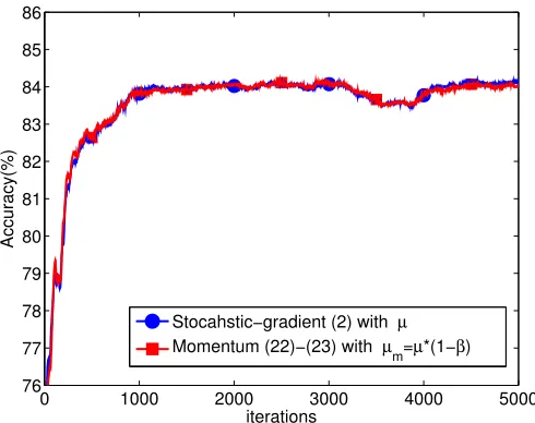
Similar to the least-mean-squares error problem, we first compare the standard and momentum stochastic methods using µ=µm = 0.005. The momentum parameter β is set to 0.9. These two methods are illustrated in Fig. 4 with blue and red curves, respectively. It is seen that the momentum method converges faster, but the MSD performance is much worse. Next we set µm = µ(1−β) = 0.0005 and illustrate this case with the magenta curve. It is observed that the magenta and blue curves are indistinguishable, which confirms the equivalence predicted by Theorem 11 for all time instants. Again we illustrate an implementation with a decaying momentum parameter β(i) by the green curve. In this simulation, we set µm = 0.005 and make β(i) decrease in a stair-wise manner: when i ∈ [1,200], β(i) = 0.9; when i ∈ [201,400], β(i) = 0.9/(2000.3); when i ∈ [401,600], β(i) = 0.9/(4000.3); . . .; when i ∈ [1801,2000], β(i) = 0.9/(18000.3). With this decaying β(i), it is seen that the momentum method recovers its faster convergence rate and attains the same steady-state MSD performance as the stochastic-gradient implementation. Finally, we implemented the standard stochastic gradient descent with initial step-sizeµm =µ= 0.005 and then decrease it gradually according toµs(i) =µ/[1−β(i)]. As implied by Theorem 11, it is observed that the green and black curves are almost indistinguishable, which confirms that the algorithm with decaying momentum is still equivalent to the standard stochastic gradient descent with appropriately chosen decaying step-sizes.
Next, we test the standard and momentum stochastic methods for regularized logistic regression problem over a benchmark data set — the Adult Data Set2. The aim of this dataset is to predict whether a person earns over $50K a year based on census data such as age, workclass, education, race, etc. The set is divided into 6414 training data and 26147 test data, and each feature vector has 123 entries. In the simulation, we setµ= 0.1,ρ= 0.1, and β = 0.9. To check the equivalence of the algorithms, we setµm = (1−β)µ= 0.01. In Fig. 5,
0 500 1000 1500 2000 −18
−16 −14 −12 −10 −8 −6 −4 −2 0 2
iterations
MSD(dB)
Stochastic−gradient (2)
Momentum (22)−(23) with µ
m = µ
Momentum (22)−(23) with µ
m=µ(1−β)
Decaying β(i) (81)−(82) with µ
m = µ Decaying step−size (85)−(86)
Figure 4: Convergence behaviors of standard and momentum stochastic gradient methods applied to the logistic regression problem (99).
the curve shows how the accuracy performance, i.e., the percentage of correct prediction, over the test dataset evolved as the algorithm received more training data3. The horizontal x-axis indicates the number of training data used. It is observed that the momentum and standard stochastic gradient methods cannot be distinguished, which confirms their equivalence when training the Adult Data Set.
For the experiments shown in this section, Section 7.3 and 7.4, we also tested the cases whenβis set as 0.5, 0.6, 0.7, 0.8. Since the experimental results with differentβ are similar, we just plot the situation when β = 0.9, a setting which is usually employed in practice (Szegedy et al., 2015; Krizhevsky et al., 2012; Zhang and LeCun, 2015).
7.3 Further Verification of Theorems 8 and 11
In this section we further illustrate the conclusions of Theorems 8 and 11 by checking the behavior of the iterate difference, i.e.,Ekwi−xik2, between the standard and momentum stochastic gradient methods.
For the least-mean-squares error problem, the selection of ui, v(i), d(i) and β is the same as in the simulation generated earlier in Subsection 7.1. For some specific step-size µ, xi is the iterate generated through LMS recursion (52) with step-size µ, and wi is the iterate generated momentum LMS recursion (56)–(57) with step-sizeµm =µ(1−β). Now we introduce the maximum difference:
dmax(µ) = max
i Ekwi−xik
2 (101)
0 1000 2000 3000 4000 5000 76
77 78 79 80 81 82 83 84 85 86
iterations
Accuracy(%)
Stocahstic−gradient (2) with µ Momentum (22)−(23) with µm=µ*(1−β)
Figure 5: Performance accuracy of the standard and momentum stochastic gradient methods ap-plied to logistic regression classification on the adult data test set.
and the difference at steady state
dss(µ) = lim sup i→∞ E
kwi−xik2. (102) Note that both dmax(µ) and dss(µ) are related with µ and we will examine how they vary according to different step-sizes. Obviously, since Ekwi −xik2 ≤ dmax(µ), if dmax(µ) is illustrated to be on the order ofO(µ2), then it follows that
Ekwi−xik2 =O(µ2) fori≥0. Similarly, if we can illustratedss(µ) =O(µ2), then it follows that lim supi→∞Ekwi−xik2= O(µ2).
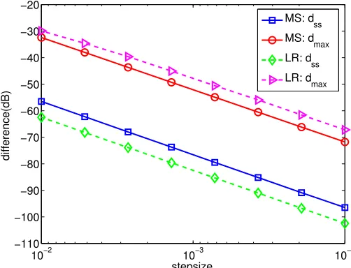
Note that the fact dmax(µ) =cµ2 for some constantcholds if and only if
dmax(µ)(dB) = 20 logµ+ 10 logc, (103) where dmax(µ)(dB) = 10 logdmax(µ). Relation (103) can be confirmed with red circle line in Fig. 6. In this simulation, we choose 8 different step-size values{µk}8k=1, and it can be verified that each data pair
logµk, dmax(µk)(dB)
satisfies relation (103). For example, in
the red circle solid line, atµ1 = 10−2 we read dmax(µ1)(dB) =−32dB; while atµ2 = 10−4 we readdmax(µ2)(dB) =−72dB. It can be verified that
dmax(µ1)(dB)−dmax(µ2)(dB) = 20(logµ1−logµ2) = 40. (104) Using a similar argument, the blue square solid line can also implies thatdss=O(µ2).
Figure 6 also reveals the order of dmax and dss, with magenta and green dash lines respectively, for the regularized logistic regression problem from Subsection 7.2. With the same argument as above,dss(µ) can be confirmed on the order ofO(µ2). Now we check the order ofdmax(µ). The fact thatdmax(µ) =cµ3/2 holds if and only if
According to the above relation, at µ1= 10−2 and µ2 = 10−4 we should have
dmax(µ1)(dB)−dmax(µ2)(dB) = 15(logµ1−logµ2) = 30. (106) However, in the triangle magenta dash line we read dmax(µ1) =−30dB while dmax(µ2) =
−66dB and hence
30dB< dmax(µ1)(dB)−dmax(µ2)(dB)<40dB
Therefore, the order of dmax should be between O(µ3/2) and O(µ2), which still confirms Theorem 11.
10−4
10−3
10−2
−110 −100 −90 −80 −70 −60 −50 −40 −30 −20
stepsize
difference(dB)
MS: dss
MS: d max
LR: dss
LR: dmax
Figure 6: dmax and dss as a function of the step-sizeµ. MS stands for mean-square-error and LR
stands for logistic regression.
7.4 Visual Recognition
In this subsection we illustrate the conclusions of this work by re-examining the problem of training a neural network to recognize objects from images. We employ the CIFAR-10 database4, which is a classical benchmark dataset of images for visual recognition. The CIFAR-10 dataset consists of 60000 color images in 10 classes, each with 32×32 pixels. There are 50000 training images and 10000 test images. Similar to (Sutskever et al., 2013), and since the focus of this paper is on optimization, we only report training errors in our experiment.
To help illustrate that the conclusions also hold for non-differentiable and non-convex problems, in this experiment we train the data with two different neural network struc-tures: (a) a 6-layer fully connected neural network and (b) a 4-layer convolutional neural network, both with ReLU activation functions. For each neural network, we will compare the performance of the momentum and standard stochastic gradient methods.
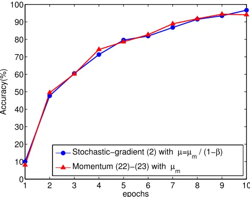
6-Layer Fully Connected Nuerual Network. For this neural network structure, we employ the softmax measure with`2 regularization as a cost objective, and the ReLU as an activation function. Each hidden layer has 100 units, the coefficient of the`2 regularization term is set to 0.001, and the initial valuew−1 is generated by a Gaussian distribution with 0.05 standard deviation. We employ mini-batch stochastic-gradient learning with batch size equal to 100. First, we apply a momentum backpropagation (i.e., momentum stochastic gradient) algorithm to train the 6-layer neural network. The momentum parameter is set to β = 0.9, and the initial step-size µm is set to 0.01. To achieve better accuracy, we follow a common technique (e.g., (Szegedy et al., 2015)) and reduceµm to 0.95µmafter every epoch. With the above settings, we attain an accuracy of about 90% in 80 epochs.
However, what is interesting, and somewhat surprising, is that the same 90% accuracy can also be achieved with the standard backpropagation (i.e., stochastic gradient descent) algorithm in 80 epochs. According to the step-size relation µ = µm/(1−β), we set the initial step-size µ of SGD to 0.1. Similar to the momentum method, we also reduceµ to 0.95µ after every epoch for SGD, and hence the relation µ = µm/(1−β) still holds for each iteration. From Figure 7, we observe that the accuracy performance curves for both scenarios, with and without momentum, are overlapping even when the overall risk is not necessarily convex or differentiable.
0 10 20 30 40 50 60 70 80
0 10 20 30 40 50 60 70 80 90 100
iterations
Accuracy(%)
Stochastic−gradient (2) with µ = µm/ (1−β)
Momentum (22)−(23) with µ
m
Figure 7: Classification accuracy of the standard and momentum stochastic gradient methods ap-plied to a 6-layer fully-connected neural network on the CIFAR-10 test data set.
4-Layer Convolutional Neural Network. In a second experiment, we consider a 4-layer convolutional neural network. We employ the same objective and activation functions. This network has the structure:
conv – ReLU – pool ×2 – affine – ReLU – affine
7×7×32, stride value 1, zero padding 3, and the number of filters is still 32. We implement MAX operation in all pooling layers, and the pooling filters are of size 2×2, stride value 2 and zero padding 0. The hidden layer has 500 units. The coefficient of the`2 regularization term is set to 0.001, and the initial valuew−1 is generated by a Gaussian distribution with 0.001 standard deviation. We employ mini-batch stochastic-gradient learning with batch size equal to 50, and the step-size decreases by 5% after each epoch.
First, we apply the momentum backpropagation algorithm to train the neural network. The momentum parameter is set atβ= 0.9, and we performed experiments with step-sizes µm∈ {0.01,0.005,0.001,0.0005,0.0001}and find thatµm= 0.001 gives the highest training accuracy after 10 epochs. In Fig. 8 we draw the momentum stochastic gradient method with red curve when µm = 0.001 and β = 0.9. The curve reaches an accuracy of 94%. Next we set the step-size of the standard backpropagation µ = µm/(1−β) = 0.01, and illustrate its convergence performance with the blue curve. It is also observed that the two curves are indistinguishable. The numerical results shown in Figs. 7 and 8 imply that the performance of momentum SGD can still be achieved by standard SGD by properly adjusting the step-size according to µ=µm/(1−β).
1 2 3 4 5 6 7 8 9 10
0 10 20 30 40 50 60 70 80 90 100
epochs
Accuracy(%)
Stochastic−gradient (2) with µ=µm / (1−β)
Momentum (22)−(23) with µm
Figure 8: Classification accuracy of the standard and momentum stochastic gradient methods ap-plied to a 4-layer convolutional neural network on the CIFAR-10 training data set.
8. Comparison for Larger Step-sizes
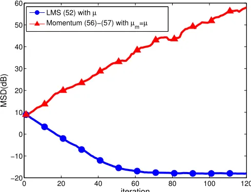
compare to each other under larger step-sizes. For example, it is known that the larger the step-size value is, the more likely it is that the stochastic-gradient algorithm will become unstable. Does the addition of momentum help enlarge the stability range and allow for proper adaptation and learning over a wider range of step-sizes?
Unfortunately, the answer to the above question is generally negative. In fact, we can construct a simple numerical example in which the momentum can hurt the stability range. This example considers the case of quadratic risks, namely problems of the form (47). We suppose M = 5, ui ∼ N(0,0.5I5) and d(i) = uTi wo+v(i) where v(i) ∼ N(0,0.01). We compare the convergence of standard LMS and Nesterov’s acceleration method with fixed parameter β2 = 0 and β = 0.5. Both algorithms are set with the same step-size µ = µm = 0.4, which is a relatively large step-size. All results are averaged over 1000 random trials. For each trial we generated 200 samples of ui, v(i) and d(i). In Fig. 9, it shows that standard LMS converges at µ = 0.4 while momentum LMS diverges, which indicates that momentum LMS has narrower stability range than standard LMS.
0 20 40 60 80 100 120
−20 −10 0 10 20 30 40 50 60
iteration
MSD(dB)
LMS (52) with µ
Momentum (56)−(57) with µ
m=µ
Figure 9: Convergence comparison between standard and momentum LMS algorithms when µ=µm = 0.4 andβ = 0.5.
9. Conclusion
to the stochastic setting when adaptation becomes necessary and gradient noise is present. The analysis also comments on a way to retain some of the advantages of the momentum construction by employing a decaying momentum parameter: one that starts at a con-stant level and decays to zero over time. adaptation is retained without the often-observed degradation in MSD performance.
Acknowledgments
This work was supported in part by NSF grants CIF-1524250 and ECCS-1407712, by DARPA project N66001-14-2-4029, and by a Visiting Professorship from the Leverhulme Trust, United Kingdom. The authors would like to thank PhD student Chung-Kai Yu for contributing to Section 5.3, and undergraduate student Gabrielle Robertson for contributing to the simulation in Section 7.4.
Appendix A. Proof of Lemma 2
It is shown in Eq. (3.76) of (Sayed, 2014a) that Ekweik
4 evolves as follows:
Ekweik
4 ≤(1−µν)
Ekwei−1k
4+a
1µ2Ekwei−1k
2+a
2µ4, (107) where the constantsa1 and a2 are defined as
a1 ∆
= 16σ2s, a2 ∆
= 3σs,44 . (108) If we iterate (16) we find that
Ekweik
2 ≤(1−µν)i+1
Ekwe−1k
2+a
3µ, (109)
wherea3 is defined as
a3 ∆ = σ
2 s
ν . (110)
Substituting inequality (109) into (107), we find that it holds for each iterationi= 0,1,2, . . .
Ekweik
4≤(1−µν)
Ekwei−1k
4+a
2µ4+a1a3µ3+a4µ2(1−µν)i, =ρEkwei−1k
4+a
2µ4+a1a3µ3+a4µ2ρi (111) where
ρ = 1∆ −µν, a4 ∆
= a1Ekwe−1k
2. (112)
Iterating the inequality (111) we get
Ekweik
4 ≤ρi+1
Ekwe−1k
4+a 2µ4
i
X
s=0
ρs+a1a3µ3 i
X
s=0
ρs+a4µ2(i+ 1)ρi
≤ρi+1Ekwe−1k
4+a2µ4 1−ρ +
a1a3µ3 1−ρ +a4µ