Variable Selection Using SVM based Criteria     (Kernel Machines Section)

Variable Selection Using SVM-based Criteria

Alain Rakotomamonjy [email protected]

Perception, Syst`emes et Information FRE CNRS 2645

INSA de Rouen

76801 Saint Etienne du Rouvray France

Editors: Isabelle Guyon and Andr´e Elisseeff

Abstract

We propose new methods to evaluate variable subset relevance with a view to variable selection. Relevance criteria are derived from Support Vector Machines and are based on weight vector

kwk2_{or generalization error bounds sensitivity with respect to a variable. Experiments on linear} and non-linear toy problems and real-world datasets have been carried out to assess the effective-ness of these criteria. Results show that the criterion based on weight vector derivative achieves good results and performs consistently well over the datasets we used.

Keywords: support vector machines, kernels, variable selection, sensitivity.

1. Introduction

Nowadays, many practical pattern recognition tasks infer knowledge from example data. This knowledge is then used to make predictions about new data or to get a deeper understanding of the system or “concept” that generated the data. Data typically consist of measurements (also referred to as attributes, variables or features) characterizing the system to be modelled. Each example may be represented as a vector inRnwhose components correspond to such measurements. In a pattern recognition or discrimination problems each example vector is associated with a label specifying the category the example belongs to. Machine learning algorithms estimate dependencies between the examples and their label during a learning process. Progresses made in sensor technology and data management allow researchers to gather data sets of ever increasing sizes, particularly with respect to the number of variables. However, the incremental informative content of such variables is not always significant. This problem may undermine the success of machine learning that is strongly affected by data quality: redundant, noisy or unreliable information may impair the learning process.

The purpose of feature or variable selection is to eliminate irrelevant variables to enhance the generalization performance of a given learning algorithm. The selection of relevant variables may also be useful to gain some insight about the concept to be learned. Other advantages of feature selection include cost reduction of data gathering and storage (in medical applications for instance) and computational speedup.

an extension of the SVM-RFE algorithm (Guyon et al., 2000). Extensive experiments are con-ducted to compare various methods. The paper is organized as follows: In Section 2 we review SVMs and give details on how variable relevance criteria are derived from the SVM methodol-ogy. The associated variable selection algorithm is then presented. Numerical experiments on toy problems and real-world data showing the strength and weakness of different criteria are de-scribed in Section 3. Discussions about the questions that have arisen from this work are reported in Section 4.

2. Variable Selection with SVM Criterion

In this section, we explore some possible methods of variable selection using support vector machines. After reviewing the so-called soft margin SVM classifier, we present ranking criteria derived from SVM and an associated algorithm for feature selection. Finally, relationships with other SVM-based feature selection methods are given.

2.1 SVM Classifier

The support vector machine classifier is a binary classifier algorithm that looks for an optimal hyperplane as a decision function in a high-dimensional space (Boser et al., 1992, Vapnik, 1998, Cristianini and Shawe-Taylor, 2000). Consider one has a training data set{xk,yk} ∈Rn× {−1,1}

where xkare the training examples and yk the class labels. The method consists in first mapping x

into a high dimensional space via a functionΦ, then computing a decision function of the form:

f(x) =hw,Φ(x)i+b

by maximizing the distance between the set of pointsΦ(xk)to the hyperplane parameterized by

(w,b)while being consistent on the training set. The class label of x is obtained by considering the sign of f(x). For the SVM classifier with misclassified examples being quadratically penalized, this optimization problem can be written as:

min

w,ξ

1 2kwk

2_+C

∑

m

k=1 ξ2

k

under the constraint∀k, ykf(xk)≥1−ξk. The solution of this problem is obtained using the

Lagrangian theory and one can prove that vector w is of the form:

w=

m

∑

k=1

α∗

kykΦ(xk)

whereα∗_k is the solution of the following quadratic optimization problem:

max

α W(α) =

m

∑

k=1

αk−

1 2

m

∑

k,`

αkα`yky`

K(xk,x`) +

1

Cδk,`

(4)

The interesting point of SVMs is that they are provided with many statistics that allow to estimate their generalization performance from bounds on the leave-one-out error

L

. The leave-one-out error is the number of classification error produced by the leave-leave-one-out procedure which consists in learning a decision function from m−1 examples, testing the remaining one and re-peating until all elements have served as test example. The leave-one-out error is known to be an unbiased estimator of the generalization performance of a classifier trained on m−1 exam-ples. One of the most common

L

error bounds for SVMs is the radius/margin bound (for decision function with non-zero bias b) (Vapnik, 1998):

L

≤4R2kwk2

where R is the radius of the smallest sphere that contains all the mapped dataΦ(xk). A tighter

bound named “span estimate” is also available and is based on the distance Spbetween a mapped

support vectorΦ(xp)and the span of all other support vectors (Vapnik and Chapelle, 2000). The

following equation holds:

L

≤

∑

p

α∗

pS2p

where S2_p, for SVM with quadratic slack variables ξ, is related to the extended matrix of the dot product between support vectors

∼ KSV=

K 1

1T 0

by the equation S2_p=1/(K∼− 1

SV)pp

2.2 SVM-RFE Algorithm

The SVM-RFE algorithm has been recently proposed by Guyon et al. (2000) for selecting genes that are relevant for a cancer classification problem. The goal is to find a subset of size

r among d variables (r<d) which maximizes the performance of the predictor. The method is

based on a backward sequential selection. One starts with all the features and removes one feature at a time (in their paper, due to the large amount of genes, they remove chunks of features) until r features are left. The removed variable is the one whose removal minimizes the variation ofkwk2. Hence, the ranking criterion Rcfor a given variable i is:

kwk2− kw(i)k2=1

2

∑

_k,jα∗kα∗jykyjK(xk,xj)−

∑

k,j

α∗(i)

k α

∗(i)

j ykyjK(i)(xk,xj)

(8)

where K(i)is the Gram matrix of the training data when variable i is removed (K_k(i_,)_j=hΦ(x_k(i)),Φ(x(_ji))i)

2.3 Algorithm for Variable Ranking with SVM

Variable selection algorithms require a ranking criterion to rank variables. In many papers, bounds on the

L

error have been used for model selection (Duan et al., 2002) and recently We-ston et al. (2001b) used the radius/margin bound for feature selection using a gradient descent algorithm. This idea can therefore be extended to other bounds of the generalization error. In this paper, we will investigate three criteria Ct which are either the weight vectorkwk2, the

ra-dius/margin bound R2kwk2 or the span estimate. These criteria give either an estimation of the generalization performance (the bounds) or an estimation of the dataset separability. Furthermore, similarly to neural-networks based variable selection (Leray and Gallinari, 1999), two approaches can be proposed for each criterion:

• Zero-order method: in this case, the criterion Ct is directly used for variable ranking, and

the methods consists in identifying the variable that produces the smallest value of Ct when

removed. The ranking criterion then becomes Rc(i) =Ct(i)with C( i)

t being the criterion value

when variable i has been removed.

• First-order method: one uses the derivatives of the criterion Ct with regards to a variable. In

other words, this approach differs from the previous one since a variable is ranked according to its influence on the criterion which is measured with the absolute value of the derivative. In this case, the ranking criterion is Rc(i) =|∇Ct|.

The zero-order criteria based on bounds have already been used for feature selection associated with different search space algorithm (Weston et al., 2001b) whereas the first-order ones are rather new for the purpose of feature selection.

Similarly to SVM-RFE, the problem of searching the “best” r variables is solved by means of a greedy algorithm based on backward selection (Kohavi and John, 1997). A backward sequential selection is used because of its lower computational complexity compared to randomized or expo-nential algorithms and its optimality in the subset selection problem (Couvreur and Bresler, 2000). Hence, the algorithm starts with all features and repeatedly removes a feature until r features are left or all variables have been ranked (see Figure 1). In the zero-order method, one suppresses the feature whose removal minimizes the criterion whereas in first-order methods, one removes the variable to which the criterion is less sensitive. For instance, in the zero-orderkwk2 case, the ranking term is:

Rc(i) =kw(i)k2=

∑

k,j

α∗(i)

k α

∗(i)

j ykyjK(i)(xk,xj) (9)

where K(i)is again the Gram matrix of the training data when the variable i has been removed. Note that in this case, the criterion should be evaluated with the appropriate α∗_k(i). Similarly to SVM-RFE and to reduce time complexity we consider that these parameters are equal toα∗_k during the evaluation of Rc(i). However, it would still be interesting to consider how the SVM

retraining at each subset evaluation affects the results and some experiments using the trueα∗_k(i) will be carried out.

In the first-order case, the ranking term forkwk2case criterion would be:

1. Initialization: Ranked= []; Var= [1,...,N]

2. repeat

(a) Train a SVM classifier with all the training data and the variables Var

(b) for all variables in Var, do evaluate the ranking criterion Rc(i)of variable i endfor

(c) best=arg miniRc

(d) rank the variable that minimizes Rc: Ranked= [best Ranked];

(e) remove the variable that minimizes Rc from the selected variables set: Var =

[1,...,best−1,best+1,...,N]

3. until Var is not empty

Figure 1: Outline of the SVM-based feature selection algorithm.

2.4 Calculating the Gradient with Regards to a Scaling Factorν

For the first-order criterion, our aim is to measure the sensitivity of a given criterion with respect to a variable. A possible approach is to introduce a virtual scaling factor and to compute the gradient of a criterion with respect to that scaling factorν. The latter acts as a componentwise multiplicative term (whose value is 1) on the input variables and thus k(x,x0)becomes:

k(ν·x,ν·x0)

where · denotes the componentwise vector product. Consequently, one obtains the following

derivatives for a Gaussian Kernel k(ν·x,ν·x0) =e−k

ν·x−ν·x0k2

2σ2 :

∂k ∂νi =−

1

σ2(νixi−νix

0

i)2k(x,x0) =−

1

σ2(xi−x

0

i)2k(x,x0)

where we used the fact thatνi=1. Then, one needs to evaluate the gradient of the bounds with

regards to a variableνiand for a given criterion Ct the ranking term becomes :

Rc(i) =

∂Ct(α,b)

∂νi

(11)

where Ct is either kwk2, R2w2or∑pα∗pS2p and depends on the solution of Equation (4) and the

bias b. Details of the derivatives computation for a given criterion are presented in the report of Rakotomamonjy (2002), and they have been obtained using the results of Bengio (2000) and Chapelle et al. (2002). Here, we only give the final results:

• weight vector gradient:

Rc(i) =

∑

_k,jα∗kα∗jykyj

∂k(ν·xk,ν·xj)

∂νi

• radius/margin gradient:

Rc(i) =

kwk2

∑

_k,j(βkβj−βkδk,j)

∂k(ν·xk,ν·xj)

∂νi +

R2

∑

k,j

α∗

kα∗jykyj

∂k(ν·xk,ν·xj)

∂νi

where R2is the optimal objective function of the following problem: max_β ∑_kβkk(ν·xk,ν·xk)−∑k,jβkβjk(ν·xk,ν·xj)

s.t ∑_kβk and βk≥0∀k

• span estimate gradient:

Rc(i) =

`

∑

p=1

2

−H−1∂H

∂νi

α∗

pp

S2_p+α∗_pS4_p K∼− 1

SV

∂K∼SV

∂νi

∼ K−

1

SV

!

pp

where H is the following matrix H=

KY Y YT 0

and KY_{k j}=ykyjk(ν·xk,ν·xj)

As noticed previously all these gradients are computed forν= (1,..,1). In what follows, we use the notation∇Ct to denote these first order criteria where Ct is eitherkwk2, R2w2or∑pα∗pS2p.

2.5 Relation to Other SVM-Based Feature Selection Methods

In addition to SVM-RFE, several algorithms for feature selection based on SVM are already available. For instance, Weston et al. (2001b) propose a method based on finding the best variable subset which minimizes the R2w2bound. For this criterion, their method differs from ours in the variable space search algorithm. In fact instead of using a greedy algorithm, they use a gradient descent to minimize the bound with respect to a scaling vector associated to variables.

In the linear case, an interesting relation links SVM-RFE and our method when using the derivatives ofkwk2 _{with respect to a virtual scaling factor. The RFE criterion for a variable i is} Rc(i) =w2i whereas the gradient of kwk2 with respect to νi gives Rc(i) =| −w2i|(νi being the

scaling factor associated to variable i). Thus, SVM-RFE and gradient ofkwk2are identical as they have the same ranking criterion.

In addition, one should note that SVM-RFE and the zero-order kwk2 criterion are identical since the first sum in Equation (8) is constant during the evaluation of Rc(i). For this reason,

results concerning SVM-RFE are not reported in the experimental section.

3. Numerical Experiments

The experiments that we report here use artificial and real-world datasets. We have compared the classification performance of the different ranking criteria for feature selection associated to a SVM classifier with quadratic slack variablesξias a predictor. In addition, in all experiments the

Training set size

Methods 10 20 30 40 50

SVM 36.58%±2% 30.89%±2% 25.46%±2% 22.22%±2 % 19.40%±2% Corr 32.33%±13% 17.00%±7% 14.30%±4% 14.69%±2 % 14.76%±2% kwk2 _{35.63%±15% 14.79%±13% 5.99%±5% 4.40%±3% 4.19%±3%} R2_w2 _{32.83%±15% 13.60%±12% 5.82%±5% 4.53%±3% 4.04%±2%} S2

pEst. 38.92%±13% 21.14%±15% 14.22%±12% 10.68%±9% 7.34%±6%

kwik2 32.39%±15% 13.05%±11% 7.14%±6% 6.30%±5% 5.11%±4%

R2

iw2i 31.21%±15% 19.13%±12% 14.55%±9% 14.10%±9% 13.13%±9%

S2

piEst. 50.02%±0.5% 50.02%±0.5% 49.44%±2% 49.83%±2% 49.49%±2%

∇kwk2 _{32.39%±15% 13.05%±11% 7.14%±6% 6.30%±5% 5.11%±4%}

∇R2_w2 _{33.50%±15% 36.87%±16% 43.69%±17% 46.28%±10% 46.81%±9%}

∇S2

pEst 41.51%±12% 23.85%±13% 15.91%±10% 13.76%±9% 13.16%±7%

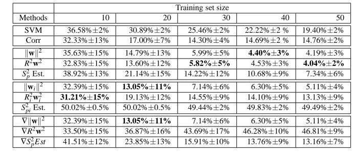
Table 1: Mean and standard deviation of test error for feature selection on a synthetic linear prob-lem using different criteria and different training set sizes. The methods are: (a) SVM: standard SVM,(b) Corr: SVM with correlation coefficients feature selection algorithm, (c) kwk2, R2w2 and S2_p Est zero-order criterion with retraining, (d) kwik2, R2iw2i and

S2_pi Est zero-order criterion. (e)∇kwk2,∇R2w2and∇S2_pEst first-order criterion.

3.1 Toy Experiments

For toy experiments, we used the datasets described in the work of Weston et al. (2001a,b), which allows comparing the results obtained with our criteria to those described in these refer-ences. A precise description of these synthetic data can be found in Weston et al. (2001b). In the 2-class linear problem, the input data are composed of 202 variables from which only 6 are rele-vant whereas, in the nonlinear one, 52 variables are available and only the first two are relerele-vant. In both cases, 10000 points have been generated. Only a randomly-chosen small proportion of them are used as a training set and the rest are included in a test set. The training set has been normalized to get zero mean and unit standard deviation. The test set is normalized according to the training set normalization parameters.

For both feature selection and classification, we used a linear SVM for the linear problem and a Gaussian kernel withσ=3 for the nonlinear problem. In both linear and non-linear cases, the hyperparameter C has been set sufficiently high (respectively C=100000 and C=1000) in order to keep training error low. After feature selection has been performed, only the two top-ranked variables are provided to the predictor.

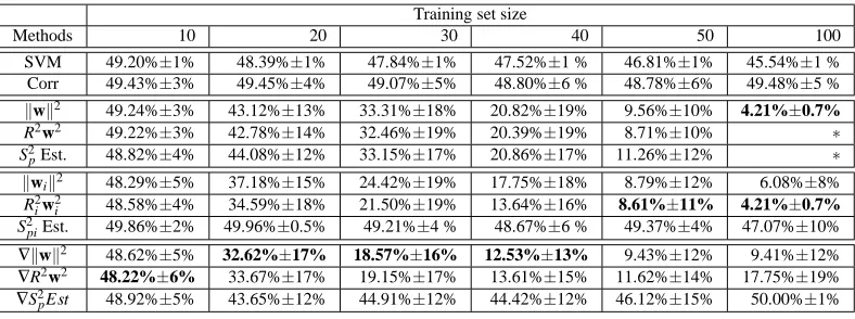
Table 1 and Table 2 present the mean and the standard deviation of the test error over 100 trials for each training set size. For both datasets, SVM without feature selection overfits. When considering the baseline feature selection method based on correlation coefficients, the test error becomes significantly lower in the linear case but does not decrease in the nonlinear problem. This is simply due to the incapability of this feature selection method to represent variable correlation in a nonlinear context.

Training set size

Methods 10 20 30 40 50 100

SVM 49.20%±1% 48.39%±1% 47.84%±1% 47.52%±1 % 46.81%±1% 45.54%±1 % Corr 49.43%±3% 49.45%±4% 49.07%±5% 48.80%±6 % 48.78%±6% 49.48%±5 % kwk2 _{49.24%±3% 43.12%±13% 33.31%±18% 20.82%±19% 9.56%±10% 4.21%±0.7%} R2_w2 _{49.22%±3% 42.78%±14% 32.46%±19% 20.39%±19% 8.71%±10% ∗} S2

pEst. 48.82%±4% 44.08%±12% 33.15%±17% 20.86%±17% 11.26%±12% ∗

kwik2 48.29%±5% 37.18%±15% 24.42%±19% 17.75%±18% 8.79%±12% 6.08%±8%

R2

iw2i 48.58%±4% 34.59%±18% 21.50%±19% 13.64%±16% 8.61%±11% 4.21%±0.7%

S2

piEst. 49.86%±2% 49.96%±0.5% 49.21%±4 % 48.67%±6 % 49.37%±4% 47.07%±10%

∇kwk2 _{48.62%±5% 32.62%±17% 18.57%±16% 12.53%±13% 9.43%±12% 9.41%±12%}

∇R2_w2 _{48.22%±6% 33.67%±17% 19.15%±17% 13.61%±15% 11.62%±14% 17.75%±19%}

∇S2

pEst 48.92%±5% 43.65%±12% 44.91%±12% 44.42%±12% 46.12%±15% 50.00%±1% Table 2: Mean and standard deviation of test error for feature selection on a synthetic non linear

problem using different criteria and different training set sizes. The methods are: (a) SVM: standard SVM,(b) Corr: SVM with correlation coefficients feature selection algo-rithm, (c) kwk2, R2w2 and S2_pEst zero-order criterion with retraining, (d)kwik2, R2iw2i

and S2_piEst zero-order criterion, (e)∇kwk2,∇R2w2and∇S2_pEst first-order criterion. An

asterisk ∗indicates that full experiments had not been carried out because of excessive time.

retraining is performed. The span estimate criterion does well only with retraining. This is merely explained by the tight relation of this span estimate with the value ofα∗ (Vapnik and Chapelle, 2000) and thus keeping α∗ fixed during the evaluation of Rc(i) leads to a wrong estimation of

variable relevance.

Without retraining, in the linear case the ∇kwk2 (which is identical to thekwk2 criterion) outperforms other methods. For the nonlinear problem,∇kwk2 and R2w2 criteria share the best performance depending on the size of the training set.

3.2 Real-World Data

In order to assess the effectiveness of the proposed criteria, experiments on real-world datasets have also been performed.

3.2.1 BENCHMARKDATASETS

1 2 3 4 5 6 7 8 9 0.24

0.25 0.26 0.27 0.28 0.29 0.3 0.31

Zero−Order Criteria

Nb of ranked features

Test error

w2 R2w2 Span Est

1 2 3 4 5 6 7 8 9

0.24 0.25 0.26 0.27 0.28 0.29 0.3 0.31

First−Order Criteria

Nb of ranked features

Test error

Grad w2 Grad R2w2 Grad Span Est

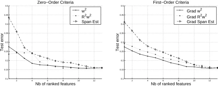
Figure 2: Mean of test error for a feature selection problem on a real-world problem. Mean test er-rors for Breast Cancer Data vs. the number of ranked variables used for training (C=15,

σ=5). (left)kwik2, R2iw2i and S2piEst zero-order criterion. (right)∇kwk2,∇R2w2 and

∇S2_pEst.

2 4 6 8 10 12

0.1 0.15 0.2 0.25 0.3 0.35 0.4 0.45 0.5

Zero−Order Criteria

Nb of ranked features

Test error

w2 R2w2 Span Est

2 4 6 8 10 12

0.1 0.15 0.2 0.25 0.3 0.35 0.4 0.45 0.5

First−Order Criteria

Nb of ranked features

Test error

Grad w2 Grad R2w2 Grad Span Est

Figure 3: Mean of test error of feature selection on real-world problem. Mean test error for Heart Data vs. to the number of ranked variables used for training (C=3.16, σ=7.7) (left)

kwik2, R2iw2i and S2piEst zero-order criterion. (right)∇kwk2,∇R2w2and∇S2pEst.

Number of variables

Methods 20 50 100 250 500 1000

Corr 21.58%±11% 22.08%±10% 20.83%±11% 17.83%±9 % 18.42%±9% 16.75%±9%

R2

iw2i 19.67%±11% 17.33%±9% 16.17%±9% 16.66%±9% 16.53%±8% 15.91%±8%

S2

piEst. 22.66%±12% 34.25%±14% 30.50%±12% 23.83%±10% 18.91%±9% 17.67%±9%

∇w2 _{17.67%±9% 15.66%±9% 15.17%±10% 16.50%±9% 16.08%±9% 16.25%±9%}

∇R2_w2 _{20.33%±13% 17.83%±10% 16.41%±9% 15.58%±9% 16.16%±9% 16.16%±8%}

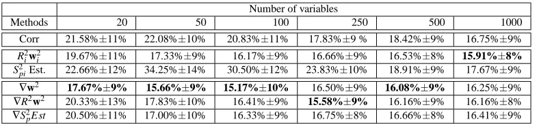
∇S2pEst 20.50%±11% 17.00%±10% 16.33%±9% 16.75%±8% 16.66%±8% 16.41%±9% Table 3: Mean and standard deviation of test error for a feature selection problem on a microarray

Colon Cancer Dataset. The methods are: (a) Corr: SVM with correlation coefficients feature selection algorithm, (b) R2_iw2_i and S2_piEst zero-order criterion, (c)∇kwk2,∇R2w2

and∇S2pEst first-order criterion.

3.2.2 MICROARRAYDATA

Experiments on DNA microarray analysis have also been performed. The data we used con-cerned two classification problems, the first one dealing with normal and cancerous colon tissue and the second one with a lymphoma problem. These datasets have already been used for bench-marking feature selection algorithms (for example, see Weston et al., 2001a).

The colon cancer tissue problem is composed of 62 observations (22 normal and 40 cancerous) described by 2046 features. Following the step of Weston et al. (2001a), the training set and the test set are obtained by splitting the dataset into two groups of respectively 50 and 22 elements, while ensuring that the proportions of positive and negative classes are similar in both sets. 100 trials are carried out with random splitting of dataset. In order to speed up the feature selection procedure, half of the variables are removed at each step until 100 variables remain still to be ranked. Then variables are removed one at a time. The predictor is a linear SVM (with C=106) and it achieves an average test error of 16.4%±8%. Results with an increasing number of features provided to the predictor are described in Table 3. The performances are in the same range but one can see that the criterion ∇kwk2 slightly outperforms the others. Again, retraining does not improve all that much the ability of ranking relevant variables for any of the zero-order criteria.

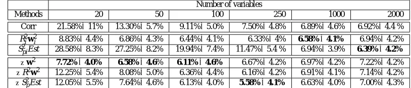
The lymphoma problem is based on 4026 variables describing 96 observations (62 and 34 of which are respectively considered as abnormal and normal). The data is split into two sets of sizes 60 and 36 with similar proportions of abnormal and normal examples. The same methodology as in the colon cancer problem is followed and a linear SVM (with C=106) gives a test error of 7.25%±4.1%. Results obtained with a different number of features and criteria for feature selection are given in Table 4. It seems that the ∇S2_p Est criterion performs better than other

criteria and achieves the best performance with 5.58% test error with only 250 variables. However, it should be noted that with the∇kwk2criterion good performance can be achieved using only 20 variables.

4. Discussions

Number of variables

Methods 20 50 100 250 1000 2000

Corr 21.58%±11% 13.30%±5.7% 9.11%±5.0% 7.50%±4.8% 6.89%±4.6% 6.92%±4.4 %

R2

iw2i 8.83%±4.4% 6.86%±4.3% 6.44%±4.1% 6.33%±4% 6.58%±4.1% 6.94%±4.2%

S2

piEst 28.58%±8.3% 27.25%±8.2% 19.94%±7.4% 11.47%±5.4 % 6.94%±3.9% 6.39%±4.2%

∇w2 _{7.72%±4.0% 6.58%±4.6% 6.11%±4.6% 6.67%±4.2% 6.97%±4.2% 7.22%±4.2%}

∇R2_w2 _{12.25%±5.4% 8.08%±5.0% 6.36%±4.4% 6.16%±4.2% 6.91%±4.1% 7.14%±4.2%}

∇S2pEst 12.05%±5.5% 7.64%±4.6% 6.13%±4.0% 5.58%±4.1% 6.63%±4.0% 7.00%±4.3% Table 4: Mean and standard deviation of test error for a feature selection problem on a microarray

Lymphoma MicroArray Dataset. The methods are: (a) Corr: SVM with correlation coefficients feature selection algorithm, (b) R2_iw2_i and S2_piEst zero-order criterion, (c) ∇kwk2,∇R2w2and∇S2pEst first-order criterion with respect to a scaling factor.

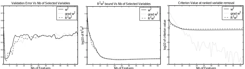
4.1 How Many Ranked Features Must be Used?

Up to now, the question of how many ranked features must be provided to the predictor has not been addressed. Our aim is not to investigate this point completely but rather to suggest some possible solutions.

• The most straightforward idea is to use a leave-one-out procedure or a validation set to esti-mate the generalization error with regards to the number of features and choose the number of variables which minimizes the test error. However, this method is computationally ex-pensive.

• Another approach is to use one of the SVM upper bound of the

L

error (for instance, R2w2) for selecting the best model. The drawback is that these bounds are usually loose bounds and they do not always reflect the generalization performance behavior.

• A classical approach already described in feature selection literature for backward elim-ination is to stop removing variables when the ranking term increases significantly as a variable is removed. Typically, one measures the ranking term Rc(i)and keeps on

eliminat-ing variables as long as Rc(i)is below a threshold. For instance, this means that when using

first-order criterion one can keep on removing variables as long as the derivative norm is below a given threshold.

5 10 15 20 25 30 35 40 45 50 0

0.1 0.2 0.3 0.4 0.5 0.6 0.7 0.8

Validation Error Vs Nb of Selected Variables

Nb of Features

Validation Error

w2 grad w2 R2w2

5 10 15 20 25 30 35 40 45 50 4

4.5 5 5.5 6 6.5 7 7.5 8

R2w2 bound Vs Nb of Selected Variables

Nb of Features

log10 of R

2w

2

w2 grad w2 R2_w2

5 10 15 20 25 30 35 40 45 50 −8

−6 −4 −2 0 2 4 6 8

Criterion Value at ranked variable removal

Nb of Features

log10 of criterion value

w2 grad w2 R2_w2

Figure 4: Different ways of choosing the number of ranked features to be provided to the predic-tor. Results forkwk2,∇kwk2and R2w2are depicted. (left) Validation error. (middle)

L

error Estimation with _m1R2w2. (right) Criterion value when variable has been removed.

4.2 Influence of SVM Hyperparameters

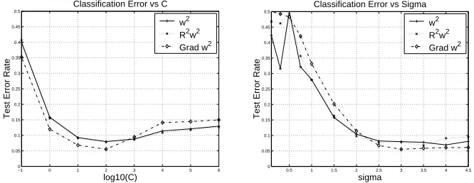
SVMs involve several hyperparameters (e.g. Gaussian kernel parameterσ, degree d of a poly-nomial kernel, slack variables penalization C ) that have to be tuned to achieve the best general-ization performance. This is a crucial issue that is usually solved by minimizing a validation error, a leave-one-out error or an upper bound on the generalization error (Duan et al., 2002, Chapelle et al., 2002, Bengio, 2000). In our feature selection algorithm, these hyperparameters play an important role as they are related to a criterion value through Equation (4). An example of the influence of these hyperparameters on the test error is depicted in Figure 5. The plots represent the mean test error of the nonlinear toy problem using 3 different criteria. The settings are the same as in the experiment involving this data but only C orσis varying over a range of values. These figures clearly show that the problem of model selection is a crucial issue that must be addressed accurately. This point is beyond the scope of this paper but the most intuitive way of solving this problem is by minimizing a validation error. However, this model selection phase can be compu-tationally very expensive since it involves the SVM hyperparameters as well as the choice of the number of features to be used as stated in the previous section.

5. Conclusion

−1 0 1 2 3 4 5 6 0

0.05 0.1 0.15 0.2 0.25 0.3 0.35 0.4 0.45 0.5

log10(C)

Test Error Rate

Classification Error vs C

w2

R2w2

Grad w2

0.5 1 1.5 2 2.5 3 3.5 4 4.5

0 0.05 0.1 0.15 0.2 0.25 0.3 0.35 0.4 0.45 0.5

sigma

Test Error Rate

Classification Error vs Sigma

w2

R2w2

Grad w2

Figure 5: Plots of the influence of C and σ on the test error (averaged over 100 realizations) using the nonlinear toy dataset (training set size is 50). (left) Feature selection and classification error with σ=3 vs C. (right) Feature selection and classification error with C=100 vsσ.

• The ∇kwk2 criterion performs consistently well over all the datasets we used. In addition, it implements a criterion similar to the SVM-RFE criterion in the sense that SVM-RFE measures the sensitivity ofkwk2 to a variable by computing the change inkwk2 when this given variable has been removed. In the linear case, these two methods become identical. Lastly, as it has the lowest time complexity (Rakotomamonjy, 2002), it may be the most useful one for practical applications.

• When a large number of training examples is available, retraining significantly improves the ability of zero-order criterion to select relevant variables at the expense of increased time complexity. Surprisingly, retraining does not always improve the ability of SVMs to select these relevant variables regardless of the criterion used. In cases in which the training set size is small, using the exact α∗(i) in the processing of the ranking term Rc(i) tends to

decrease the performance. Intuitively, one may justify this behavior by the overfitting effects occurring due to the small number of data and the large number of variables. However, this point is far from being clear and some further analysis is needed in order to fully understand this issue.

Examples on real-world data demonstrate the usefulness of the proposed criteria. The perfor-mance obtained without variable selection is either closely matched or improved using far fewer variables selected with the proposed algorithms.

Acknowledgements

The author would like to thank the referees and the editors of this issue for their comments and suggestions, and Jason Weston for making the datasets he used publicly available.

References

Y. Bengio. Gradient-based optimization of hyperparameters. Neural Computation, 12:1889–1900, 2000.

B. E. Boser, I. M. Guyon, and V. N. Vapnik. A training algorithm for optimal margin classifiers. In D. Haussler, editor, 5th Annual ACM Workshop on COLT, pages 144–152, Pittsburgh, PA, 1992. ACM Press.

O. Chapelle, V. Vapnik, O. Bousquet, and S. Mukerjhee. Choosing multiple parameters for svm.

Machine Learning, 46(1-3):131–159, 2002.

C. Couvreur and Y. Bresler. On the optimality of the backward greedy algorithm for the subset selection problem. SIAM Journal on Matrix Analysis and Applications, 21(3):797–808, 2000.

N. Cristianini and J. Shawe-Taylor. Introduction to Support Vector Machines. Cambridge Uni-veristy Press, 2000.

K. Duan, S.S. Keerthi, and A.N. Poo. Evaluation of simple performance measures for tuning svm hyperparameters. Neurocomputing, To appear, 2002.

I. Guyon, J. Weston, S. Barnhill, and V. Vapnik. Gene selection for cancer classification using support vector machines. Machine Learning, 2000.

R. Kohavi and G. John. Wrappers for feature subset selection. Artificial Intelligence, (97):273– 324, 1997.

P. Leray and P. Gallinari. Feature selection with neural networks. Behaviormetrika, 26(1):145– 166, 1999.

A. Rakotomamonjy. Variable selection using svm based criteria. Technical Report 02-004, Insa de Rouen Perception Syst`eme Informations, http://asi.insa-rouen.fr/˜arakotom, 2002.

G. R¨atsch, T. Onoda, and K-R M¨uller. Soft margins for AdaBoost. Machine Learning, 42(3): 287–320, 2001.

V. Vapnik. Statistical Learning Theory. Wiley, 1998.

V. Vapnik and O. Chapelle. Bounds on error expectation for support vector machines. Neural

Computation, 12(9), 2000.

J. Weston, A. Elisseeff, and B. Scholkopf. Use of the `0-norm with linear models and kernel methods. Technical report, BIOwulf Technical Report, 2001a.