Optimality of Graphlet Screening in High Dimensional
Variable Selection
Jiashun Jin [email protected]
Department of Statistics Carnegie Mellon University Pittsburgh, PA 15213, USA
Cun-Hui Zhang [email protected]
Department of Statistics Rutgers University
Piscataway, NJ 08854, USA
Qi Zhang [email protected]
Department of Biostatistics&Medical Informatics University of Wisconsin-Madison
Madison, WI 53705, USA
Editor:Bin Yu
Abstract
Consider a linear modelY =Xβ+σz, whereXhasnrows andpcolumns andz∼N(0, In).
We assume bothpandnare large, including the case ofpn. The unknown signal vector β is assumed to be sparse in the sense that only a small fraction of its components is nonzero. The goal is to identify such nonzero coordinates (i.e., variable selection).
We are primarily interested in the regime where signals are bothrare and weakso that successful variable selection is challenging but is still possible. We assume the Gram matrix G=X0X is sparse in the sense that each row has relatively few large entries (diagonals of G are normalized to 1). The sparsity of G naturally induces the sparsity of the so-calledGraph of Strong Dependence(GOSD). The key insight is that there is an interesting interplay between the signal sparsity and graph sparsity: in a broad context, the signals decompose into many small-size components of GOSD that are disconnected to each other. We propose Graphlet Screening for variable selection. This is a two-step Screen and Clean procedure, where in the first step, we screen subgraphs of GOSD with sequential χ2-tests, and in the second step, we clean with penalized MLE. The main methodological innovation is to use GOSD to guide both the screening and cleaning processes.
For any variable selection procedure ˆβ, we measure its performance by the Hamming distance between the sign vectors of ˆβ and β, and assess the optimality by the minimax Hamming distance. Compared with more stringent criteria such as exact support recovery or oracle property, which demand strong signals, the Hamming distance criterion is more appropriate for weak signals since it naturally allows a small fraction of errors.
The the presented algorithm is implemented as R-CRAN packageScreenCleanand in matlab(available athttp://www.stat.cmu.edu/~jiashun/Research/software/GS-matlab/).
Keywords: asymptotic minimaxity, graph of least favorables (GOLF), graph of strong dependence (GOSD), graphlet screening (GS), Hamming distance, phase diagram, rare and weak signal model, screen and clean, sparsity
1. Introduction
Consider a linear regression model
Y =Xβ+σz, X=Xn,p, z∼N(0, In). (1)
We write
X = [x1, x2, . . . , xp], and X0 = [X1, X2, . . . , Xn], (2)
so that xj is the j-th design vector and Xi is the i-th sample. Motivated by the recent
interest in ‘Big Data’, we assume bothpand nare large butp≥n(though this should not be taken as a restriction). The vector β is unknown to us, but is presumably sparsein the sense that only a small proportion of its entries is nonzero. Calling a nonzero entry of β a signal, the main interest of this paper is to identify all signals (i.e., variable selection).
Variable selection is one of the most studied problem in statistics. However, there are important regimes where our understanding is very limited.
One of such regimes is the rare and weak regime, where the signals are both rare (or sparse) and individually weak. Rare and weak signals are frequently found in research areas such as Genome-wide Association Study (GWAS) or next generation sequencing. Unfortunately, despite urgent demand in applications, the literature of variable selection has been focused on the regime where the signals are rare but individually strong. This motivates a revisit to variable selection, focusing on the rare and weak regime.
For variable selection in this regime, we need new methods and new theoretical frame-works. In particular, we need a loss function that is appropriate for rare and weak signals to evaluate the optimality. In the literature, given a variable selection procedure ˆβ, we usually use the probability of exact recovery P(sgn( ˆβ) 6= sgn(β)) as the measure of loss (Fan and Li, 2001); sgn( ˆβ) and sgn(β) are the sign vectors of ˆβ and β respectively. In the rare and weak regime, the signals are so rare and weak that exact recovery is impossible, and the Hamming distance between sgn( ˆβ) and sgn(β) is a more appropriate measure of loss.
Our focus on the rare and weak regime and the Hamming distance loss provides new perspectives to variable selection, in methods and in theory.
Throughout this paper, we assume the diagonals of the Gram matrix
G=X0X (3)
are normalized to 1 (and approximately 1 in the random design model), instead of n as often used in the literature. The difference between two normalizations is non-essential, but the signal vector β are different by a factor of n1/2.
• Compressive sensing. We are interested in a very high dimensional sparse vector β. The goal is to store or transmitnlinear functionals of β and then reconstruct it. For 1≤i≤n, we choose ap-dimensional coefficient vectorXi and observeYi=Xi0β+σzi
with an errorσzi. The so-called Gaussian design is often considered (Donoho, 2006a,b;
Bajwa et al., 2007), whereXi iid
∼N(0,Ω/n) and Ω is sparse; the sparsity of Ω induces the sparsity ofG=X0X.
• Genetic Regulatory Network (GRN). For 1 ≤ i ≤ n, Wi = (Wi(1), . . . , Wi(p))0
rep-resents the expression level of p different genes of the i-th patient. Approximately,
Wi iid
∼ N(α,Σ), where the contrast mean vector α is sparse reflecting that only few genes are differentially expressed between a normal patient and a diseased one (Peng et al., 2009). Frequently, the concentration matrix Ω = Σ−1 is believed to be sparse, and can be effectively estimated in some cases (e.g., Bickel and Levina, 2008 and Cai et al., 2010), or can be assumed as known in others, with the so-called “data about data” available (Li and Li, 2011). Let ˆΩ be a positive-definite estimate of Ω, the setting can be re-formulated as the linear model ( ˆΩ)1/2Y ≈ Ω1/2Y ∼ N(Ω1/2β, I
p),
whereβ =√nα and the Gram matrixG≈Ω, and both are sparse.
Other examples can be found in Computer Security (Ji and Jin, 2011) and Factor Analysis (Fan et al., 2011).
The sparse Gram matrix G induces a sparse graph which we call the Graph of Strong Dependence (GOSD), denoted by G= (V, E), where V ={1,2, . . . , p} and there is an edge between nodesiand j if and only the design vectors xi and xj arestrongly correlated. Let
S =S(β) ={1≤j≤p:βj 6= 0}
be the support ofβ andGS be the subgraph ofG formed by all nodes inS. The key insight is that, there is an interesting interaction between signal sparsity and graph sparsity, which yields the subgraphGS decomposable: GS splits into many “graphlet”; each “graphlet” is a small-size component and different components are not connected (inGS).
While we can always decompose GS in this way, our emphasis in this paper is that,
in many cases, the maximum size of the graphlets is small; see Lemma 1 and related discussions.
The decomposability of GS motivates a new approach to variable selection, which we
callGraphlet Screening (GS). GS is a Screen and Clean method (Wasserman and Roeder, 2009). In the screening stage, we use multivariate screening to identify candidates for all the graphlets. Let ˆS be all the nodes that survived the screening, and let GSˆ be the subgraph of GOSD formed by all nodes in ˆS. Although ˆS is expected to be somewhat larger thanS, the subgraph GSˆ is still likely to resemble GS in structure in the sense that it, too, splits
into many small-size disconnected components. We then clean each component separately to remove false positives.
The objective of the paper is two-fold.
• To propose a “fundamentally correct” solution in the rare and weak paradigm along with a computationally fast algorithm for the solution.
Phase diagram can be viewed as an optimality criterion which is especially appropriate for rare and weak signals. See Donoho and Jin (2004) and Jin (2009) for example.
In the settings we consider, most popular approaches are not rate optimal; we explain this in Sections 1.1-1.3. In Section 1.4, we explain the basic idea of GS and why it works.
1.1 Non-optimality of the L0-penalization Method for Rare and Weak Signals When σ = 0, Model (1) reduces to the “noiseless” model Y =Xβ. In this model, Donoho and Stark (1989) (see also Donoho and Huo, 2001) reveals a fundamental phenomenon on sparse representation. Fix (X, Y) and consider the equation Y = Xβ. Since p > n, the equation has infinitely many solutions. However, avery sparse solution, if exists, isunique under mild conditions on the designX, with all other solutions being much denser. In fact, if the sparsest solutionβ0 haskelements, then all other solutions of the equation Y =Xβ must have at least (rank(X)−k+ 1) nonzero elements, and rank(X) = n when X is in a “general position”.
From a practical viewpoint, we frequently believe that this unique sparse solution is the truth (i.e., Occam’s razor). Therefore, the problem of variable selection can be solved by someglobal methods designed for finding the sparsest solution to the equationY =Xβ.
Since theL0-norm is (arguably) the most natural way to measure the sparsity of a vector, the above idea suggests that theL0-penalization method is a “fundamentally correct” (but computationally intractable) method for variable selection, provided some mild conditions on the noise, signal and design matrix, e.g., noiseless, Signal-to-Noise Ratio (SNR) is high, or signals are sufficiently sparse (Donoho and Stark, 1989; Donoho and Huo, 2001).
Motivated by this, in the past two decades, a long list of computationally tractable al-gorithms have been proposed that approximate the solution of theL0-penalization method, including the lasso, SCAD, MC+, and many more (Akaike, 1974; Candes and Tao, 2007; Efron et al., 2004; Fan and Li, 2001; Schwarz, 1978; Tibshirani, 1996; Zhang, 2010, 2011; Zhao and Yu, 2006; Zou, 2006).
With that being said, we must note that these methodologies were built upon a frame-work with four tightly woven core components: “signals are rare but strong”, “the truth is also the sparsest solution to Y =Xβ”, “probability of exact recovery is an appropriate loss function”, and “L0-penalization method is a fundamentally correct approach”. Unfor-tunately, when signals are rare and weak, such a framework is no longer suitable.
• When signals are “rare and weak”, the fundamental uniqueness property of the sparse solution in the noiseless case is no longer valid in the noisy case. Consider the model
Y =Xβ+σzand suppose that a sparseβ0 is the true signal vector. There are many vectors β that are small perturbations of β0 such that the two modelsY =Xβ+σz and Y =Xβ0+σz are indistinguishable (i.e., all tests are asymptotically powerless). In the “rare and strong” regime,β0 is the sparsest solution among all such “eligible” solutions ofY =Xβ+σz. However, this claim no longer holds in the “rare and weak” regime and the principle of Occam’s razor may not be as relevant as before.
when we use the Hamming distance as the loss function, it is unclear whether the
L0-penalization method is still “fundamentally correct”.
In fact, in Section 2.8 (see also Ji and Jin, 2011), we show that theL0-penalization method is not optimal in Hamming distance when signals are rare and weak, even with very simple designs (i.e., Gram matrix is tridiagonal or block-wise) and even when the tuning param-eter is ideally set. Since the L0-penalization method is used as the benchmark in the development of many other penalization methods, its sub-optimality is expected to imply the sub-optimality of other methods designed to match its performance (e.g., lasso, SCAD, MC+).
1.2 Limitation of Univariate Screening and UPS
Univariate Screening (also called marginal regression or Sure Screening in Fan and Lv, 2008; Genovese et al., 2012) is a well-known variable selection method. For 1 ≤ j ≤
p, recall that xj is the j-th column of X. Univariate Screening selects variables with
large marginal correlations: |(xj, Y)|, where (·,·) denotes the inner product. The method
is computationally fast, but it can be seriously corrupted by the so-called phenomenon of “signal cancellation” (Wasserman and Roeder, 2009). In our model (1)-(3), the SNR associated with (xj, Y) is
1
σ p
X
`=1
(xj, x`)β` = βj
σ +
1
σ
X
`6=j
(xj, x`)β`.
“Signal cancellation” happens if SNR is significantly smaller than βj/σ. For this reason,
the success of Univariate Screening needs relatively strong conditions (e.g., Faithfulness Condition Genovese et al., 2012), under which signal cancellation does not have a major effect.
In Ji and Jin (2011), Ji and Jin proposed Univariate Penalized Screening (UPS) as a refinement of Univariate Screening, where it was showed to be optimal in the rare and weak paradigm, for the following two scenarios. The first scenario is where the nonzero effects of variables are all positively correlated: (xjβj)0(xkβk) ≥0 for all {j, k}. This guarantees
the faithfulness of the univariate association test. The second scenario is a Bernoulli model where the “signal cancellation” only has negligible effects over the Hamming distance of UPS.
With that being said, UPS attributes its success mostly to the cleaning stage; the screening stage of UPS uses nothing but Univariate Screening, so UPS does not adequately address the challenge of “signal cancellation”. For this reason, we should not expect UPS to be optimal in much more general settings.
1.3 Limitations of Brute-force Multivariate Screening
and retain all such design variables if the test is significant. The problem of BMS is, it enrolls too many candidates for screening, which is both unnecessary and unwise.
• (Screening inefficiency). In Phase-mof BMS, we test about mp
hypotheses involving different subsets of m design variables. The larger the number of hypotheses we consider, the higher the threshold we need to set for the tests, in order to control the false positives. When we enroll too many candidates for hypothesis testing, we need signals that are stronger than necessary in order for them to survive the screening.
• (Computational challenge). Testing mp
hypotheses is computationally infeasible when
p is large, even whenmis very small, e.g., (p, m) = (104,3).
1.4 Graphlet Screening: How It Is Different and How It Works
Graphlet Screening (GS) uses a similar screening strategy as BMS does, except for a ma-jor difference. When it comes to the test of significance between Y and design variables {xj1, xj2, . . . , xjm},j1 < j2 < . . . < jm, GS only carries out such a test if{j1, j2, . . . , jm} is a connected subgraph of the GOSD. Otherwise, the test is safely skipped!
Fixing an appropriate thresholdδ >0, we let Ω∗,δ be the regularized Gram matrix:
Ω∗,δ(i, j) =G(i, j)1{|G(i, j)| ≥δ}, 1≤i, j≤p. (4)
The GOSD G ≡ G∗,δ = (V, E) is the graph where V = {1,2, . . . , p} and there is an edge
between nodesiand j if and only if Ω∗,δ(i, j)6= 0. See Section 2.6 for the choice of δ.
Remark. GOSD andGare generic terms which vary from case to case, depending onG
and δ. GOSD is very different from the Bayesian conditional independence graphs (Pearl, 2000).
Fixing m0 ≥1 as in BMS, we define
A(m0) =A(m0;G, δ) ={all connected subgraphs ofG∗,δ with size≤m0}.
GS is a Screen and Clean method, consisting of a graphical screening step (GS-step) and a graphical cleaning step (GC-step).
• GS-step. We test the significance of association betweenY and {xj1, xj2, . . . , xjm}if and only if{j1, j2, . . . , jm} ∈ A(m0) (i.e., graph guided multivariate screening). Once {j1, . . . , jm} is retained, it remains there until the end of the GS-step.
• GC-step. The set of surviving nodes decompose into many small-size components, which we fit separately using an efficient low-dimensional test for small graphs.
GS is similar to Wasserman and Roeder (2009) for both of them have a screening and a cleaning stage, but is more sophisticated. For clarification, note that Univariate Screening or BMS introduced earlier does not contain a cleaning stage and can be viewed as a counterpart of the GS-step.
suppose G∗,δ is K-sparse (see Section 1.5 for the definition). By a well-known result in
graph theory (Frieze and Molloy, 1999),
|A(m0)| ≤Cm0p(eK)m0. (5)
The right hand side is much smaller than the term mp
0
as we encounter in BMS.
At the same time, recall that S = S(β) is the support of β. Let GS ≡ GS∗,δ be the
subgraph of G∗,δ consisting all signal nodes. We can always split G∗,δ
S into “graphlets”
(arranged lexicographically) as follows:
GS∗,δ =GS,∗,δ1∪ GS,∗,δ2. . .∪ GS,M∗,δ , (6) where eachGS,i∗,δ is a component (i.e., a maximal connected subgraph) ofGS∗,δ, and different GS,i∗,δ are not connected in GS∗,δ. Let
m∗0=m∗0(S(β), G, δ) = max 1≤i≤M|G
∗,δ S,i|
be the maximum size of such graphlets. Note that M also depends on S(β), Gand δ. In many cases, m∗0 is small. One such case is when we have a Bernoulli signal model. Lemma 1 Fix K ≥1 and >0. If G∗,δ is K-sparse and sgn(|β
1|),sgn(|β2|), . . . ,sgn(|βp|)
are iidfrom Bernoulli(), then except for a probabilityp(eK)m0+1, m∗
0(S(β), G, δ)≤m0. Lemma 1 is not tied to the Bernoulli model and holds more generally. For example, it holds when {sgn(|βi|)}pi=1 are generated according to certain Ising models (Ising, 1925).
We recognize that in order for the GS-step to be efficient both in screening and in computation, it is sufficient that
m0≥m∗0. (7)
In fact, first, if (7) holds, then for each 1 ≤ ` ≤ M, GS,`∗,δ ∈ A(m0). Therefore, at some point of the screening process of the GS-step, we must have considered a significance test betweenY and the set of design variables{xj :j∈ GS,`∗,δ}. Consequently, the GS-step is able
to overcome the “signal cancellations” (the explanation is a little bit long, and we slightly defer it). Second, since m∗0 is small in many situations, we could choose a relatively small
m0 such that (7) holds. When m0 is small, as long as K is small or moderately large, the GS-step is computationally feasible. In fact, the right hand side of (5) is only larger thanp
by a moderate factor. See Section 2.2 for more discussion on the computation complexity. We now explain the first point above. The notations below are frequently used.
Definition 2 For X in Models (1)-(2) and any subsetI ⊂ {1,2, ..., p}, letPI =PI(X) be the projection from Rn to the subspace spanned by {xj :j ∈ I}.
When p= 1, Ais a vector, andAI is the sub-vector ofA formed by restricting the rows of
A toI . When I ={1,2, . . . , n} (or J ={1,2, . . . , p}), we write AI,J asA⊗,J (or AI,⊗). Note that indices in I orJ are not necessarily sorted ascendingly.
Recall that for each 1≤`≤M, at some point of the GS-step, we must have considered a significance test between Y and the set of design variables {xj : j ∈ GS,`∗,δ}. By (6), we
rewrite Model (1) as
Y =
M
X
`=1
X⊗,G ∗,δ S,`βG
∗,δ
S,`+σz, z∼N(0, I n).
The key is the set of matrices {X⊗,G ∗,δ
S,` : 1 ≤` ≤ M} are nearly orthogonal (i.e., for any
columnξ ofX⊗,G ∗,δ
S,k and any columnη of X⊗,G
∗,δ
S,`,|(ξ, η)|is small whenk6=`).
When we test the significance between Y and {xj, j ∈ GS,`∗,δ}, we are testing the null
hypothesisβG ∗,δ
S,` = 0 against the alternativeβG
∗,δ
S,` 6= 0. By the near orthogonality
aforemen-tioned, approximately, (X⊗,G ∗,δ
S,`)0Y is a sufficient statistic forβG
∗,δ
S,`, and the optimal test is
based on theχ2-test statistickPG ∗,δ S,`Yk2.
The near orthogonality also implies that significant “signal cancellation” only happens among signals within the same graphlet. When we screen each graphlet as a whole using theχ2-statistic above, “signal cancellation” between different graphlets only has negligible effects. In this way, GS-step is able to retain all nodes inGS,`∗,δ in a nearly optimal way, and so overcome the challenge of “signal cancellation”. This explains the first point.
Note that the GS-step consists of a sequence of sub-steps, each sub-step is associated with an element ofA(m0). When we screenGS,`∗,δ as a whole, it is possible some of the nodes have already been retained in the previous sub-steps. In this case, we implement theχ2-test slightly differently, but the insight is similar. See Section 2.1 for details.
We now discuss the GC-step. Let ˆS be all the surviving nodes of the GS-step, and let G∗ˆ,δ
S be the subgraph of G
∗,δ formed by confining all nodes to ˆS. Similarly, we have (a)
the decompositionG∗ˆ,δ S =G
∗,δ
ˆ
S,1∪ G ∗,δ
ˆ
S,2. . .∪ G ∗,δ
ˆ
S,Mˆ, (b) the near orthogonality between the ˆM
different matrices, each is formed by{xj :j∈ G
∗,δ
ˆ
S,`}. Moreover, a carefully tuned screening
stage of the GS ensures that most of the components G∗ˆ,δ
S,` are only small perturbations of
their counterparts in the decomposition of GS∗,δ =GS,∗,δ1∪ GS,∗,δ2. . .∪ GS,M∗,δ as in (6), and the maximum size of G∗ˆ,δ
S,` is not too much larger than m
∗
0 = m∗0(S(β), G, δ). Together, these allow us to clean G∗ˆ,δ
S,` separately, without much loss of efficiency. Since the maximum size
of G∗ˆ,δ
S,` is small, the computational complexity in the cleaning stage is moderate.
1.5 Content
its optimality to the so-called Sure Screening property and the Separable After Screening property, and use these two properties to prove our main result, Theorem 8. Section 4 contains numeric results, Section 5 discusses more connections to existing literature and possible extensions of GS, and Section 6 contains technical proofs.
Below are some notations we use in this paper. Lp denotes a generic multi-log(p) term
that may vary from occurrence to occurrence; see Definition 5. For a vectorβ ∈Rp, kβkq
denotes the Lq-norm, and when q = 2, we drop q for simplicity. For two vectors α and β
inRp,α◦β ∈Rp denotes the vector in Rp that satisfies (α◦β)i =αiβi, 1≤i≤p; “◦” is
known as the Hadamard product.
For ann×pmatrixA,kAk∞denotes the matrixL∞-norm, andkAkdenotes the spectral norm (Horn and Johnson, 1990). Recall that for two setsIandJ such thatI ⊂ {1,2, . . . , n} and J ⊂ {1,2, . . . , p}, AI,J denotes the submatrix of A formed by restricting the rows and columns of A to I and J, respectively. Note that the indices in I and J are not necessarily sorted in the ascending order. In the special case where I = {1,2, . . . , n} (or J = {1,2, . . . , p}), we write AI,J as A⊗,J (or AI,⊗). In the special case where n = p
andA is positive definite,λ∗k(A) denotes the minimum eigenvalue of all the sizekprincipal submatrices of A, 1≤k≤p. For X in (1),PI denotes the projection to the column space of X⊗,I.
Recall that in Model (1), Y = Xβ +σz. Fixing a threshold δ > 0. Let G = X0X
be the Gram matrix, and let Ω∗,δ be the regularized Gram matrix defined by Ω∗,δ(i, j) = G(i, j)1{|G(i, j)| ≥δ}, 1≤i, j≤p. LetG∗,δ be the graph where each index in{1,2, . . . , p}
is a node, and there is an edge between node iand nodej if and only if Ω∗,δ(i, j)6= 0. We
let S(β) be the support of β, and denoteGS∗,δ by the subgraph ofG∗,δ formed by all nodes
in S(β). We call G∗,δ the Graph of Strong Dependence (GOSD) and sometimes write it
by G for short. The GOSD and G are generic notations which depend on (G, δ) and may vary from occurrence to occurrence. We also denote G by the Graph of Least Favorable (GOLF). GOLF only involves the study of the information lower bound. For an integer
K ≥1, a graphG, and one of its subgraphI0, we writeI0/Gif and only ifI0is a component of G (i.e., a maximal connected subgraph of G), and we call G K-sparse if its maximum degree is no greater than K.
2. Main Results
In Section 2.1, we formally introduce GS. In Section 2.2, we discuss the computational complexity of GS. In Sections 2.3-2.6, we show that GS achieves the optimal rate of con-vergence in the Asymptotic Rare and Weak model. In Sections 2.7-2.8, we introduce the notion of phase diagram and use it to compare GS with the L0/L1-penalization methods. We conclude the section with a summary in Section 2.9.
2.1 Graphlet Screening: The Procedure
GS consists of a GS-step and a GC-step. We describe two steps separately. Consider the
• Initial sub-step. Let U∗
p = ∅. List all elements in A(m0) in the ascending order of the number of nodes it contains, with ties broken lexicographically. Since a node is thought of as connected to itself, the firstpconnected subgraphs on the list are simply the nodes 1,2, . . . , p. We screen all connected subgraphs in the order they are listed.
• Updating sub-step. LetI0 be the connected subgraph under consideration, and letU∗
p
be the current set of retained indices. We update Up∗ with a χ2 test as follows. Let ˆ
F =I0∩ Up∗ and ˆD=I0\ Up∗, so that ˆF is the set of nodes in I0 that have already been accepted, and ˆDis the set of nodes in I0 that is currently under investigation. Note that no action is needed if ˆD=∅. For a thresholdt( ˆD,Fˆ)>0 to be determined, we updateUp∗ by adding all nodes in ˆDto it if
T(Y,D,ˆ Fˆ) =kPI0Yk2− kPFˆYk2> t( ˆD,Fˆ), (8)
and we keep Up∗ the same otherwise (by default, kPFˆYk= 0 if ˆF =∅). We continue this process until we finish screening all connected subgraphs on the list. The final set of retained indices is denoted by U∗
p.
See Table 1 for a recap of the procedure. In the GS-step, once a node is kept in any sub-stage of the screening process, it remains there until the end of the GS-step (however, it may be killed in theGC-step). This has a similar flavor to that of the Forward regression. In principle, the procedure depends on how the connected subgraphs of the same size are initially ordered, and different ordering could give different numeric results. However, such differences are usually negligibly small. Alternatively, one could revise the procedure so that it does not depend on the ordering. For example, in the updating sub-step, we could choose to update Up∗ only when we finish screening all connected sub-graphs of size
k, 1≤k ≤m0. While the theoretic results below continue to hold if we revise GS in this way, we must note that from a numeric perspective, the revision would not produce a very different result. For reasons of space, we skip discussions along this line.
The GS-step uses a set of tuning parameters:
Q ≡ {t( ˆD,Fˆ) : ( ˆD,Fˆ) are as defined in (8)}.
A convenient way to set these parameters is to let t( ˆD,Fˆ) = 2σ2qlogp for a fixed q > 0 and all ( ˆD,Fˆ). More sophisticated choices are given in Section 2.6.
The GS-step has two important properties: Sure ScreeningandSeparable After Screen-ing (SAS). With tunScreen-ing parametersQ properly set, the Sure Screening property says that Up∗ retains all but a negligible fraction of the signals. The SAS property says that as a subgraph ofG∗,δ,U∗
p decomposes into many disconnected components, each has a size≤`0 for a fixed small integer `0. Together, these two properties enable us to reduce the original large-scale regression problem to many small-size regression problems that can be solved parallelly in the GC-step. See Section 3 for elaboration on these ideas.
We now discuss the GC-step. For any 1≤j ≤p, we have either j /∈ U∗
p, or that there
is a unique connected subgraphI0 such thatj ∈ I0CUp∗. In the first case, we estimate βj
as 0. In the second case, for two tuning parameters ugs >0 and vgs >0, we estimate the whole set of variablesβI0 by minimizing the functional
kPI0(Y −X⊗,I0ξ)k2+ (ugs)2kξk
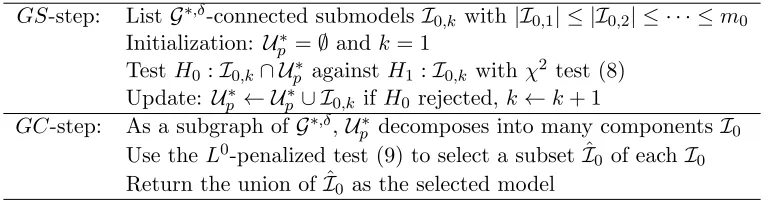
GS-step: ListG∗,δ-connected submodels I
0,k with|I0,1| ≤ |I0,2| ≤ · · · ≤m0 Initialization: Up∗ =∅and k= 1
TestH0 :I0,k∩ Up∗ against H1 :I0,k withχ2 test (8)
Update: Up∗ ← Up∗∪ I0,k ifH0 rejected, k←k+ 1
GC-step: As a subgraph ofG∗,δ,U∗
p decomposes into many components I0 Use theL0-penalized test (9) to select a subset ˆI0 of eachI0 Return the union of ˆI0 as the selected model
Table 1: Graphlet Screening Algorithm.
over all |I0| ×1 vectors ξ, each nonzero coordinate of which ≥ vgs in magnitude. The resultant estimator is the final estimate of GS, and we use ˆβgs= ˆβgs(Y;δ,Q, ugs, vgs, X, p, n) to denote it. See Section 1.5 for notations used in this paragraph.
Sometimes for linear models with random designs, the Gram matrixGis very noisy, and GS is more effective if we use it iteratively for a few times (≤5). This can be implemented in a similar way as that in Ji and Jin (2011, Section 3). Here, the main purpose of iteration is to denoise G, not for variable selection. See Ji and Jin (2011, Section 3) and Section 4 for more discussion.
2.2 Computational Complexity
If we exclude the overhead of obtainingG∗,δ, then the computation cost of GS contains two
parts, that of the GS-step and that of the GC-step. In each part, the computation cost hinges on the sparsity of G∗,δ. In Section 2.3, we show that with a properly chosen δ, for
a wide class of design matrices, G∗,δ is K-sparse for some K =K
p ≤Clogα(p) asp → ∞,
whereα >0 is a constant. As a result (Frieze and Molloy, 1999),
|A(m0)| ≤pm0(eKp)m0 ≤Cm0plogm0α(p). (10) We now discuss two parts separately.
In the GS-step, the computation cost comes from that of listing all elements in A(m0), and that of screening all connected-subgraphs inA(m0). Fix 1≤k≤m0. By (10) and the fact that every sizek(k >1) connected subgraph at least contains one sizek−1 connected subgraph, greedy algorithm can be used to list all sub-graphs with sizekwith computational complexity≤Cp(Kpk)k≤Cplogkα(p), and screening all connected subgraphs of sizekhas
computational complexity≤Cnplogkα(p). Therefore, the computational complexity of the GS-step≤Cnp(log(p))(m0+1)α.
The computation cost of theGC-step contains the part of breakingU∗
p into disconnected
components, and that of cleaning each component by minimizing (9). As a well-known appli-cation of the breadth-first search (Hopcroft and Tarjan, 1973), the first part≤ |Up∗|(Kp+ 1).
For the second part, by the SAS property of theGS-step (i.e., Lemma 16), for a broad class of design matrices, with the tuning parameters chosen properly, there is a fixed integer
total computational cost of the GC-step is no greater than C(2`0logα(p))|U∗
p|n, which is
moderate.
The computational complexity of GS is only moderately larger than that of Univari-ate Screening or UPS (Ji and Jin, 2011). UPS uses univariUnivari-ate thresholding for screen-ing which has a computational complexity of O(np), and GS implements multivariate screening for all connected subgraphs in A(m0), which has a computational complexity ≤Cnp(log(p))(m0+1)α. The latter is only larger by a multi-log(p) term.
2.3 Asymptotic Rare and Weak Model and Random Design Model
To analyze GS, we consider the regression model Y = Xβ +σz as in (1), and use an Asymptotic Rare and Weak (ARW) model for β and a random design model forX.
We introduce the ARW first. Fix parameters ∈ (0,1), τ > 0, and a ≥ 1. Let
b= (b1, . . . , bp)0 be thep×1 random vector where bi
iid
∼ Bernoulli(). (11)
We model the signal vector β in Model (1) by
β=b◦µ, (12)
where “◦” denotes the Hadamard product (see Section 1.5) andµ∈Θ∗
p(τ, a), with
Θ∗p(τ, a) ={µ∈Θp(τ),kµk∞≤aτ}, Θp(τ) ={µ∈Rp : |µi| ≥τ,1≤i≤p}. (13)
In this model,calibrates the sparsity level and τ calibrates the minimum signal strength. We are primarily interested in the case where is small andτ is smaller than the required signal strength for the exact recovery of the support of β, so the signals are both rare and weak. The constraint ofkµk∞≤aτpis mainly for technical reasons (only needed for Lemma
16); see Section 2.6 for more discussions.
We let p be the driving asymptotic parameter, and tie (, τ) to p through some fixed parameters. In detail, fixing 0< ϑ <1, we model
=p=p−ϑ. (14)
For any fixed ϑ, the signals become increasingly sparser as p→ ∞. Also, as ϑranges, the sparsity level ranges from very dense to very sparse, and covers all interesting cases.
It turns out that the most interesting range for τ is τ = τp = O(
p
log(p)). In fact, when τp σ
p
log(p), the signals are simply too rare and weak so that successful variable selection is impossible. On the other hand, exact support recovery requires τ &σ√2 logp
for orthogonal designs and possibly even larger τ for correlated designs. In light of this, we fixr >0 and calibrate τ by
τ =τp=σ
p
2rlog(p). (15)
For any positive definite matrix A, let λ(A) be the smallest eigenvalue, and let
λ∗k(Ω) = min{λ(A) :Ais a k×kprinciple submatrix of Ω}. (16)
Form0 as in the GS-step, let g=g(m0, ϑ, r) be the smallest integer such that
g≥max{m0,(ϑ+r)2/(2ϑr)}. (17) Fixing a constant c0>0, introduce
Mp(c0, g) ={Ω :p×p correlation matrix,λ∗g(Ω)≥c0}. (18) RecallXi is thei-th row ofX; see (2). In the random design model, we fix an Ω∈ M(c0, g) (Ω is unknown to us), and assume
Xi iid
∼N(0,1
nΩ), 1≤i≤n. (19)
In the literature, this is called the Gaussian design, which can be found in Compressive Sensing (Bajwa et al., 2007), Computer Security (Dinur and Nissim, 2003), and other ap-plication areas.
At the same time, fixing κ∈(0,1), we model the sample sizen by
n=np =pκ. (20)
Asp→ ∞,np becomes increasingly large but is still much smaller thanp. We assume
κ >(1−ϑ), (21)
so thatnp pp. Notepp is approximately the total number of signals. Condition (21) is
almost necessary for successful variable selection (Donoho, 2006a,b).
Definition 4 We call model (11)-(15) for β the Asymptotic Rare Weak model ARW(ϑ, r, a, µ), and call model (19)-(21) for X the Random Design modelRD(ϑ, κ,Ω).
2.4 Minimax Hamming Distance
In many works on variables selection, one assesses the optimality by the ‘oracle property’, where the probability of non-exact recoveryP(sgn( ˆβ)6= sgn(β)) is the loss function. When signals are rare and weak,P(sgn( ˆβ)6= sgn(β))≈1 and ‘exact recovery’ is usually impossible. A more appropriate loss function is the Hamming distance between sgn( ˆβ) and sgn(β).
For any fixed β and any variable selection procedure ˆβ, we measure the performance by the Hamming distance:
hp( ˆβ, β
X) =E hXp
j=1 1
sgn( ˆβj)6= sgn(βj) X i
.
In the Asymptotic Rare Weak model,β =b◦µ, and (p, τp) depend onpthrough (ϑ, r), so
the overall Hamming distance for ˆβ is
Hp( ˆβ;p, np, µ,Ω) =EpEΩ
hp( ˆβ, β
X)
≡EpEΩ
hp( ˆβ, b◦µ
X)
where Ep is the expectation with respect to the law of b, and EΩ is the expectation with respect to the law ofX; see (11) and (19). Finally, the minimax Hamming distance is
Hamm∗p(ϑ, κ, r, a,Ω) = inf ˆ
β
sup
µ∈Θ∗
p(τp,a)
Hp( ˆβ;p, np, µ,Ω) .
The Hamming distance is no smaller than the sum of the expected number of signal com-ponents that are misclassified as noise and the expected number of noise comcom-ponents that are misclassified as signal.
2.5 Lower Bound for the Minimax Hamming Distance, and GOLF
We first construct lower bounds for “local risk” at differentj, 1≤j≤p, and then aggregate them to construct a lower bound for the global risk. One challenge we face is the least favorable configurations for differentjoverlap with each other. We resolve this by exploiting the sparsity of a new graph to be introduced: Graph of Least Favorable (GOLF).
To recap, the model we consider is Model (1), where
β is modeled by ARW(ϑ, r, a, µ), and X is modeled by RD(ϑ, κ,Ω).
Fix 1≤j ≤p. The “local risk” at an index j is the risk of estimating the set of variables {βk : d(k, j) ≤ g}, where g is defined in (17) and d(j, k) denotes the geodesic distance
betweenj andk in the graphG∗,δ. The goal is to construct two subsetsV
0 andV1 and two realizations ofβ,β(0) and β(1) such that j∈V0∪V1 and
Ifk /∈V0∪V1,βk(0) =βk(1); otherwise,β(ki)6= 0 if and only if k∈Vi,i= 0,1,
where in the special case of V0 = V1, we require sgn(β(0)) 6= sgn(β(1)). In the literature, it is known that how well we can estimate {βk :d(k, j) ≤g} depends on how well we can
separate two hypotheses (where β(0) and β(1) are assumed as known):
H0(j):Y =Xβ(0)+σz vs. H1(j):Y =Xβ(1)+σz, z∼N(0, In). (22)
The least favorable configuration for the local risk at indexjis the quadruple (V0, V1, β(0), β(1)) for which two hypotheses are the most difficult to separate.
For anyV ⊂ {1,2, . . . , p}, letIV be the indicator vector ofV such that for any 1≤k≤p,
thek-th coordinate of IV is 1 ifk∈V and is 0 otherwise. Define
BV ={IV ◦µ: µ∈Θ∗p(τp, a)},
where we recall “◦” denotes the Hadamard product (see Section 1.5). Denote for short
θ(i) =IV0∪V1◦β
(i), and so β(1)−β(0) =θ(1)−θ(0) and θ(i)∈B
Vi,i= 0,1. Introduce
α(θ(0), θ(1)) =α(θ(0), θ(1);V0, V1,Ω, a) =τp−2(θ(0)−θ(1))
0
Ω(θ(0)−θ(1)).
For the testing problem in (22), the optimal test is to reject H0(j) if and only if (θ(1)−
θ(0))0X0(Y −Xβ(0))≥tστ
p
p
(θ(0)−θ(1))0Ω(θ(0)−θ(1)), since the support of θ(0)−θ(1) is contained in a small-size set
V0∪V1. Therefore the sum of Type I and Type II error of any test associated with (22) is no smaller than (up to some negligible differences)
|V0|
p Φ(¯ t) +
|V1|
p Φ t−(τp/σ)[α(θ(0), θ(1))]1/2
, (23)
where ¯Φ = 1−Φ is the survival function of N(0,1).
For a lower bound for the “local risk” at j, we first optimize the quantity in (23) over all θ(0) ∈ BV0 and θ
(1) ∈ B
V1, and then optimize over all (V0, V1) subject to j ∈ V0 ∪V1.
To this end, define α∗(V0, V1) = α∗(V0, V1;a,Ω), η(V0, V1) = η(V0, V1;ϑ, r, a,Ω), and ρ∗j = ρ∗j(ϑ, r, a,Ω) by
α∗(V0, V1) = min
α(θ(0), θ(1);V0, V1,Ω, a) : θ(i)∈BVi, i= 0,1,sgn(θ
(0))6= sgn(θ(1))}, (24)
η(V0, V1) = max{|V0|,|V1|}ϑ+ 1 4
" p
α∗(V
0, V1)r−
(|V1| − |V0|) ϑ p
α∗(V 0, V1)r
!
+
#2
,
and
ρ∗j(ϑ, r, a,Ω) = min {(V0,V1):j∈V1∪V0}
η(V0, V1).
The following shorthand notation is frequently used in this paper, which stands for a generic multi-log(p) term that may vary from one occurrence to another.
Definition 5 Lp >0 denotes a multi-log(p) term such that when p → ∞, for any δ > 0, Lppδ→ ∞ and Lpp−δ →0.
By (23) and Mills’ ratio (Wasserman and Roeder, 2009), a lower bound for the “local risk” atj is
sup {(V0,V1):j∈V0∪V1}
inf
t
|V0|
p Φ(¯ t) +
|V1|
p Φ t−(τp/σ)[α∗(V0, V1)]1/2
= sup
{(V0,V1):j∈V0∪V1}
Lpexp −η(V0, V1)·log(p) =Lpexp(−ρ∗j(ϑ, r, a,Ω) log(p)).
We now aggregate such lower bounds for “local risk” for a global lower bound. Since the “least favorable” configurations of (V0, V1) for different j may overlap with each other, we need to consider a graph as follows. Revisit the optimization problem in (24) and let
(V0∗j, V1∗j) = argmin{(V0,V1):j∈V1∪V0}η(V0, V1;ϑ, r, a,Ω). (25)
When there is a tie, pick the pair that appears first lexicographically. Therefore, for any 1 ≤ j ≤ p, V0∗j ∪V1∗j is uniquely defined. In Lemma 22 of the appendix, we show that |V0∗j ∪V1∗j| ≤(ϑ+r)2/(2ϑr) for all 1≤j≤p.
We now define a new graph, Graph of Least Favorable (GOLF), G = (V, E), where
Theorem 6 Fix (ϑ, κ) ∈ (0,1)2, r > 0, and a ≥ 1 such that κ > (1 −ϑ), and let Mp(c0, g) be as in (18). Consider Model (1) where β is modeled by ARW(ϑ, r, a, µ) and
X is modeled by RD(ϑ, κ,Ω) and Ω ∈ Mp(c0, g) for sufficiently large p. Then as p → ∞, Hamm∗p(ϑ, κ, r, a,Ω)≥Lp
dp(G)
−1Pp
j=1p
−ρ∗j(ϑ,r,a,Ω).
A similar claim holds for deterministic design models; the proof is similar so we omit it.
Corollary 7 For deterministic design models, the parallel lower bound holds for the mini-max Hamming distance withΩ replaced byG in the calculation ofρ∗j(ϑ, r, a,Ω)and dp(G).
Remark. The lower bounds contain a factor of
dp(G)
−1
. In many cases including that considered in our main theorem (Theorem 8), this factor is a multi-log(p) term so it does not have a major effect. In some other cases, the factor
dp(G)
−1
could be much smaller, say, when the GOSD has one or a few hubs, the degrees of which grow algebraically fast as p grows. In these cases, the associated GOLF may (or may not) have large-degree hubs. As a result, the lower bounds we derive could be very conservative, and can be substantially improved if we treat the hubs, neighboring nodes of the hubs, and other nodes separately. For the sake of space, we leave such discussion to future work.
Remark. A similar lower bound holds if the conditionµ∈Θ∗
p(τp, a) of ARW is replaced
byµ∈Θp(τp). In (24), suppose we replace Θp∗(τp, a) by Θp(τp), and the minimum is achieved
at (θ(0), θ(1)) = (θ∗(0)(V0, V1; Ω), θ(1)∗ (V0, V1; Ω)). Let g=g(m0, ϑ, r) be as in (17) and define
a∗g(Ω) = max {(V0,V1):|V0∪V1|≤g}
{kθ(0)∗ (V0, V1; Ω)k∞,kθ∗(1)(V0, V1; Ω)k∞}.
By elementary calculus, it is seen that for Ω∈ Mp(c0, g), there is a a constantC=C(c0, g) such thata∗g(Ω)≤C. If additionally we assume
a > a∗g(Ω), (26)
thenα∗(V0, V1) =α∗(V0, V1; Ω, a),η(V0, V1; Ω, a, ϑ, r), andρ∗j(ϑ, r, a,Ω) do not depend ona.
Especially, we can derive an alternative formula forρ∗j(ϑ, r, a,Ω); see Lemma 18 for details. When (26) holds, Θ∗p(τp, a) is broad enough in the sense that the least favorable
config-urations (V0, V1, β(0), β(1)) for all j satisfy kβ(i)k∞ ≤ aτp, i = 0,1. Consequently, neither
the minimax rate nor GS needs to adapt toa. In Section 2.6, we assume (26) holds; (26) is a mild condition for it only involves small-size sub-matrices of Ω.
2.6 Upper Bound and Optimality of Graphlet Screening
Fix constantsγ ∈(0,1) andA >0. LetMp(c0, g) be as in (18). In this section, we further restrict Ω to the following set:
M∗p(γ, c0, g, A) =
n
Ω∈ Mp(c0, g) :
p
X
j=1
|Ω(i, j)|γ≤A, 1≤i≤p
o
.
Note that any Ω ∈ M∗
In GS, when we regularize GOSD as in (4), we set the threshold δ by
δ =δp = 1/log(p). (27)
Such a choice for threshold is mainly for convenience, and can be replaced by any term that tends to 0 logarithmically fast asp→ ∞.
For any subsets D and F of{1,2, . . . , p}, defineω(D, F; Ω) =ω(D, F;ϑ, r, a,Ω, p) by
ω(D, F; Ω) = min
ξ∈R|D|,mini∈D|ξi|≥1
n
ξ0 ΩD,D−ΩD,F(ΩF,F)−1ΩF,D
ξo, (28)
Writeω =ω( ˆD,Fˆ; Ω) for short. We choose the tuning parameters in theGS-step in a way such that
t( ˆD,Fˆ) = 2σ2q( ˆD,Fˆ) logp, (29) whereq =q( ˆD,Fˆ)>0 satisfies
√
q0≤ √
q ≤√ωr−
q
(ϑ+ωr)2
4ωr −
|Dˆ|+1
2 ϑ, |Dˆ|is odd & ωr/ϑ >|Dˆ|+ (|Dˆ|
2−1)1/2, √
q0≤ √
q ≤√ωr−
q
1 4ωr−
1
2|Dˆ|ϑ, |Dˆ|is even & ωr/ϑ≥2|Dˆ|,
q is a constant such that q≥q0, otherwise.
(30) We set the GC-step tuning parameters by
ugs =σp2ϑlogp, vgs=τp=σ
p
2rlogp. (31)
The main theorem of this paper is the following theorem.
Theorem 8 Fix m0 ≥1, (ϑ, γ, κ)∈(0,1)3, r >0, c0 >0, g >0, a >1, A >0 such that
κ >1−ϑand (17) is satisfied. Consider Model (1) where β is modeled by ARW(ϑ, r, a, µ),
X is modeled byRD(ϑ, κ,Ω), and whereΩ∈ M∗p(γ, c0, g, A) and a > a∗g(Ω)for sufficiently
large p. Let βˆgs = ˆβgs(Y;δ,Q, ugs, vgs, X, p, n) be the Graphlet Screening procedure defined as in Section 2.1, where the tuning parameters (δ,Q, ugs, vgs) are set as in (27)-(31). Then
as p→ ∞, supµ∈Θ∗
p(τp,a)Hp( ˆβ gs;
p, np, µ,Ω)≤Lp
h
p1−(m0+1)ϑ+Pp
j=1p
−ρ∗j(ϑ,r,a,Ω)
i
+o(1).
Note thatρ∗j =ρ∗j(ϑ, r, a,Ω) does not depend ona. Also, note that in the most interesting range, Pp
j=1p
−ρ∗j 1. So if we choose m
0 properly large, e.g., (m0 + 1)ϑ > 1, then supµ∈Θ∗
p(τp,a)Hp( ˆβ gs;
p, np, µ,Ω) ≤ LpPpj=1p−ρ ∗
j(ϑ,r,a,Ω). Together with Theorem 6, this says that GS achieves the optimal rate of convergence, adaptively to all Ω inM∗
p(γ, c0, g, A) and β ∈Θ∗p(τp, a). We call this property optimal adaptivity. Note that since the diagonals
of Ω are scaled to 1 approximately,κ≡log(np)/log(p) does not have a major influence over
the convergence rate, as long as (21) holds.
Remark. Theorem 8 addresses the case where (26) holds so a > a∗g(Ω). We now briefly discuss the case wherea < a∗g(Ω). In this case, the set Θ∗p(τp, a) becomes sufficiently
narrow and a starts to have some influence over the optimal rate of convergence, at least for some choices of (ϑ, r). To reflect the role of a, we modify GS as follows: (a) in the
GS-step, replacing the χ2-screening by the likelihood based screening procedure; that is, when we screen I0= ˆD∪Fˆ, we accept nodes in ˆDonly when h( ˆF)> h(I0), where for any subset D ⊂ {1,2, . . . , p}, h(D) = min1
2kP
D(Y −X⊗,Dξ)k2 +ϑσ2log(p)|D| , where the minimum is computed over all|D|×1 vectorsξwhose nonzero elements all have magnitudes in [τp, aτp]. From a practical point of view, this modified procedure depends more on the
underlying parameters and is harder to implement than is GS. However, this is the price we need to pay whena is small. Since we are primarily interested in the case of relatively largera wherea > a∗g(Ω) holds, we skip further discussion along this line.
2.7 Phase Diagram and Examples Where ρ∗j(ϑ, r, a,Ω) Have Simple Forms
In general, the exponentsρ∗j(ϑ, r, a,Ω) may depend on Ω in a complicated way. Still, from time to time, one may want to find a simple expression forρ∗j(ϑ, r, a,Ω). It turns out that in a wide class of situations, simple forms for ρ∗j(ϑ, r, a,Ω) are possible. The surprise is that, in many examples, ρ∗j(ϑ, r, a,Ω) depends more on the trade-off between the parameters ϑ
and r (calibrating the signal sparsity and signal strength, respectively), rather than on the large coordinates of Ω.
We begin with the following theorem, which is proved in Ji and Jin (2011, Theorem 1.1).
Theorem 9 Fix (ϑ, κ)∈(0,1),r >0, anda >1such thatκ >(1−ϑ). Consider Model (1) where β is modeled byARW(ϑ, r, a, µ) and X is modeled byRD(ϑ, κ,Ω). Then as p→ ∞,
Hamm∗p(ϑ, κ, r, a,Ω)
p1−ϑ &
1, 0< r < ϑ,
Lpp−(r−ϑ)
2/(4r)
, r > ϑ.
Note thatp1−ϑis approximately the number of signals. Therefore, whenr < ϑ, the number of selection errors can not get substantially smaller than the number of signals. This is the most difficult case where no variable selection method can be successful.
In this section, we focus on the case r > ϑ, so that successful variable selection is possible. In this case, Theorem 9 says that a universal lower bound for the Hamming distance is Lpp1−(ϑ+r)
2/(4r)
. An interesting question is, to what extend, this lower bound is tight.
Recall thatλ∗k(Ω) denotes the minimum of smallest eigenvalues across allk×kprinciple submatrices of Ω, as defined in (16). The following corollaries are proved in Section 6.
Corollary 10 Suppose the conditions of Theorem 8 hold, and that additionally,1< r/ϑ <
3 + 2√2 ≈ 5.828, and |Ω(i, j)| ≤ 4√2−5 ≈ 0.6569 for all 1 ≤ i, j ≤ p, i 6= j. Then as
p→ ∞, Hamm∗p(ϑ, κ, r, a,Ω) =Lpp1−(ϑ+r)
2/(4r)
.
Corollary 11 Suppose the conditions of Theorem 8 hold. Also, suppose that 1 < r/ϑ <
5 + 2√6 ≈ 9.898, and that λ∗3(Ω) ≥ 2(5−2√6) ≈ 0.2021, λ∗4(Ω) ≥ 5−2√6 ≈ 0.1011, and |Ω(i, j)| ≤ 8√6− 19 ≈ 0.5959 for all 1 ≤ i, j ≤ p, i 6= j. Then as p → ∞, Hamm∗p(ϑ, κ, r, a,Ω) =Lpp1−(ϑ+r)
2/(4r)
.
0 0.5 1 0
1 2 3 4
ϑ
r
Exact Recovery
Almost Full Recovery
No Recovery
0 0.5 1
0 1 2 3 4
ϑ
r
Exact Recovery
Almost Full Recovery
No Recovery
0 0.5 1
0 1 2 3 4
ϑ
r
Exact Recovery
Almost Full Recovery
No Recovery
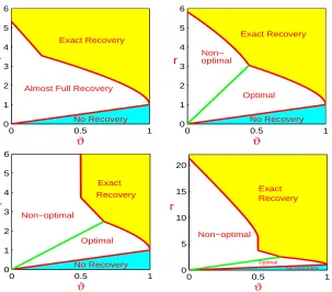
Figure 1: Phase diagram for Ω = Ip (left), for Ω satisfying conditions of Corollary 10
(middle), and for Ω satisfying conditions of Corollary 11 (right). Red line: r =ϑ. Solid red curve: r =ρ(ϑ,Ω). In each of the last two panels, the blue line intersects with the red curve at (ϑ, r) = (1/2,[3 + 2√2]/2) (middle) and (ϑ, r) = (1/3,[5 + 2√6]/3) (right), which splits the red solid curve into two parts; the part to the left is illustrative for it depends on Ω in a complicated way; the part to the right, together with the dashed red curve, representr= (1+√1−ϑ)2(in the left panel, this is illustrated by the red curve).
Note also that by Theorem 8, under the condition of either Corollaries 10 or Corollary 11, GS achieves the optimal rate in that
sup
µ∈Θ∗
p(τp,a)
Hp( ˆβgs;p, np, µ,Ω)≤Lpp1−(ϑ+r)
2/(4r)
. (32)
Together, Theorem 9, Corollaries 10-11, and (32) have an interesting implication on the so-calledphase diagram. Call the two-dimensionalparameter space{(ϑ, r) : 0< ϑ <1, r >0} the phase space. There are two curves r = ϑ and r = ρ(ϑ,Ω) (the latter can be thought of as the solution of Pp
j=1p
−ρ∗j(ϑ,r,a,Ω) = 1; recall that ρ∗
j(ϑ, r, a,Ω) does not depend ona)
that partition the whole phase space into three different regions:
• Region of No Recovery. {(ϑ, r) : 0 < r < ϑ,0 < ϑ <1}. In this region, as p → ∞, for any Ω and any procedures, the minimax Hamming error equals approximately to the total expected number of signals. This is the most difficult region, in which no procedure can be successful in the minimax sense.
• Region of Almost Full Recovery. {(ϑ, r) :ϑ < r < ρ(ϑ,Ω)}. In this region, asp→ ∞, the minimax Hamming distance satisfies 1 Hamm∗p(ϑ, κ, r, a,Ω) p1−ϑ, and it is possible to recover most of the signals, but it is impossible to recover all of them.
In general, the functionρ(ϑ,Ω) depends on Ω in a complicated way. However, by Theorem 9 and Corollaries 10-11, we have the following conclusions. First, for all Ω and a > 1,
ρ(ϑ,Ω) ≥ (1 +√1−ϑ)2 for all 0 < ϑ < 1. Second, in the simplest case where Ω = I
p,
Hamm∗p(ϑ, κ, r, a,Ω) = Lpp1−(ϑ+r)
2/(4r)
, and ρ(ϑ,Ω) = (1 +√1−ϑ)2 for all 0 < ϑ < 1. Third, under the conditions of Corollary 10, ρ(ϑ,Ω) = (1 +√1−ϑ)2 if 1/2< ϑ <1. Last, under the conditions of Corollary 11, ρ(ϑ,Ω) = (1 +√1−ϑ)2 if 1/3 < ϑ < 1. The phase diagram for the last three cases are illustrated in Figure 1. The blue lines arer/ϑ= 3+2√2 (middle) andr/ϑ= 5 + 2√6 (right).
Corollaries 10-11 can be extended to more general situations, where r/ϑmay get arbi-trary large, but consequently, we need stronger conditions on Ω. Towards this end, we note that for any (ϑ, r) such that r > ϑ, we can find a unique integer N = N(ϑ, r) such that 2N −1≤(ϑ/r+r/ϑ)/2<2N+ 1. Suppose that for any 2≤k≤2N −1,
λ∗k(Ω)≥ max
{(k+1)/2≤j≤min{k,N}}
n(r/ϑ+ϑ/r)/2−2j+ 2 +p[(r/ϑ+ϑ/r)/2−2j+ 2]2−1
(2k−2j+ 1)(r/ϑ)
o
,
(33) and that for any 2≤k≤2N,
λ∗k(Ω)≥ max {k/2≤j≤min{k−1,N}}
n(r/ϑ+ϑ/r)/2 + 1−2j
(k−j)(r/ϑ)
o
. (34)
Then we have the following corollary.
Corollary 12 Suppose the conditions in Theorem 8 and that in (33)-(34) hold. Then as
p→ ∞, Hamm∗p(ϑ, κ, r, a,Ω) =Lpp1−(ϑ+r)
2/(4r)
.
The right hand sides of (33)-(34) decrease with (r/ϑ). For a constants0 >1, (33)-(34) hold for all 1< r/ϑ≤s0 as long as they hold for r/ϑ=s0. Hence Corollary 12 implies a similar partition of the phase diagram as do Corollaries 10-11.
Remark. Phase diagram can be viewed as a new criterion for assessing the optimality, which is especially appropriate for rare and weak signals. The phase diagram is a partition of the phase space {(ϑ, r) : 0< ϑ <1, r >0}into different regions where statistical inferences are distinctly different. In general, a phase diagram has the following four regions:
• An “exact recovery” region corresponding to the “rare and strong” regime in which high probability of completely correct variable selection is feasible.
• An “almost full recovery” region as a part of the “rare and weak” regime in which completely correct variable selection is not achievable with high probability but vari-able selection is still feasible in the sense that with high probability, the number of incorrectly selected variables is a small fraction of the total number of signals.
• A “detectable” region in which variable selection is infeasible but the detection of the existence of a signal (somewhere) is feasible (e.g., by the Higher Criticism method).
In the sparse signal detection (Donoho and Jin, 2004) and classification (Jin, 2009) problems, the main interest is to find the detectable region, so that the exact recovery and almost full recovery regions were lumped into a single “estimable” region (e.g., Donoho and Jin, 2004, Figure 1). For variable selection, the main interest is to find the boundaries of the almost full discovery region so that the detectable and non-detectable regions are lumped into a single “no recovery” region as in Ji and Jin (2011) and Figure 1 of this paper.
Variable selection in the “almost full recovery” region is a new and challenging problem. It was studied in Ji and Jin (2011) when the effect of signal cancellation is negligible, but the hardest part of the problem was unsolved in Ji and Jin (2011). This paper (the second in this area) deals with the important issue of signal cancellation, in hopes of gaining a much deeper insight on variable selection in much broader context.
2.8 Non-optimality of Subset Selection and the Lasso
Subset selection (also called theL0-penalization method) is a well-known method for vari-able selection, which selects varivari-ables by minimizing the following functional:
1
2kY −Xβk 2+ 1
2(λss) 2kβk
0, (35)
wherekβkq denotes theLq-norm,q ≥0, andλss>0 is a tuning parameter. The AIC, BIC,
and RIC are methods of this type (Akaike, 1974; Schwarz, 1978; Foster and George , 1994). Subset selection is believed to have good “theoretic property”, but the main drawback of this method is that it is computationally NP hard. To overcome the computational challenge, many relaxation methods are proposed, including but are not limited to the lasso (Chen et al., 1998; Tibshirani, 1996), SCAD (Fan and Li, 2001), MC+ (Zhang, 2010), and Dantzig selector (Candes and Tao, 2007). Take the lasso for example. The method selects variables by minimizing
1
2kY −Xβk 2+λ
lassokβk1, (36)
where the L0-penalization is replaced by the L1-penalization, so the functional is convex and the optimization problem is solvable in polynomial time under proper conditions.
Somewhat surprisingly, subset selection is generally rate non-optimal in terms of selec-tion errors. This sub-optimality of subset selecselec-tion is due to its lack of flexibility in adapting to the “local” graphic structure of the design variables. Similarly, other global relaxation methods are sub-optimal as well, as the subset selection is the “idol” these methods try to mimic. To save space, we only discuss subset selection and the lasso, but a similar conclusion can be drawn for SCAD, MC+, and Dantzig selector.
For mathematical simplicity, we illustrate the point with an idealized regression model where the Gram matrixG=X0X is diagonal block-wise and has 2×2 blocks
At the same time, we continue to model β with the Asymptotic Rare and Weak model ARW(ϑ, r, a, µ), but where we relax the assumption ofµ∈Θ∗p(τp, a) to that of µ∈Θp(τp)
so that the strength of each signal ≥ τp (but there is no upper bound on the strength).
Consider a variable selection procedure ˆβ?, where?=gs, ss, lasso, representing GS, subset selection, and the lasso and the tuning parameters for each method are ideally set. Note that for the worst-case risk considered below, the ideal tuning parameters depend on (ϑ, r, p, h0) but do not depend on µ. Since the index groups {2j −1,2j} are exchangeable in (37) and the ARW models, the Hamming error of β? in its worst case scenario has the form of sup{µ∈Θp(τp)}Hp( ˆβ
?;
p, µ, G) =Lpp1−ρ?(ϑ,r,h0).
We now study ρ?(ϑ, r, h0). Towards this end, we first introduce ρ(3)lasso(ϑ, r, h0) =
(2|h0|)−1[(1−h20) √
r −p
(1−h20)(1− |h0|)2r−4|h0|(1− |h0|)ϑ] 2
and ρ(4)lasso(ϑ, r, h0) =
ϑ+(1−|h0|)3(1+|h0|)
16h2 0
(1 +|h0|) √
r−p
(1− |h0|)2r−4|h0|ϑ/(1−h20)
2
. We then let
ρ(1)ss(ϑ, r, h0) =
2ϑ, r/ϑ≤2/(1−h20)
[2ϑ+ (1−h20)r]2/[4(1−h2
0)r], r/ϑ >2/(1−h20)
,
ρ(2)ss(ϑ, r, h0) =
2ϑ, r/ϑ≤2/(1− |h0|)
2[p2(1− |h0|)r−
p
(1− |h0|)r−ϑ]2, r/ϑ >2/(1− |h0|)
,
ρ(1)lasso(ϑ, r, h0) =
(
2ϑ, r/ϑ≤2/(1− |h0|)2
ρ(3)lasso(ϑ, r, h0), r/ϑ >2/(1− |h0|)2
,
and
ρ(2)lasso(ϑ, r, h0) =
(
2ϑ, r/ϑ≤(1 +|h0|)/(1− |h0|)3
ρ(4)lasso(ϑ, r, h0), r/ϑ >(1 +|h0|)/(1− |h0|)3
.
The following theorem is proved in Section 6.
Theorem 13 Fix ϑ ∈ (0,1) and r > 0 such that r > ϑ. Consider Model (1) where β
is modeled by ARW(ϑ, r, a, µ) and X satisfies (37). For GS, we set the tuning parameters (δ, m0) = (0,2), and set(Q, ugs, vgs) as in (29)-(31). For subset selection as in (35) and the lasso as in (36), we set their tuning parameters ideally given that (ϑ, r) are known. Then as p→ ∞,
ρgs(ϑ, r, h0) = min
(ϑ+r)2
4r , ϑ+
(1− |h0|)
2 r, 2ϑ+
{[(1−h20)r−ϑ]+}2 4(1−h2
0)r
, (38)
ρss(ϑ, r, h0) = min
(ϑ+r)2
4r , ϑ+
(1− |h0|) 2 r, ρ
(1)
ss(ϑ, r, h0), ρ(2)ss(ϑ, r, h0) , (39)
and
ρlasso(ϑ, r, h0) = min{
(ϑ+r)2 4r , ϑ+
(1− |h0|)r 2(1 +p
1−h2 0)
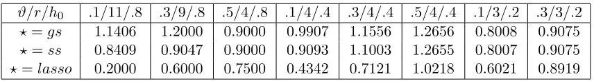
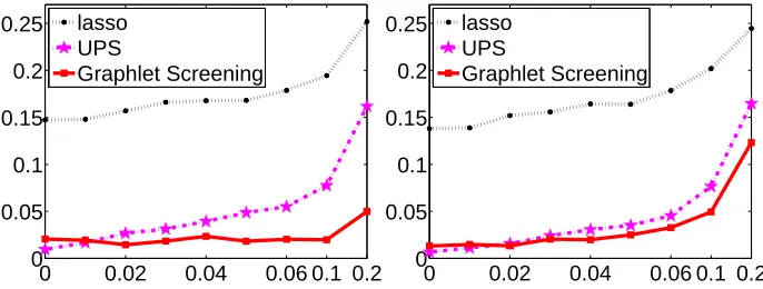
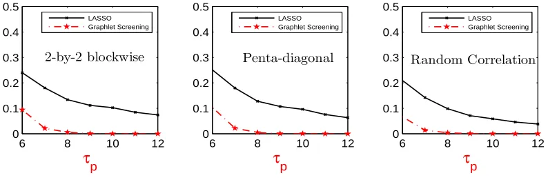
It can be shown that ρgs(ϑ, r, h0) ≥ ρss(ϑ, r, h0) ≥ ρlasso(ϑ, r, h0), where depending on the choices of (ϑ, r, h0), we may have equality or strict inequality (note that a larger exponent means a better error rate). This fits well with our expectation, where as far as the convergence rate is concerned, GS is optimal for all (ϑ, r, h0), so it outperforms the subset selection, which in turn outperforms the lasso. Table 2 summarizes the exponents for some representative (ϑ, r, h0). It is seen that differences between these exponents become increasingly prominent whenh0 increase and ϑdecrease.
ϑ/r/h0 .1/11/.8 .3/9/.8 .5/4/.8 .1/4/.4 .3/4/.4 .5/4/.4 .1/3/.2 .3/3/.2
?=gs 1.1406 1.2000 0.9000 0.9907 1.1556 1.2656 0.8008 0.9075
?=ss 0.8409 0.9047 0.9000 0.9093 1.1003 1.2655 0.8007 0.9075
?=lasso 0.2000 0.6000 0.7500 0.4342 0.7121 1.0218 0.6021 0.8919
Table 2: The exponentsρ?(ϑ, r, h0) in Theorem 13, where ?=gs, ss, lasso.
As in Section 2.7, each of these methods has a phase diagram plotted in Figure 2, where the phase space partitions into three regions: Region of Exact Recovery, Region of Almost Full Recovery, and Region of No Recovery. Interestingly, the separating boundary for the last two regions are the same for three methods, which is the line r = ϑ. The boundary that separates the first two regions, however, vary significantly for different methods. For any h0 ∈(−1,1) and ?=gs, ss, lasso, the equation for this boundary can be obtained by setting ρ?(ϑ, r, h0) = 1 (the calculations are elementary so we omit them). Note that the
lower the boundary is, the better the method is, and that the boundary corresponding to the lasso is discontinuous atϑ= 1/2. In the non-optimal region of either subset selection or the lasso, the Hamming errors of the procedure are much smaller thanpp, so the procedure
gives “almost full recovery”; however, the rate of Hamming errors is slower than that of the optimal procedure, so subset selection or the lasso is non-optimal in such regions.
Subset selection and the lasso are rate non-optimal for they are so-called one-step or non-adaptivemethods (Ji and Jin, 2011), which use only one tuning parameter, and which do not adapt to the local graphic structure. The non-optimality can be best illustrated with the diagonal block-wise model presented here, where each block is a 2×2 matrix. Correspondingly, we can partition the vectorβ into many size 2 blocks, each of which is of the following three types (i) those have no signal, (ii) those have exactly one signal, and (iii) those have two signals. Take the subset selection for example. To best separate (i) from (ii), we need to set the tuning parameter ideally. But such a tuning parameter may not be the “best” for separating (i) from (iii). This explains the non-optimality of subset selection.
Seemingly, more complicated penalization methods that use multiple tuning parameters may have better performance than the subset selection and the lasso. However, it remains open how to design such extensions to achieve the optimal rate for general cases. To save space, we leave the study along this line to the future.
2.9 Summary
0 0.5 1 0
1 2 3 4 5 6
ϑ
r
Exact Recovery
Almost Full Recovery
No Recovery
0 0.5 1
0 1 2 3 4 5 6
ϑ
r
Exact Recovery
Optimal Non−
optimal
No Recovery
0 0.5 1
0 1 2 3 4 5 6
ϑ
r
Exact Recovery
Optimal Non−optimal
No Recovery
0 0.5 1
0 5 10 15 20
ϑ
r
Exact Recovery
Optimal
Non−optimal
No Recovery
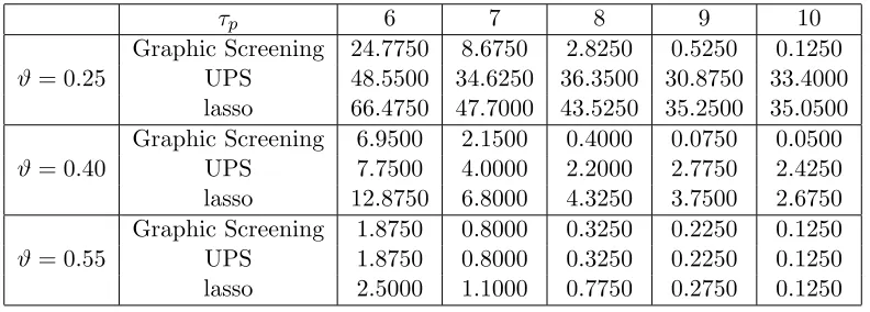
Figure 2: Phase diagrams for GS (top left), subset selection (top right), and the lasso (bottom; zoom-in on the left and zoom-out on the right), whereh0 = 0.5.
screening has a computation cost ofO(pm+np), GS only has a computation cost of Lpnp
(excluding the overhead of obtaining the GOSD), by utilizing graph sparsity. Note that when the design matrixGis approximately banded, say, all its large entries are confined to a diagonal band with bandwidth≤K, the overhead of GS can be reduced toO(npK). One such example is in Genome-Wide Association Study (GWAS), where G is the empirical Linkage Disequilibrium (LD) matrix, and K can be as small as a few tens. We remark that the lasso has a computational complexity of O(npk), where k, dominated by the number steps requiring re-evaluation of the correlation between design vectors and updated residuals, could be smaller than the Lp term for GS (Wang et al., 2013).
We use asymptotic minimaxity of the Hamming distance as the criterion for assessing optimality. Compared with existing literature on variable selection where we use theoracle propertyorprobability of exact support recoveryto assess optimality, our approach is math-ematically more demanding, yet scientifically more relevant in the rare/weak paradigm.