Conjugate Relation between Loss Functions and Uncertainty Sets in Classification Problems

Conjugate Relation between Loss Functions and Uncertainty Sets in

Classification Problems

Takafumi Kanamori [email protected]

Department of Computer Science and Mathematical Informatics Nagoya University

Nagoya 464-8603 Japan

Akiko Takeda [email protected]

Taiji Suzuki [email protected]

Department of Mathematical Informatics The University of Tokyo

Tokyo 113-8656, Japan

Editor:John Shawe-Taylor

Abstract

There are two main approaches to binary classification problems: the loss function approach and the uncertainty set approach. The loss function approach is widely used in real-world data analysis. Statistical decision theory has been used to elucidate its properties such as statistical consistency. Conditional probabilities can also be estimated by using the minimum solution of the loss function. In the uncertainty set approach, an uncertainty set is defined for each binary label from training samples. The best separating hyperplane between the two uncertainty sets is used as the decision function. Although the uncertainty set approach provides an intuitive understanding of learning algorithms, its statistical properties have not been sufficiently studied. In this paper, we show that the uncertainty set is deeply connected with the convex conjugate of a loss function. On the basis of the conjugate relation, we propose a way of revising the uncertainty set approach so that it will have good statistical properties such as statistical consistency. We also introduce statistical models corresponding to uncertainty sets in order to estimate conditional probabilities. Finally, we present numerical experiments, verifying that the learning with revised uncertainty sets improves the prediction accuracy.

Keywords: loss function, uncertainty set, convex conjugate, consistency

1. Introduction

(see Bartlett et al. 2006; Steinwart 2005, 2003; Schapire et al. 1998; Zhang 2004; Vapnik 1998 for details).

The loss function approach provides not only an estimator of the decision function, but also an estimator of the conditional probability of binary labels for a given input. The sign of the estimated decision function is used for the label prediction, and the magnitude of the decision function is connected to the conditional probability via the loss function. This connection has been studied by many researchers (Friedman et al., 1998; Bartlett and Tewari, 2007). For example, the logistic loss and exponential loss produce logistic models, whereas the hinge loss cannot be used to estimate the conditional probability except the probability 0.5 (Bartlett and Tewari, 2007).

Another approach to binary classification problems, the maximum-margin criterion, is taken in statistical learning. Under the maximum-margin criterion, the best separating hyperplane be-tween the two output labels is used as the decision function. Hard-margin SVM (Vapnik, 1998) defines a convex-hull of input vectors for each binary label, and takes into account the maximum-margin between the two convex-hulls. For the non-separable case,ν-SVM gives us a similar picture (Sch¨olkopf et al., 2000; Bennett and Bredensteiner, 2000). Ellipsoidal sets as well as polyhedral sets such as the convex-hull of finite input points can be used to solve classification problems (Lanckriet et al., 2003; Nath and Bhattacharyya, 2007). In this paper, the set used in the maximum-margin criterion is referred to as anuncertainty set. This term comes from the field of robust optimization in mathematical programming (Ben-Tal et al., 2009).

There have been studies on the statistical properties of learning with uncertainty sets. For ex-ample, Lanckriet et al. (2003) proposed minimax probability machine (MPM) using ellipsoidal uncertainty sets and studied its statistical properties in the worst-case setting. In statistical learning using uncertainty sets, the main concern is to develop optimization algorithms under the maximum margin criterion (Mavroforakis and Theodoridis, 2006). So far, however, the statistical properties of learning with uncertainty sets have not been studied as much as those of learning with loss functions. The main purpose of this paper is to study the relation between the loss function approach and uncertainty set approach, and to use the relation to transform learning with uncertainty sets into loss-based learning in order to clarify the statistical properties of learning algorithms. As men-tioned above, loss functions naturally involve statistical models of conditional probabilities. As a result, we can establish a correspondence between uncertainty sets and statistical models of condi-tional probabilities. Note that some of the existing learning methods using uncertainty sets do not necessarily have good statistical properties, such as the statistical consistency. We propose a way of revising uncertainty sets to establish statistical consistency.

Figure 1 shows how uncertainty sets, loss functions and statistical models are related. Starting from a learning algorithm with uncertainty sets, we obtain the corresponding loss function and statistical model via the convex conjugate. Usually, uncertainty sets are designed on the basis of an intuitive understandings of real-world data. By revising uncertainty sets, we can obtain the corresponding loss functions and statistical models. We also derive sufficient conditions under which the corresponding loss function produces a statistically consistent estimator. We think that our method of revising uncertainty sets can bridge the gap between intuitive statistical modeling and the nice statistical properties of learning algorithms.

☛

✡

✟

✠

Uncertainty sets

⇓

Uncertainty Set Revision: Sec. 4.2

⇑

Convex Conjugugate: Sec. 3.1

☛

✡

✟

✠

Loss Functions

☛

✡

✟

✠

Statistical Models

⇓

Loss Minimization: Sec. 3.2

Figure 1: Relations among uncertainty sets, loss functions and statistical models. In Section 3.1, we derive uncertainty sets from loss functions by using the convex conjugate of loss functions. In Section 3.2, we derive statistical models from loss functions. Section 4.2 shows how to revise uncertainty sets in order to obtain loss functions from them. By applying the relations in the diagram, we can transform learning with uncertainty sets into loss-based learning so that we can benefit from good statistical properties such as statistical consistency.

how to revising the uncertainty set so that it will have good statistical properties. Section 5 describes a based learning algorithm derived from uncertainty sets. Section 6 proves that the kernel-based algorithm has statistical consistency. The results of numerical experiments are described in Section 7. We conclude in section 8. The details of the proofs are shown in the Appendix.

Let us summarize the notations to be used throughout the paper. The indicator function is denoted as[[A]]; that is,[[A]]equals 1 ifAis true, and 0 otherwise. The column vectorxin Euclidean space is written in boldface. The transposition ofxis denoted asxT_{. The Euclidean norm of the} vectorxis expressed as_kx_k. For a setSin a linear space, the convex hull ofSis denoted as convS

or conv(S). The number of elements inSis denoted as_|S_|. The expectation of the random variable

Z w.r.t. the probability distributionPis described asE_{P[Z]. We will drop the subscript Pwhen it}

is clear from the context. The set of all measurable functions on the set

X

relative to the measure

Pis denoted byL0. The supremum norm of f ∈L0is denoted askfk∞. Elements in

X

are written in Roman alphabets such asx_∈

X

if

X

is not necessarily a subset of the Euclidean space. For the reproducing kernel Hilbert space

H

,_kf_kH is the norm of f _∈

H

defined from the inner product

h·,_·iH on

H

.

2. Preliminaries and Previous Studies

We define

X

as the input space and_{+1,₋1_}as the set of binary labels. Suppose that the training samples(x1,y1), . . . ,(xm,ym)∈

X

×{+1,−1}are drawn i.i.d. according to a probability distribution

Pon

X

× {+1,₋1_}. The goal is to estimate a decision function f :

X

→R_{such that the sign of}

decision function f is expected to be as small as possible.1 _{In this article, the composite function of}

the sign function and the decision function, sign(f(x)), is referred to as classifier.

2.1 Learning with Loss Functions

In binary classification problems, the prediction accuracy of the decision function f is measured by the 0-1 loss[[sign(f(x))₆=y]], which equals 1 when the sign of f(x) is different fromyand 0 otherwise.

The average prediction performance of the decision function f is evaluated by the expected 0-1 loss, that is,

E

(f) =E[ [[sign(f(x))₆=y]] ].

The Bayes risk

E

∗is defined as the minimum value of the expected 0-1 loss over all the measurable functions on

X

,

E

∗=inf_{

E

(f): f_∈L_0}. (1) The Bayes risk is the lowest achievable error rate given the probabilityP. Given a set of training samples,T =_{(x1,y1), . . . ,(xm,ym)}, the empirical 0-1 loss is expressed as

b

E

T(f) = 1

m

m

∑

i=1

[[sign(f(xi))6=yi]].

In what follows, the subscriptT in

E

bT(f)will be dropped if it is clear from the context.

In general, minimization of

E

bT(f)is a hard problem (Arora et al., 1997). The main difficulty comes from the non-convexity of the 0-1 loss[[sign(f(x))₆=y]]as a function of f. Hence, many learning algorithms use a surrogate loss in order to make the computation tractable. For example, SVM uses the hinge loss, max_{1₋y f(x),0_}, and Adaboost uses the exponential loss, exp_{−y f(x)_}. Both the hinge loss and the exponential loss are convex in f, and they provide an upper bound of the 0-1 loss. Thus, the minimizer under the surrogate loss is also expected to minimize the 0-1 loss. The quantitative relation between the 0-1 loss and the surrogate loss was studied by Bartlett et al. (2006) and Zhang (2004).

Regularization is used to avoid overfitting of the estimated decision function to the training sam-ples. The complexity of the estimated classifier is limited by adding a regularization term such as the squared norm of the decision function to an empirical surrogate loss. The balance between the regularization term and the surrogate loss is adjusted by using a regularization parameter (Evgeniou et al., 1999; Steinwart, 2005). Accordingly, regularization controls the deviation of the empirical loss from the expected loss. The optimization is computationally tractable when both the regular-ization term and the surrogate loss are convex.

Besides computational tractability, surrogate loss functions have another benefit. As discussed by Friedman et al. (1998) and Bartlett and Tewari (2007), surrogate loss functions provide statistical models for the conditional probability of a labelyfor a givenx, that is,P(y_|x). A brief introduction to this idea is given below.

Let us consider a minimization problem of the expected loss, minf∈L0E[ℓ(−y f(x))], where ℓ(₋y f(x))is a surrogate loss of a decision function f(x). The functionℓ:R_→R_{is assumed to be}

differentiable. In a similar way to Lemma 1 of Friedman et al. (1998), it is sufficient to minimize the loss function conditional onx:

E_{[ℓ(−y f(x))|x] =P(y= +1|x)ℓ(−f(x)) +P(y=−1|x)ℓ(f(x)).}

At the optimal solution, the derivative is equal to zero, that is,

∂

∂f(x)E[ℓ(−y f(x))|x] =−P(y= +1|x)ℓ

′_{(−f(x)) +P(y=−1|x)ℓ}′_(f(x)),

whereℓ′is the derivative ofℓ. Therefore, we have

P(y= +1_|x) = ℓ′(f(x)) ℓ′_{(f(x)) +ℓ}′_(−f(x))

for the optimal solution f. An estimator of the conditional probability can be obtained by substi-tuting an estimated decision function into the above expression. For example, the exponential loss exp_{−y f(x)_}yields the logistic model

P(y= +1_|x) = e f(x)

ef(x)_+e−f(x).

The relation between surrogate losses and statistical models was extensively studied by Bartlett and Tewari (2007).

2.2 Learning with Uncertainty Sets

Besides statistical learning using loss functions, there is another approach to binary classification problems, that is, statistical learning based on theuncertainty set. What follows is a brief introduc-tion to the basic idea of the uncertainty set. We assume that

X

is a subset of Euclidean space.

Uncertainty sets describe uncertainties or ambiguities present in robust optimization problems (Ben-Tal et al., 2009). The parameter in the optimization problem may not be precisely determined. For example, in portfolio optimization, the objective function may depend on a future stock price. Instead of precise information, we have an uncertainty set which probably includes the true pa-rameter of the optimization problem. Typically, the worst case is the setting in which the robust optimization problem with uncertainty sets is solved.

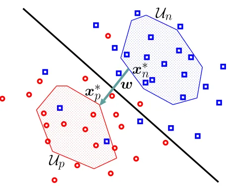
Statistical learning with uncertainty sets is an application of robust optimization to classification problems. An uncertainty set is prepared for each binary label. Each uncertainty set is assumed to include the mean vector of the distribution of input pointxconditioned on each label (Takeda et al., 2013). For example,

U

p and

U

n are confidence regions such that the conditional probabilities,

x

∗

n

x

∗

p

w

U

_p

U

_n

Figure 2: Decision boundary estimated by solving the minimum distance problem with the uncer-tainty sets

U

pand

U

n.

We use the uncertainty set to estimate the linear decision function f(x) =wT_{x+b. Here, let} us consider theminimum distance problem

min

xp,xnk

xp−xnk subject to xp∈

U

p,xn∈

U

n. (2)

Letx∗_p andx∗_n be optimal solutions of (2). Then, the normal vector of the decision function, w, can be estimated with c(x∗

p−x∗n), wherec is a positive real number. Figure 2 illustrates the es-timated decision boundary. When both

U

p and

U

n are compact subsets satisfying

U

p∩

U

n= /0, the estimated normal vector cannot be the null vector. The minimum distance problem appears in the hard margin SVM (Vapnik, 1998; Bennett and Bredensteiner, 2000),ν-SVM (Sch¨olkopf et al., 2000; Crisp and Burges, 2000) and the learning algorithms proposed by Nath and Bhattacharyya (2007) and Mavroforakis and Theodoridis (2006). Section 2.3 briefly describes the relation be-tweenν-SVM and the minimum distance problem. Another criterion is used to estimate the linear decision function in minimax probability machine (MPM) proposed by Lanckriet et al. (2003), but the ellipsoidal uncertainty set also plays an important role in MPM.

The minimum distance problem is equivalent to the maximum margin principle (Vapnik, 1998; Bennett and Bredensteiner, 2000). When the bias termbin the linear decision function is estimated such that the decision boundary bisects the line segment connectingx∗_p andx∗_n, the estimated de-cision boundary will have the maximum margin between the uncertainty sets,

U

pand

U

n. Takeda et al. (2013) studied the relation between the minimum distance problem and the maximum margin principle.

2.3 Loss Functions and Uncertainty Sets inν-SVM

Burges (2000) and Bennett and Bredensteiner (2000). We will extend this relation to more general learning algorithms in Section 3.

Suppose that the input space

X

is a subset of Euclidean space Rd_{, and we have the linear}

decision function, f(x) =wTx+b, where the normal vectorw_∈Rd _{and the bias termb∈}R_are

parameters to be estimated based on training samples. By applying the kernel trick (Berlinet and Thomas-Agnan, 2004; Sch¨olkopf and Smola, 2002), we can obtain rich statistical models for the decision function, while maintaining computational tractability.

The decision function used inν-SVM is estimated as the optimal solution of

min w,b,ρ

1 2kwk

2_−νρ+ 1 m

m

∑

i=1

max_{ρ₋yi(wTxi+b),0}, w∈Rd, b∈R,ρ∈R, (3)

whereν_∈(0,1)is a prespecified constant that acts as the regularization parameter. ν-SVM uses a variant of the hinge loss, max_{ρ₋yi(wTxi+b),0}, as a surrogate loss. As Sch¨olkopf et al. (2000) pointed out, the parameterνcontrols the margin errors and number of support vectors. Roughly speaking, the derivative of the objective function with respect toρyields

1

m

m

∑

i=1

[[yi(wTxi+b)<ρ]] =ν, (4)

where the subdifferential at ρ=yi(wTxi+b) has been ignored for simplicity. The left side of (4) is called the margin error. The quantity yi(wTxi+b) is referred to as the margin, and the equality above implies that an optimalρis theν-quantile of the empirical distribution of margins

yi(wTxi+b),i=1, . . . ,m. The empirical loss inν-SVM is minimized over training samples such thatyi(wTxi+b)<ρ, and training samples having a large margin, that is,yi(wTxi+b)≥ρ, do not contribute to the loss function max_{ρ₋yi(wTxi+b),0}. As a result, the sum of the second and third terms in ν-SVM (3) imply the mean of the negative margin ₋yi(wTxi+b) such that

yi(wTxi+b)<ρ, that is,

−νρ+1

m

m

∑

i=1

max_{ρ₋yi(wTxi+b),0}=ν· 1

mν_i:yi(wT

∑

_x i+b)<ρ

(₋yi(wTxi+b))

at the optimal solution. The above loss function is known as the conditional value-at-risk in the field of mathematical finance (Rockafellar and Uryasev, 2002). The relation betweenν-SVM and the conditional value-at-risk was studied by Takeda and Sugiyama (2008).

The original formulation ofν-SVM uses a non-negativity constraint,ρ_≥0. As shown by Crisp and Burges (2000), the non-negativity constraint is redundant. Indeed, for an optimal solution

b

w,bb,bρ, we have

−νbρ_≤1 2kwbk

2

−νbρ+ 1

m

m

∑

i=1

max{bρ₋yi(wbTxi+bb),0} ≤0,

where the last inequality comes from the fact that the parameter,w=0_{,b=0,ρ=0, is a feasible} solution of (3). As a result, we havebρ_≥0 forν>0.

Bredensteiner 2000 for details). Problem (3) is equivalent to

min

w,b,ρ,ξ

1 2kwk

2_−νρ+1 m

m

∑

i=1

ξi, subject to ξi≥0,ξi≥ρ−yi(wTxi+b),i=1, . . . ,m.

The Lagrangian function is defined as

L(w,b,ρ,ξ,α,β) =1

2kwk

2

−νρ+1

m

m

∑

i=1

ξi+ m

∑

i=1

αi(ρ−yi(wTxi+b)−ξi)− m

∑

i=1

βiξi,

whereαi,βi,i=1, . . . ,mare non-negative Lagrange multipliers. For the training samples, we define

MpandMnas the set of sample indices for each label, that is,

Mp={i|yi= +1}, Mn={i|yi=−1}. (5)

The min-max theorem (Bertsekas et al., 2003, Proposition 6.4.3) provides

inf

w,b,ρ,ξ_α≥sup0_,β≥0

L(w,b,ρ,ξ,α,β)

= sup

α≥0_,β≥0

inf

w,b,ρ,ξL(w,b,ρ,ξ,α,β)

= sup

α≥0_,β≥0

inf b,ρ,ξ−

1 2

_∑

m

i=1

αiyixi

2

+ m

∑

i=1

ξi

1

m−αi−βi

+ρ m

∑

i=1

αi−ν

! −b

m

∑

i=1

αiyi (6)

=sup α

−1₂

m

∑

i=1

αiyixi

2

: m

∑

i=1

αi=ν, m

∑

i=1

αiyi=0,0≤αi≤ 1

m

=₋ν 2

8 infα

∑

i∈Mp

γixi−

∑

j∈Mn

γjxj

2

:

∑

i∈Mp

γi=

∑

i∈Mn

γi=1,0≤γi≤ 2

mν

. (7)

The following equalities should hold in (6) above

1

m−αi−βi=0,(i=1, . . . ,m),

m

∑

i=1

αi−ν=0, m

∑

i=1

αiyi=0.

Otherwise the objective value tends to₋∞. The last equality (7) is obtained by changing the variable fromαitoγi=2αi/ν.

For the positive (resp. negative) label, we introduce the uncertainty set

U

p(reps.

U

n) defined by the reduced convex-hull, that is,

o_{∈ {}p,n_},

U

o=

∑

i∈Mo

γixi :

∑

i∈Mo

γi=1,0≤γi≤ 2

mν,i∈Mo

.

When the upper limit ofγiis less than one, the reduced convex-hull is a subset of the convex-hull of training samples. Hence, solving problem (7) is identical to solving the minimum distance problem with the uncertainty set of reduced convex hulls,

inf

xp,xnk

xp−xnk subject to xp∈

U

p,xn∈

U

n.

If the loss function inν-SVM is scaled, such as,

1 νkwk

2

−2ρ+ 1

m

m

∑

i=1

2

νmax{ρ−yi(w T_x

i+b),0}, (8)

3. Relation between Loss Functions and Uncertainty Sets

Here, we present an extension ofν-SVM with which we can investigate the relation between loss functions and uncertainty sets.

3.1 Uncertainty Sets Associated with Loss Functions

The decision function is defined as f(x) =wTx+bon Rd_{, and let ℓ:}R_→R_{be a convex}

non-decreasing function. For training samples,(x1,y1), . . . ,(xm,ym), we propose the following learning method, which is an extension ofν-SVM with the expression (8),

inf

w,b,ρ−2ρ+

1

m

m

∑

i=1

ℓ(ρ₋yi(wTxi+b)) subject to kwk2≤λ2,b∈R,ρ∈R. (9)

The regularization effect is introduced by the constraint _kw_k2_≤λ2_{, where λis a regularization}

parameter which may depend on the sample size. The above formulation makes the proof of sta-tistical consistency in Section 6 rather simple. Note that ν-SVM is recovered by setting ℓ(z) =

max_{2z/ν,0_}with an appropriateλ.

Let us consider the role of the parameterρin (9). As described in Section 2.3,ρinν-SVM is chosen adaptively, and as a result, training samples with a small margin such asyi(wTxi+b)<ρ suffer a penalty. The number of training samples suffering a penalty is determined by the parameter ν, and the optimalρ is the ν-quantile of the empirical margin distribution. As shown below, the ν parameter of ν-SVM is related to the slope of the loss function ℓ(z) in (9). In the extended formulation, theρparameter in (9) is also adaptively estimated, and it is regarded as a soft-threshold; that is, training samples with margins less thanρsuffer large penalties. The number of such training samples is determined by the extremal condition of (9) with respect toρ:

1

m

m

∑

i=1

ℓ′(ρ₋yi(wTxi+b)) =2,

whereℓis assumed to have a derivativeℓ′. In the generalized learning algorithm, the magnitude of the derivativeℓ′ roughly controls the optimalρand the samples size such that margins are smaller thanρ. Note that by placing a mild assumption onℓ, the first term₋2ρin (9) preventsρfrom going to₋∞. The factor 2 in₋2ρcan be replaced with an arbitrary positive constant, since multiplying a positive constant by the objective function does not change the optimal solution. However, the factor 2 makes the calculation and interpretation of the dual expression somewhat simpler, as described in the previous section.

We can derive the uncertainty set associated with the loss function ℓ in (9) in a similar way to what was done withν-SVM. We introduce slack variablesξi,i=1, . . . ,msatisfying inequalities ξi≥ρ−yi(wTxi+b),i=1, . . . ,m. Accordingly, the Lagrangian (9) becomes

L(w,b,ρ,ξ,α,µ) =₋2ρ+1

m

m

∑

i=1 ℓ(ξi) +

m

∑

i=1

αi(ρ−yi(wTxi+b)−ξi) +µ(kwk2−λ2), whereα1, . . . ,αmandµare non-negative Lagrange multipliers. We define the convex conjugate of

ℓ(z)as

ℓ∗(α) =sup z∈R{

The properties of the convex conjugate are summarized in Appendix A. The convex conjugate is mainly used to improve the computational efficiency of learning algorithms (Sun and Shawe-Taylor, 2010). Here, we use the convex conjugate of the loss function to connect seemingly different styles of learning algorithms.

The min-max theorem leads us to the dual problem as follows,

inf

w,b,ρ,ξ_α≥sup0_,µ_≥0

L(w,b,ρ,ξ,α,µ)

= sup

α≥0_,µ≥0

inf

w,b,ρ,ξL(w,b,ρ,ξ,α,µ)

= sup

α≥0_,µ≥0

inf

w,b,ρ,ξ

ρ

m

∑

i=1

αi−2

−b

m

∑

i=1

αiyi

− 1 m

m

∑

i=1

(mαiξi−ℓ(ξi))− m

∑

i=1

αiyixTi w+µ(kwk2−λ2)

=₋ inf

α≥0_,µ≥0

1

m

m

∑

i=1

ℓ∗(mαi) + 1 4µ

_∑

m

i=1

αiyixi

2

+µλ2 : m

∑

i=1

αi−2=0, m

∑

i=1

αiyi=0

=₋inf α 1 m m

∑

i=1

ℓ∗(mαi) +λ

_∑

i_∈Mp

αixi−

∑

i_∈Mn

αixi

:

∑

i_∈Mp

αi=

∑

i_∈Mn

αi=1,αi≥0

. (10)

Section 6 presents a rigorous proof that by placing certain assumptions onℓ(ξ), the min-max theo-rem works in the above Lagrangian function; that is, there is no duality gap. For each binary label, we define parametrized uncertainty sets,

U

p[c]and

U

n[c], by

o_{∈ {}p,n_},

U

o[c] =

∑

i∈Mo

αixi :αi≥0,

∑

i∈Mo

αi=1, 1

m_i∈

∑

_Moℓ ∗_(mα

i)≤c

. (11)

Accordingly, the optimization problem in (10) can be represented as

inf cp,cn,zp,zn

cp+cn+λ

zp−zn

subject to zp∈

U

p[cp],zn∈

U

n[cn],cp,cn∈R.

(12)

Letz_bpandzbnbe the optimal solution ofzp andzn in (12). Letwb be an optimal solution ofwin (9). The saddle point of the above min-max problem (10) leads to the relation betweenzbp,zbnand

b

w. Some calculation yields thatw_b=λ(z_bp−zbn)/kzbp−zbnkholds forzbp6=zbn, and forzbp=zbnany vector such that_kw_bk2_≤λ2_{satisfies the KKT condition of (9).}

The shape of uncertainty sets and the max-margin criterion respectively correspond to the loss function and the regularization principle. Moreover, the size of the uncertainty set is determined by the regularization parameter. Now let us show some examples of uncertainty sets (11) associated with popular loss functions. The index sets in the following examples,Mp andMn, are defined by (5) for the training samples(x1,y1), . . . ,(xm,ym), andmpandmnbemp=|Mp|andmn=|Mn|.

Example 1 (ν-SVM) Problem (9) with ℓ(z) = max_{2z/ν,0_} reduces to ν-SVM. The conjugate function ofℓis

ℓ∗(α) = (

0, α_∈[0,2/ν],

and the associated uncertainty set is defined by

o_{∈ {}p,n_},

U

o[c] =

    

∑

i∈Mo

αixi :

∑

i∈Mo

αi=1,0≤αi≤ 2

mν,i∈Mo

, c_≥0,

/0, c<0.

For c_≥0, the uncertainty set consists of the reduced convex hull of the training samples, and it does not depend on the parameter c. In addition, a negative c is infeasible. Hence, the optimal solutions of cp and cn in the problem (12)are cp=cn=0, and the problem reduces to a simple minimum

distance problem.

Example 2 (Truncated quadratic loss) Let us now considerℓ(z) = (max_{1+z,0_})2_{. The} conju-gate function is

ℓ∗(α) =   

−α+α 2

4 , α≥0, ∞, α<0.

For o_{∈ {}p,n_}, we definex¯oandbΣoas the empirical mean and the empirical covariance matrix of

the samples_{xi :i∈Mo}, that is,

¯

xo= 1

mo_i∈

∑

_Mo

xi, Σbo= 1

mo_i∈

∑

_Mo

(xi−x¯o)(xi−x¯o)T.

Suppose thatΣbo is invertible. Then, the uncertainty set corresponding to the truncated quadratic

loss is

o_{∈ {}p,n_},

U

o[c] =

∑

i∈Mo

αixi :

∑

i∈Mo

αi=1,αi≥0,i∈Mo,

∑

i∈Mo

α2_{i ≤}4(c+1)

m

=

z_∈conv_{xi:i∈Mo} :(z−x¯o)TbΣ−o1(z−x¯o)≤

4(c+1)mo

m

.

To prove the second equality, let us define a matrix X = (x1, . . . ,xmo)∈Rd×mo. Forαo= (αi)i∈Mo

satisfying the constraints, we get

z=

_∑

i∈Mo

αixi= (X−x¯o1T)αo+x¯o,

where 1_{= (1, . . . ,1)}T _∈Rmo_{. The singular value decomposition of the matrix X−}x_¯o1T and the

constraint_kαok2≤4(c+1)/m yield the second equality. A similar uncertainty set is used in

min-imax probability machine (MPM) (Lanckriet et al., 2003) and maximum margin MPM (Nath and Bhattacharyya, 2007), though the constraint,z_∈conv_{xi:i∈Mo}, is not imposed.

Example 3 (exponential loss) The loss functionℓ(z) =ezis used in Adaboost (Freund and Schapire, 1997; Friedman et al., 1998). The conjugate function is equal to

ℓ∗(α) = (

−α+αlogα, α_≥0,

Hence, the corresponding uncertainty set is

U

o[c] =

∑

i∈Mo

αixi :

∑

i∈Mo

αi=1,αi≥0,i∈Mo,

∑

i∈Mo

αilog αi 1/mo ≤

c+1+logmo

m

for o_{∈ {}p,n_}. The Kullback-Leibler divergence from the weightsαi,i∈Mo to the uniform weight

is bounded from above in the uncertainty set.

3.2 Statistical Models Associated with Uncertainty Sets

The extended minimum distance problem (12) with the parametrized uncertainty set (11) corre-sponds to the loss function in (9). We will show the relation between decision functions and condi-tional probabilities in a similar way to what is shown in Section 2.1. However, instead of the linear decision functionwT_{x+b, we will consider any measurable function f ∈L}

0.

In the learning algorithm (9), the loss function₋2ρ+ℓ(ρ₋y f(x))is used for estimating the de-cision function. When the sample size tends to infinity, the objective function converges in probabil-ity toE_[−2ρ+ℓ(ρ₋y f(x))]. We will show a minimum solution of the expected loss for f _∈L0. As

described in Section 2.1, it is sufficient to minimize the loss function conditional onx. Suppose that ρ∗_{is the optimal solution of}E_{[−2ρ+ℓ(ρ−y f(x))], and let us minimize}E_[−2ρ∗_+ℓ(ρ∗_{−y f(x))|x]}

with respect to f(x), which leads to solving

∂

∂f(x)E[−2ρ

∗_+ℓ(ρ∗_{−y f(x))|x]}

=₋P(y= +1_|x)ℓ′(ρ∗₋f(x)) +P(y=₋1_|x)ℓ′(ρ∗+f(x)) =0.

The extremal condition yields

P(y= +1_|x) = ℓ′(ρ∗+f(x))

ℓ′_(ρ∗_{+f(x)) +ℓ}′_(ρ∗_−f(x)) (13)

for the optimal solutionρ∗ _∈R _{and f ∈L0. An estimator of the conditional probability can be}

obtained by substituting estimated parameters into the above expression. Given the uncertainty set (11), the corresponding statistical model is defined as (13) via the loss functionℓ(z).

4. Revision of Uncertainty Sets

Section 3.1 derived parametrized uncertainty sets associated with convex loss functions. Conversely, if an uncertainty set is represented as the form of (11), a corresponding loss function exists. There are many mathematical tools to analyze loss-based estimators. However, if the uncertainty set does not have the form of (11), the corresponding loss function does not exist. One way to deal with the drawback is to revise the uncertainty set so that it possesses a corresponding loss function. This section is devoted to this idea.

representationof the uncertainty set is defined as

U

o[c] =

∑

i∈Mo

αixi :L∗o(αo)≤c

, o_{∈ {}p,n_}. (14)

Example 2 uses the functionL∗_o(αo) = m₄∑i∈Moα2i −1. On the other hand, let ho:Rd →Rbe a closed, convex, proper function andh∗_o be the conjugate ofho. Thelevel-set representationof the uncertainty set is defined by

U

o[c] =

∑

i∈Mo

αixi :h∗o

∑

i∈Mo

αixi≤c

, o_{∈ {}p,n_}. (15)

The function h∗_o may depend on the population distribution. Now suppose that h∗_o does not de-pend on sample points, xi,i∈Mo. In Example 2, the second expression of the uncertainty set involves the convex function h∗_o(z) = (z₋x¯o)TbΣ−o1(z−x¯o). This function does not satisfy the assumption, sinceh∗_odepends on the training samples via ¯xoandbΣo. Instead, the functionh∗o(z) = (z₋µo)TΣ−o1(z−µo)with the population meanµo and the population covariance matrixΣo sat-isfies the condition. When µo and Σo are replaced with the estimated parameters based on prior knowledge or samples that are different from the ones used for training,h∗_owith the estimated pa-rameters still satisfies the condition imposed above.

4.1 From Uncertainty Sets to Loss Functions

In popular learning algorithms using uncertainty sets such as hard-margin SVM,ν-SVM, and maxi-mum margin MPM, the decision function is estimated by solving the minimaxi-mum distance problem (2) with

U

p=

U

p[c¯p]and

U

n=

U

n[c¯n], where ¯cpand ¯cnare fixed constants. To investigate the statisti-cal properties of learning algorithms using uncertainty sets, we will consider the primal expression of a variant of the minimum distance problem (2).

In Section 3, we expressed problem (12) as the dual form of (9). Here, let us consider the following optimization problem to obtain a loss function corresponding to a given uncertainty set:

min cp,cn,zp,zn

cp+cn+λkzp−znk

subject to cp,cn∈R,

zp∈

U

p[cp]∩conv{xi:i∈Mp}, zn∈

U

n[cn]∩conv{xi:i∈Mn}.

(16)

The constraints,zo∈conv{xi:i∈Mo},o∈ {p,n}, are added because the corresponding uncertainty set (11) has them. Suppose that

U

p[cp]and

U

n[cn]have the vertex representation (14). Then, (16) is equivalent to

min

α L

∗

p(αp) +L∗n(αn) +λ

_∑

m

i=1

αiyixi

subject to

∑

i∈Mp

αi=1,

∑

j∈Mn

αj=1,αi≥0(i=1, . . . ,m).

If there is no duality gap, the corresponding primal formulation is

inf

w,b,ρ,ξp,ξn−

2ρ+Lp(ξp) +Ln(ξn),

subject to ρ₋yi(wTxi+b)≤ξi,i=1, . . . ,m, kwk2≤λ2,

whereξois defined asξo= (ξi)i∈Mo foro∈ {p,n}.

In the primal expression (17),LpandLnare regarded as loss functions for the decision function wTx+bon the training samples. In general, however, the loss function is not represented as the empirical mean over training samples.

4.2 Revised Uncertainty Sets and Corresponding Loss Functions

The uncertainty sets can be revised such that the primal form (17) is represented as minimization of the empirical mean of a loss function. Theorem 1 below is the justification for this revision.

Revision of uncertainty set defined by vertex representation: Suppose that the uncertainty set is described by (14). Foro∈ {p,n}, we definemo-dimensional vectors1o= (1, . . . ,1)and 0_{o= (0, . . . ,0). For the convex functionL}∗

o:Rmo→R, we define ¯ℓ∗:R→R∪ {∞}by

¯

ℓ∗(α) =   

L∗_p(α

m1p) +L ∗

n( α

m1n)−L ∗

p(0p)−Ln∗(0n) α≥0,

∞, α<0. (18)

The revised uncertainty set ¯

U

o[c],o∈ {p,n}is defined as

¯

U

o[c] =

∑

i∈Mo

αixi :

∑

i∈Mo

αi=1,αi≥0,i∈Mo, 1

m_i∈

∑

_Moℓ¯ ∗_(α

im)≤c

. (19)

Revision of uncertainty set defined by level-set representation: Suppose that the uncertainty set is described by (15) and that the mean of the input vectorxconditioned on the positive (resp. negative) label is given as µp(resp.µn). The null vector is denoted as 0. We define the function ¯ℓ∗:R_→R_by

¯

ℓ∗(α) = (

h∗_p(αmp

mµp) +h ∗

n(α

mn

mµn)−h ∗

p(0)−h∗n(0) α≥0,

∞, α<0. (20)

For ¯ℓ∗(α)in (20), the revised uncertainty set ¯

U

o[c],o∈ {p,n}is defined in the same way as (19). We apply a parallel shift to the training samples so as to beµp6=0orµn6=0.

Now let us explain why the revised uncertainty set is defined as it is. When the functionL∗_p+L∗_n

is described in additive form such as∑m_i=1g(αi)for a functiong, the uncertainty set defined by the revision (18) does not change. Indeed, Theorem 1 below implies that the transformation ofL∗_p+L∗_n

into _m1∑mi=1ℓ¯∗(αim)is a projection onto the set of functions with an additive form. In other words, performing the revision twice is the same as performing it once. In addition, the second statement of Theorem 1 means that the projection is uniquely determined when we impose the condition in which the function values on the diagonal_{(α, . . . ,α)_∈Rm_{:α≥0}remain unchanged.}

1. Suppose that

L∗_p(αp) +L∗n(αn)−L∗p(0p)−L∗n(0n) = 1

m

m

∑

i=1

ℓ∗(αim) (21)

holds for all non-negativeαi,i=1, . . . ,m. Then, the equalityℓ¯∗=ℓ∗holds.

2. Suppose further that

L∗_p(α1_{p) +L}∗

n(α1n)−L∗p(0p)−L∗n(0n) = 1

m

m

∑

i=1

ℓ∗(αm) =ℓ∗(αm)

holds for allα_≥0. Then, the equalityℓ¯∗=ℓ∗holds.

Proof Let us prove the first statement. From the definition of ¯ℓ∗and the assumption placed onℓ∗, the equalityℓ∗(α) =ℓ¯∗(α) holds forα<0. Next, supposeα_≥0. The assumption (21) leads to

L∗_p(α_m1_{p) +L}∗_n(α

m1n)−L∗p(0p)−L∗n(0n) =ℓ∗(α). Hence, we haveℓ∗=ℓ¯∗. The second statement of the theorem is straightforward.

Next, we show that the formula (20) is valid. We want to find a function ¯ℓ∗(α) such that

h∗_p(∑i∈Mpαixi) +h∗n(∑i∈Mnαixi)−h∗p(0)−h∗n(0)is close to m1∑ m

i=1ℓ¯∗(mαi)in some sense. To do so, we substituteαi=α/mintoho∗(∑i∈Moαixi),o∈ {p,n}. In the large sample limit,h∗o(∑i∈Mo αmxi) is approximated byh∗_o(αmo

mµo). Suppose that

h∗_p(αmp

mµp) +h ∗

n(α

mn

mµn)−h ∗

p(0)−h∗n(0)

is represented as _m1∑m_i=1ℓ¯∗(α_mm) =ℓ¯∗(α). As a result, we get (20).

The expanded minimum distance problem using the revised uncertainty sets ¯

U

p[c]and ¯

U

n[c]is

min cp,cn,zp,zn

cp+cn+λkzp−znk subject tozp∈

U

¯p[cp], zn∈

U

¯n[cn]. (22)

The corresponding primal problem is

inf w,b,ρ,ξp,ξn−

2ρ+1

m

m

∑

i=1

¯

ℓ(ξi) subject to ρ−yi(wTxi+b)≤ξi,i=1, . . . ,m, kwk2≤λ2.

The revision of uncertainty sets leads to the empirical mean of the revised loss function ¯ℓ. Asymp-totic analysis can be used to study the statistical properties of the estimator given by the optimal solution of (22), since the objective in the primal expression is described by the empirical mean of the revised loss function.

Now let us show some examples to illustrate how revision of uncertainty sets works.

Example 4 Let L∗_o,o_{∈ {}p,n_} be the convex function L_o∗(αo) =αToCoαo, where Co is a positive

definite matrix. When both Cpand Cnare the identity matrix, the following equality holds:

L∗_p(αp) +L∗n(αn) = 1

m

m

∑

i=1

¯

ℓ∗(αim) = m

∑

i=1

α2

The revised function defined by(18)is

¯

ℓ∗(α) =α21

T

pCp1p+1TnCn1n

m2 forα_≥0. Accordingly, we get

1

m

m

∑

i=1

¯

ℓ∗(αim) = 1T

pCp1p+1TnCn1n

m

m

∑

i=1

α2

i.

Let k be k=1T

pCp1p+1TnCn1n. The revised uncertainty set is

o_{∈ {}p,n_},

U

¯o[c] =

∑

i_∈Mo

αixi :

∑

i_∈Mo

αi=1,αi≥0(i∈Mo),

∑

i_∈Mo

α2_{i ≤}cm

k

.

For o_{∈ {}p,n_}, letx¯oandΣbobe the empirical mean and the empirical covariance matrix,

¯

xo= 1

mo_i∈

∑

_Mo

xi, Σbo= 1

mo_i∈

∑

_Mo

(xi−x¯o)(xi−x¯o)T.

IfbΣois invertible, we have

¯

U

o[c] =

z_∈conv_{xi:i∈Mo}:(z−x¯o)TΣb−o1(z−x¯o)≤

cmmo

k

.

In the learning algorithm based on the revised uncertainty set, the estimator is obtained by solving

min cp,cn,zp,zn

cp+cn+λkzp−znk subject to zp∈

U

¯p[cp],zn∈

U

¯n[cn]

⇐⇒ min cp,cn,zp,zn

cp+cn+

m2λ

4k kzp−znk subject to zp∈

U

¯p _4c

pk

m2

,zn∈

U

¯n

4cnk

m2

.

The corresponding primal expression is

min

w,b,ρ,ξ−2ρ+

1

m_i∈

∑

_Mpξ 2

i subject to ρ−yi(wTxi+b)≤ξi,0≤ξi,∀i,kwk2≤

m2λ

4k 2

.

Example 5 We define h∗_o:

X

→R_{for o∈ {p,n}by}

h∗_o(z) = (z₋µo)TCo(z−µo)

whereµo is the mean vector of the input vectorxconditioned on each label and Co is a positive

definite matrix. In practice, the mean vector is estimated by using prior knowledge which is inde-pendent of training samples_{(xi,yi):i=1, . . . ,m}. Suppose thatµo6=0. Accordingly, forα≥0,

the revision of (20)leads to

¯

ℓ∗(α) =(αmp

m −1) 2

−1µT_pCpµp+

(αmn

m −1) 2

−1µT_nCnµn

original uncertainty set

U

p[c] revised uncertainty set ¯

U

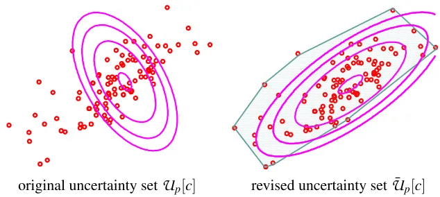
p[c]

Figure 3: Training samples and uncertainty sets. Left panel: original uncertainty set for the positive label. Right panel: revised uncertainty set consisting of the intersection of ellipsoid and convex-hull of input vectors with the positive label.

where b1and b2(>0)are constant numbers. Thus, we have

¯

U

o[c] =

∑

i∈Mo

αixi :

∑

i∈Mo

αi=1,αi≥0(i∈Mo),

∑

i∈Mo

α2

i ≤

c₋b1 mb2

=

z_∈conv_{xi:i∈Mo} :(z−x¯o)TbΣ−o1(z−x¯o)≤mo·

c₋b1 mb2

,

wherex¯oandΣboare the estimators of the mean vector and the covariance matrix for{xi:i∈Mo}.

The corresponding loss function is obtained in the same way as Example 4. Figure 3 illustrates an example of the revision of the uncertainty set. In the left panel, the uncertainty set does not match the distribution of the training samples. On the other hand, the revised uncertainty set in the right panel well approximates the dispersal of the training samples.

Example 6 Suppose that for o_{∈ {}p,n_},µois the mean vector andΣo is the covariance matrix of

the input vector conditioned on each label. We define the uncertainty set by

o_{∈ {}p,n_},

U

o[c] =

z_∈conv_{xi:i∈Mo}:(z−µ)TΣ−o1(z−µ)≤c,∀µ∈

A

,

where

A

denotes the estimation error of the mean vectorµ. For a fixed radius r>0,

A

is defined as

A

=µ_∈

X

: (µ₋µo)TΣ−o1(µ−µo)≤r2 .

The uncertainty set with the estimation error is used by Lanckriet et al. (2003) in MPM. The above uncertainty set is useful when the probability in the training phase is slightly different from that in the test phase. A brief calculation yields a representation of

U

o[c]in terms of the level set of the

convex function,

h∗_o(z) =max

µ∈A(z−µ)

T_Σ−1

o (z−µ) =

q

(z₋µo)TΣ−o1(z−µo) +r

The revised uncertainty set

U

¯o[c]is defined by the functionℓ¯∗:

¯

ℓ∗(α) =αmp

m −1 q µT

pΣ−p1µp+r

2 −

q µT

pΣ−p1µp+r

2

+αmn

m −1 q µT

nΣ−n1µn+r

2 −

q µT

nΣ−n1µn+r

2

. (23)

Suppose thatµp6=0andµn=0hold. Let d=

q µT

pΣ−p1µpand h=r/d(>0). The corresponding

loss function is

¯

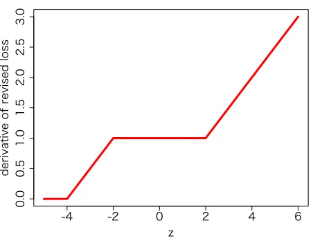
ℓ(z) =md 2 mp u z d2 ,

where u(z)as defined as

u(z) =             

0, z_{≤ −}2h₋2,

z

2+1+h

2

, ₋2h₋2_≤z_{≤ −}2h,

z+2h+1, ₋2h≤z≤2h, z2

4 +z(1−h) + (1+h)

2_{, 2h} ≤z.

(24)

Figure 4 depicts the function u(z) with h=1. When r =0 holds, ℓ¯(z) reduces to the truncated quadratic function shown in Example 4 and 5. For positive r,ℓ¯(z)is linear around z=0. This im-plies that by introducing the confidence set of the mean vector

A

, the penalty for the misclassification reduces from quadratic to linear around the decision boundary, though the original uncertainty set

U

o[c]does not correspond to minimization of an empirical loss function.

5. Kernel-Based Learning Algorithm Derived from Uncertainty Set

Suppose that we have training samples(x1,y1), . . . ,(xm,ym)∈

X

× {+1,−1}, where

X

is not nec-essarily a linear space. Let us define a kernel functionk:

X

2_{→R, and let}

_H

_{be the reproducing}

kernel Hilbert space (RKHS) endowed with the kernel functionk; see Sch¨olkopf and Smola (2002) for details about the kernel estimators in machine learning.

Let us start with the parametrized uncertainty sets

U

p[c]and

U

n[c] in

H

. Given uncertainty sets, a kernel variant of (16) is expressed as

inf cp,cn,fp,fn

cp+cn+λkfp−fnkH

subject to cp,cn∈R,

fp∈

U

p[cp]∩conv{k(·,xi):i∈Mp},

fn∈

U

n[cn]∩conv{k(·,xj): j∈Mn}.

(25)

Next, we find the corresponding loss functionℓ(z). Note that the revision of uncertainty sets pre-sented in Section 4 can be used, if necessary. Suppose the uncertainty sets are reprepre-sented as

U

o[c] =

∑

i∈Mo

αik(·,xi)∈

H

: 1

m_i∈

∑

_Moℓ ∗_(mα

i)≤c

[

SFWJTFEMPTT

MJOFBS

RVBESBUJD RVBESBUJD

Figure 4: Loss functionu(z)in Example 6 that corresponds to the revised uncertainty set with the estimation error.

foro_{∈ {}p,n_}. In the same way as in Section 3.1, we find that problem (25) is the dual representation of

min f,b,ρ−2ρ+

1

m

m

∑

i=1

ℓ(ρ₋yi(f(xi) +b))

subject to f _∈

H

,b_∈R_,ρ∈R_,kfk2

H ≤λ2.

(27)

We can obtain the estimated decision function fb+bb∈

H

+R by solving the problem (27). A rigorous proof of the strong duality between (25) and (27) is presented in Section 6 and Appendix B.

Example 7 (ellipsoidal uncertainty sets in RKHS) Let us consider an uncertainty set

U

[c]in RKHS

H

defined by

U

[c] = (_m

∑

i=1

αik(·,xi) : m

∑

i=1

α2

i ≤c

) ⊂

H

,

where x1, . . . ,xm are points in

X

. The corresponding loss is the truncated quadratic loss. Let us

definek¯_∈

H

as_m1∑mi=1k(·,xi). Furthermore, let us define the empirical variance operatorbΣ:

H

→

H

as

b

Σh= 1

m

m

∑

i=1

(k(_·,xi)−k¯)hk(·,xi)−k¯,hiH

for h∈

H

. Some calculation yields

U

[c]_∩conv_{k(_·,xi):i=1, . . . ,m}

=nk¯+bΣh :_hΣbh,h_{iH ≤}mc₋1o_∩conv_{k(_·,xi) :i=1, . . . ,m}.

By transforming the uncertainty-set-based learning into loss-based learning, we can obtain a statistical model for the conditional probability, as shown in Section 3.2. In addition, we can verify the statistical consistency of the learning algorithm with the (revised) uncertainty sets by taking the corresponding loss function into account. Other authors have proposed kernel-based learning algorithms with uncertainty sets (Lanckriet et al., 2003; Huang et al., 2004), but they did not deal with the issue of statistical consistency. In the following, we study the statistical properties of the learning algorithm based on (27).

6. Statistical Properties of Kernel-Based Learning Algorithms

Here, we prove that the expected 0-1 loss

E

(bf+bb)converges to the Bayes risk

E

∗defined by (1). We also determine whether certain popular uncertainty sets produce consistent learning methods. All proofs are presented in Appendix B and Appendix C.

6.1 Assumptions for Statistical Consistency

Let us show four assumptions.

Assumption 1 (universal kernel) The input space

X

is a compact metric space. The kernel func-tion k:

X

2_{→Ris continuous, and satisfies}

sup x_∈X

p

k(x,x)_≤K<∞,

where K is a positive constant. In addition, k is universal, that is, the RKHS associated with k is dense in the set of all continuous functions on

X

with respect to the supremum norm (Steinwart and Christmann, 2008, Definition 4.52).

Assumption 2 (non-deterministic assumption) For the probability distribution of training sam-ples, there exists a positive constantε>0such that

P(_{x_∈

X

:ε_≤P(+1_|x)_≤1₋ε_})>0,

where P(y_|x)is the conditional probability of the label y for the input x.

Assumption 3 (basic assumptions on loss functions) The loss functionℓ:R_→R_{satisfies the}

fol-lowing conditions.

1. ℓis a non-decreasing, convex function that is non-negative, that is,ℓ(z)_≥0for all z_∈R_.

2. Let∂ℓ(z)be the subdifferential of the loss functionℓat z_∈R_{(Rockafellar, 1970, Chapter 23).}

Then, the equalitylimz→∞∂ℓ(z) =∞holds; that is, for any M>0, there exists z0 such that g_≥M for all z_≥z0and all g∈∂ℓ(z).

Note that the second condition in Assumption 3 assures thatℓis not a constant function and that limz_→∞ℓ(z) =∞.

1. ℓ(z) is first order differentiable for z≥ −ℓ(0)/2, andℓ′_{(z)>0for z≥ −ℓ(0)/2, whereℓ}′ _is the derivative ofℓ.

2. Letψ(θ,ρ)be the function

ψ(θ,ρ) =ℓ(ρ)₋inf z∈R

1+θ

2 ℓ(ρ−z) + 1₋θ

2 ℓ(ρ+z)

, 0_≤θ_≤1,ρ_∈R_.

There exists a functionψe(θ)and a positive realε>0such that the following three conditions are satisfied:

(a) ψe(0) =0andψe(θ)>0for0<θ_≤ε.

(b) ψe(θ)is a continuous and strictly increasing function on the interval[0,ε].

(c) The inequalityψe(θ)_≤ inf

ρ≥−ℓ(0)/2ψ(θ,ρ)holds for0≤θ≤ε.

Appendix B presents a rigorous proof of the duality between (27) and (25) with the uncertainty set (26). Appendix C.3 presents sufficient conditions for the existence of the functionψein Assump-tion 4.

Under Assumptions 1–4 and another mild assumption, we prove that the expected 0-1 loss

E

(bf+bb) converges to the Bayes risk

E

∗_{. In the mild assumption, the covering number of the}

RKHS

H

is taken into account. The details of the conferring number are shown in Appendix C.1.

6.1.1 THEOREM(STATISTICALCONSISTENCY)

For the RKHS

H

and the loss functionℓ, we assume Assumptions 1, 2, 3 and 4. Also, we assume that

H

satisfies the covering number condition, that is,(41)in Appendix C.1 converges to zero for any positiveε, when the sample size m tends to infinity. Then,

E

(bf+bb)converges to

E

∗_{in probability.}

Appendix C presents the necessary definitions, lemmas, and theorems, and Theorem 8 of Ap-pendix C.1 and Theorem 9 of ApAp-pendix C.2 summarize the main results. The examples presented in Appendix C.3 show that some popular uncertainty sets and their revisions yield loss functions satisfying the above sufficient conditions.

6.2 Supplementary Explanations

Let us discuss Assumptions 1–4.

Universal kernel: The universality of RKHSs in Assumption 1 is usually assumed, when dis-cussing the statistical consistency of kernel methods. If the RKHS under consideration is not universal, a decision function might exist that is not approximated well by any element in the RKHS. The Gaussian kernel is universal, while the polynomial kernel is not universal.

Non-deterministic assumption: In Assumption 2, the labely is assigned in a non-deterministic way. The label assignment is deterministic when the conditional probabilityP(y= +1_|x)is equal to 0 or 1 for allx. Steinwart (2005) introduced they-degenerated condition defined as

for a labely∈ {+1,₋1_}. If they-degenerated condition holds, the proof of the consistency is straightforward for standard learning methods such asC-SVM. Involved mathematical ar-guments are needed to prove consistency if they-degenerated condition does not apply. Here, the deterministic assumption means

P(_{x_∈

X

:P(y_|x) =1 or 0_}) =1.

In our setup, the parameter ρ is a variable, and it makes the situation somewhat difficult. Under the above deterministic assumption, the optimal value of (27) may go to₋∞, as the number of training samples tends to infinity; see Lemma 3 in Appendix C.1. In such a case, it would be impossible to make an empirical approximation of the objective value in (27). We introduced the non-deterministic assumption to avoid such a troublesome situation.

Basic assumptions on loss functions: Loss functions are based on Assumption 3 and Assump-tion 4. CondiAssump-tions such thatℓ(z) is convex, non-decreasing, and bounded from below are standard ones, but the second condition in Assumption 3 is rather strong. The hinge loss and logistic loss do not satisfy this assumption, whereas the quadratic loss and exponential loss satisfy it. Assumption 3 is used to derive an upper bound of the optimalρin (27); see Lemma 5 in Appendix C.1.

Modified classification-calibrated loss: Assumption 4 is related to the classification-calibrated loss. Bartlett et al. (2006) introduced classification-calibrated losses to analyze the statis-tical consistency of binary classification problems. Roughly speaking, if a loss function is classification-calibrated, the minimizer of the loss function produces the minimizer of the 0-1 loss. See Bartlett et al. (2006) for details about classification-calibrated losses. Suppose that the functionℓ(ρ₋z)with a fixedρis convex inz_∈R_{. Then, a sufficient condition forℓ(}ρ₋z)

to be a classification-calibrated loss is given asℓ′(ρ)>0; that is,ℓis differentiable atρand the derivative is positive. In our setup, ρ is variable, and hence the conditionℓ′_{(ρ)>0 is}

required for all possible values ofρ. As shown in the proof of Lemma 5 in Appendix C.1, the optimalρof the problem (27) is bounded from below by₋ℓ(0)/2. Thus, we assumed the differentiability ofℓ(z)forz_{≥ −}ℓ(0)/2. The second condition of Assumption 4 defines the functions,ψ(θ,ρ)andψe(θ). Bartlett et al. (2006) defined the functionψ(θ,0) and derived the quantitative relation between the classification calibrated loss and the 0-1 loss viaψ(θ,0). We extendedψ(θ,0)toψ(θ,ρ)having a variableρ. The functionsψ(θ,ρ)andψe(θ)describe a qualitative relation between the convex lossℓand the 0-1 loss. Appendix C.2 uses the func-tionψe(θ)to prove that the convergence of the expected loss guarantees the convergence of the expected 0-1 loss to the Bayes risk.

7. Experiments

We conducted some numerical experiments to examine the prediction performance of our revision of uncertainty sets methods. The results indicate that the method improves the estimator. In addition, we evaluated the estimation accuracy of the conditional probability.

We compared the kernel-based learning algorithms using the Gaussian kernel. So far, many studies have compared linear models and kernel-based models. The conclusion is that linear models outperform kernel-based models when the linear models have good approximations of the deci-sion boundary. Otherwise, linear models have an approximation bias, and kernel-based estimators with a nice regularization outperform linear models. For this reason, we focused on kernel-based estimators.

The following methods were examined using the synthetic data and the standard benchmark data sets: C-SVM, MPM, unbiased MPM, and the learning method with (27). C-SVM is the one implemented in thekernlablibrary (Karatzoglou et al., 2004). In the unbiased MPM, the bias term

bof the model was estimated by minimizing the training error rate after estimating the function part,

b

f _∈

H

. The unbiased estimator will outperform the original MPM when the probability of the class label is heavily unbalanced. The loss functionℓ(z)of the proposed method was the functionu(z)in (24). This loss function corresponds to the revised uncertainty set of the ellipsoidal uncertainty set with the estimation error. The parameter in the functionu(z)of (24) was set toh=0 orh=1. The kernel parameter and the regularization parameter were estimated by 5-fold cross validation.

We evaluated the learning results as follows. We used the test error over the test samples to evaluate the classification accuracy. We assessed the estimation accuracies of the conditional prob-abilities given byC-SVM and the proposed method. AC-SVM with such a probability estimation is included in thekernlablibrary; the probability model is shown in Karatzoglou et al. (2004). We used the squared loss to assess the estimation accuracy of the conditional probability:

E

∑

y=±1

(Pb(y_|x)₋P(y_|x))2=E_Pb_(+1|x)2_+Pb_(−1|x)2₋₂E_Pb_(y|x) +E_P(+1|x)2_+P(−1|x)2_,

wherePb(y_|x)is an estimator of the true conditional probabilityP(y_|x). Since the last term of the above expression does not depend on the estimator, we used only the first two terms as the mea-sure of estimation accuracy. As a result, given test samples_{(_exi,eyi):ℓ=1, . . . ,L}, the estimated conditional probabilityPb(y_|x)can be approximately evaluated as follows:

squared-loss= 1

L

L

∑

ℓ=1

_b

P(+1_|exℓ)2+Pb(−1|exℓ)2− 2

L

L

∑

ℓ=1

b P(_eyℓ|exℓ).

This measure works even for benchmark data sets in which the true probability is unknown. Note that the squared-loss above can take negative values, since the last term in the expansion ofE_∑y=

±1(Pb(y|x)− P(y_|x))2_{is not taken into account. We did not use the Kullback-Leibler divergence or logarithmic}

loss, since the estimatorPb(y_|x)can take zero.

7.1 Synthetic Data

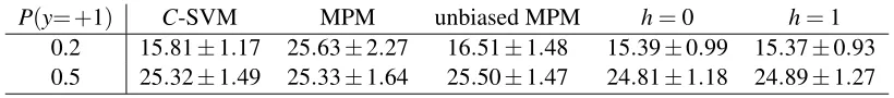
P(y= +1) C-SVM MPM unbiased MPM h=0 h=1 0.2 15.81_±1.17 25.63_±2.27 16.51_±1.48 15.39_±0.99 15.37_±0.93 0.5 25.32±1.49 25.33±1.64 25.50±1.47 24.81±1.18 24.89±1.27

Table 1: Test error (%) and standard deviation of each learning method. We comparedC-SVM, MPM, unbiased MPM, and the proposed learning method using the loss function (24) withh=0 orh=1.

matrix. The conditional distribution of the input points with the negative label was a normal dis-tribution with meanµn= (1,1)T and variance-covariance matrixΣn=RTdiag(0.52,1.52)R, where

Ris theπ/3 radian counterclockwise rotation matrix. The label probability wasP(y= +1) =0.2 or 0.5. The size of the training samples wasm=400. We computed test errors by averaging over 100 iterations. ForC-SVM and the proposed method, we computed the average squared-loss of the estimated conditional probability. We also evaluated average absolute difference between the true conditional probabilityP(+1_|x)and the estimatorPb(+1_|x) on the test set, that is, the average of

1

L∑ L

ℓ=1|P(+1|exℓ)−Pb(+1|exℓ)|over 100 iterations. This is possible, since the true probability of

synthetic data is known.

Table 1 shows the test errors ofC-SVM, MPM, unbiased MPM, and the proposed method using the loss function (24) withh=0 orh=1. The table shows that the MPM has an estimation bias for unbalanced samples, that is, the case ofP(y= +1) =0.2. MPM is slightly better than unbiased MPM on the setup of the balanced data. Overall, the proposed method is better than the other learning methods. Indeed, the difference between it andC-SVM is statistically significant. On the other hand, the parameterhin the loss function (24) does not significantly affect the experimental results.

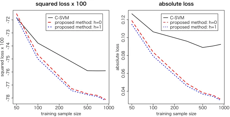
Table 2 shows the accuracy of the estimated conditional probabilities measured by the squared loss and absolute difference. As shown in the lower table, the absolute error of the proposed method is about 5%, while the error ofC-SVM is about 10%. The proposed method also outperformsC -SVM in terms of the squared-loss. C-SVM and the proposed method differ significantly in their estimation accuracy of the conditional probability, though the difference in classification error rate is less than 0.5%. Figure 5 presents the squared loss and absolute loss of the estimated conditional probability versus the size of the training samples forC-SVM and the proposed method withh=0 and h=1. The proposed method outperformsC-SVM. For each sample size, the parameter h

does not significantly affect the estimation accuracy, though the loss function u(z) withh=1 is consistently slightly better thanh=0.

7.2 Benchmark Data

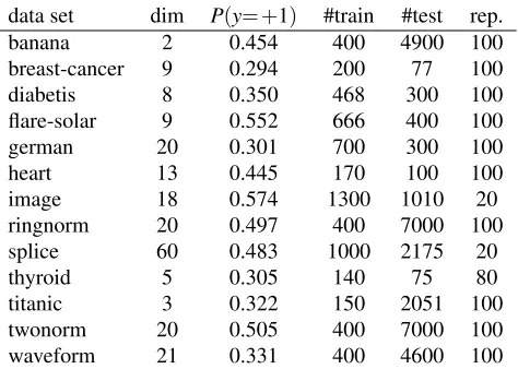
The experiments used thirteen artificial and real-world data sets from the UCI, DELVE, and STAT-LOG benchmark repositories: banana, breast-cancer, diabetes, german, heart, image,

squared-loss_×100

P(y= +1) C-SVM h=0 h=1 0.2 −75.43±1.78 −77.36±1.07 −77.42±1.08 0.5 ₋65.63_±1.89 ₋67.90_±1.07 ₋67.83_±1.21

absolute difference (%) betweenP(+1_|x)andPb(+1_|x)

P(y= +1) C-SVM h=0 h=1 0.2 9.37_±1.96 4.57_±1.28 4.43_±1.14 0.5 10.10_±2.34 5.11_±1.10 5.19_±1.32

Table 2: Squared loss and absolute loss of the estimated conditional probabilityPb(y_|x). We com-paredC-SVM and the proposed method using the loss function (24) withh=0 andh=1.

TRVBSFEMPTTY

USBJOJOHTBNQMFTJ[F

TRVBSFEMPTTY

$47.

QSPQPTFENFUIPEI QSPQPTFENFUIPEI

BCTPMVUFMPTT

USBJOJOHTBNQMFTJ[F

BCTPMVUFMPTT

$47.

QSPQPTFENFUIPEI QSPQPTFENFUIPEI

Figure 5: Squared loss and absolute loss of estimated conditional probability versus training sample size are presented forC-SVM and the proposed method withh=0 andh=1.

replications of learning to evaluate the average performance. Table 4 shows the test errors(%)and the standard deviation for the benchmark data sets.

data set dim P(y= +1) #train #test rep.

banana 2 0.454 400 4900 100

breast-cancer 9 0.294 200 77 100

diabetis 8 0.350 468 300 100

flare-solar 9 0.552 666 400 100

german 20 0.301 700 300 100

heart 13 0.445 170 100 100

image 18 0.574 1300 1010 20

ringnorm 20 0.497 400 7000 100

splice 60 0.483 1000 2175 20

thyroid 5 0.305 140 75 80

titanic 3 0.322 150 2051 100

twonorm 20 0.505 400 7000 100

waveform 21 0.331 400 4600 100

Table 3: The properties of each data sets: “dim”, “P(y= +1)”,“#train”, “#test” and “rep.” respec-tively denote the input dimension, the ratio of the positive label in the training samples, the size of the training set, the size of the test set, and the number of replications of learning.

The boldface letters in Table 4 indicate the smallest average test error for each data set. Over-all,C-SVM and the learning method “h=1” outperform the others.C-SVM is significantly better than the proposed method with “h=1” onflare-solar, ringnorm andtwonorm, but the pro-posed method with “h=1” is significantly better thanC-SVM onbanana,diabetis,germanand

waveform. These results show that the proposed method with “h=1” is comparable toC-SVM. Table 5 shows the squared-losses for estimated conditional probabilities. It shows that the proposed method with “h=1” outperforms the others in the conditional probability estimation.

In Section 6, we proved the statistical consistency of learning methods derived from the un-certainty set approach. The numerical experiments described in this section indicate that learning methods derived from revised uncertainty sets are an alternative for solving classification problems involving conditional probability estimations.

8. Conclusion