Evolving Static Representations for Task Transfer

Evolving Static Representations for Task Transfer

Phillip Verbancsics [email protected]

Kenneth O. Stanley [email protected]

School of Electrical Engineering and Computer Science University of Central Florida

Orlando, FL 32816, USA

Editor: Michael Littman

Keywords: transfer learning, task transfer, evolutionary computation, neuroevolution, indirect encoding

Abstract

An important goal for machine learning is to transfer knowledge between tasks. For example, learn-ing to play RoboCup Keepaway should contribute to learnlearn-ing the full game of RoboCup soccer. Previous approaches to transfer in Keepaway have focused on transforming the original represen-tation to fit the new task. In contrast, this paper explores the idea that transfer is most effective if the representation is designed to be the same even across different tasks. To demonstrate this point, a bird’s eye view (BEV) representation is introduced that can represent different tasks on the same two-dimensional map. For example, both the 3 vs. 2 and 4 vs. 3 Keepaway tasks can be represented on the same BEV. Yet the problem is that a raw two-dimensional map is high-dimensional and un-structured. This paper shows how this problem is addressed naturally by an idea from evolutionary computation called indirect encoding, which compresses the representation by exploiting its geom-etry. The result is that the BEV learns a Keepaway policy that transfers without further learning or manipulation. It also facilitates transferring knowledge learned in a different domain, Knight Joust, into Keepaway. Finally, the indirect encoding of the BEV means that its geometry can be changed without altering the solution. Thus static representations facilitate several kinds of transfer.

1. Introduction

capabilities within the new scenario. As an alternative, this paper argues that an ideal representation would require no such transformations (i.e., it would remain static) when transferring to a new task. The idea that input (i.e., state) representation might remain static during transfer is plausible because the raw inputs to biological organisms, for example, vision, remain the same even when new tasks are confronted. For example, when a child graduates from playing Keepaway to full-blown soccer, the number of photoreceptors in the eye do not change. The main idea in this paper is that such static representation, when possible, facilitates transfer by ensuring that the semantics of the representation are preserved even when the task changes.

To demonstrate the critical role of static representation in transfer, a novel state representation is introduced called a bird’s eye view (BEV), which is a two-dimensional depiction of objects on the ground from above. Conceptually, the BEV is a metaphor for an internal representation of the state of the world from above. The BEV places objects into the context of the world geometry, allowing geometric relationships to be more easily learned. Another advantage is that its input dimensionality (i.e., number of inputs) is constant no matter how many objects are on the field. That way, even if the task is transferred to a version with more objects, the representation remains the same (i.e., static), significantly simplifying task transfer.

However, the challenge for the BEV is that representing a high-resolution two-dimensional field requires many input dimensions (i.e., many parameters), similarly to an eye. An outgrowth of evolutionary computation designed to address such high-dimensional problems is indirect en-coding, which compresses the representation of the solution by reusing information. The particular indirect encoding in this paper, called a compositional pattern producing network (CPPN; Stan-ley 2007), represents artificial neural network (ANN) mappings between high-dimensional spaces by exploiting regularities in their geometry, which is well-suited to the BEV. An evolutionary al-gorithm called Hypercube-based NeuroEvolution of Augmenting Topologies (HyperNEAT; Gauci and Stanley 2008; Stanley et al. 2009; Gauci and Stanley 2010) that is designed to evolve CPPNs is therefore able to learn effectively from the BEV.

The HyperNEAT BEV is tested in the common RoboCup Keepaway soccer reinforcement-learning (RL) benchmark (Stone et al., 2005). Keepaway is important because it can potentially serve as a stepping stone to full-blown soccer in the future, which is a major current goal in machine learning (Kalyanakrishnan et al., 2007; Kitano et al., 1997; Kok et al., 2005; Kyrylov et al., 2005; Mackworth, 2009; Stolzenburg et al., 2006). One interesting result with the BEV is the longest holding time in the 3 vs. 2 variant of the task yet recorded. However, more importantly, unlike any method so far, HyperNEAT can transfer from 3 vs. 2 to 4 vs. 3 Keepaway with no change in representation and no further learning, demonstrating the critical role static representation plays in learning and transfer. Furthermore, these transferred policies can then be further trained on the new task without the need to alter the representation. Additional types of transfer within Keepaway are investigated wherein the representation of the policy (i.e., the CPPN, or indirect encoding) remains static while the BEV itself is changed by increasing resolution and by accommodating different field sizes. Finally, cross-domain transfer is demonstrated by training on a distinctly different do-main, Knight Joust (Taylor et al., 2007a), which is a simple predator-prey type dodo-main, and then transferring to 3 vs. 2 Keepaway.

learning often focuses on the learning algorithm, the hope is that this paper provokes a fruitful conversation on the role of representation in transfer and learning in general.

It is finally important to acknowledge that the extent to which maintaining a static representation is realistic depends upon the learning method, state information, and differences between domains. Thus static representation is an ideal that when met can provide an advantage, as shown in this paper.

The next section describes the importance of representation in learning, prior research in transfer learning, and the methods that underlie the BEV representation. Section 3 explains how the BEV is configured, how information is represented in the BEV, and how HyperNEAT trains the BEV. In Section 4, the experiments that investigate the performance of the BEV in learning and transfer are described. Finally, Section 5 presents the results of the BEV, followed by a discussion in Section 6.

2. Background

This section examines the critical role of representation in RL and then explains the geometry-based methods that underlie the static representation investigated in this paper, and their relation to task transfer.

2.1 Representation in Learning

A convenient model for problems in RL is the Markov decision process (MDP). In the MDP, the learner knows its environment through a state observation s∈S, which is characterized by a set of state variables s=hp1,p2,· · ·,pni, in which each pi denotes a particular state parameter. By taking an action a∈A, the agent transitions to a new state in S through the transition function T : S×A7→S. The reward function R : S7→Rdetermines the instantaneous reward associated with reaching each state. Finally, the action that the agent takes from its current state is selected by the policy function

π: S7→A (Puterman, 1994). For example, in the Keepaway soccer domain, the state space S for the keeper with the ball can be defined as the set of distances and angles to each other player. The set of actions A can be defined as a set of passes to teammates and holding the ball (Metzen et al., 2007; Stone et al., 2001; Stone and Sutton, 2001; Stone et al., 2005). A simple policyπwould be to pass to the most open teammate when takers are close and hold the ball otherwise.

While the MDP framework provides a solid foundation for developing learning algorithms, it does not suggest how to select a state and action representation appropriate for both the domain and the learning algorithm. One popular approach to state representation, for example, in the RoboCup Keepaway soccer domain, is to express the state as distances and angles to the other players rela-tive to the agent with the ball (Metzen et al., 2007; Stone et al., 2001, 2005; Taylor et al., 2006). However, this common representation is not the only one possible, which is important because repre-sentation critically influences what is learned (Gauci and Stanley, 2008; Diuk et al., 2008; Tadepalli et al., 2004; Tesauro, 1992).

be learned repeatedly when the same decisions are made separately for multiple objects, such as whether to pass to teammates who are out of bounds.

Relational RL addresses problems such as scaling and repetitious concepts by generalizing the representation of information for learning algorithms to a relational form (Deroski et al., 2001). For example, in the RoboCup Keepaway domain, instead of real-valued state parameters, general relations can be defined. An example for deciding to whom to pass in 3 vs. 2 Keepaway is:

Pass(Teammate):−T hreatened(PlayerWithBall),Open(Teammate).

The relational form provides a more expressive representation that can be combined with reinforcement-learning methods (Tadepalli et al., 2004). By focusing on the logic of relationships, instead of on individual parameter values, these relationships can be applied to any number of ob-jects. Furthermore, once a relationship is learned for one set of objects, it is learned for all similar sets of objects.

One of relational RL’s goals is to provide an easier representation for transferring knowledge. This transfer could be across objects in the domain or across different tasks. However, the design and definition of these relationships are dependent upon the human designer, requiring expert do-main knowledge. Learning is dependent upon the a priori defined relations. Continuous and noisy domains present additional challenges to designing appropriate relations (Morales, 2003). Never-theless, relational RL highlights the importance of representation to learning.

However, while state representation is important, it is not the only type of representation that affects learning. Also significant is the representation of the learner itself, which impacts which types of relationships can be learned and how easily they are found. For example, research in temporal difference learning can employ look-up tables or more compact representations (Sutton, 1988, 1996; Tesauro, 1992), which work by encoding regularities. An important difference between these representations is that the look-up table contains enough parameters to store associated actions with every state, while compact representations must encode the solution with significantly fewer parameters than states. To guarantee convergence with a look-up table, every state must be visited an infinite number of times (Sutton and Barto, 1998) while compact representations need only discover underlying regularities in the problem (Sutton, 1996; Tesauro, 1992).

Another important factor in representation is the geometry of the domain (e.g., which position is adjacent to which and in what direction). Geometry plays a critical role in learning. For example, if a checkers board is scrambled while the relationships among locations that have been moved remain the same, the game would become more difficult to learn. This effect has been investigated in checkers, wherein learning based on board geometry was demonstrated to enhance performance versus learning while blind to geometry (Gauci and Stanley, 2008, 2010). Ideally, the solution should be a function of the domain geometry, enabling the learner to take advantage of geometric regularities. This paper focuses further on the critical role of representing geometry, particularly in task transfer, which is described next.

2.2 Task Transfer

1997; Schmidhuber and Informatik, 1994; Tadepalli, 2008; Thrun and Mitchell, 1994). Thus the capability to transfer is becoming increasingly important as the tasks studied in RL increase in complexity. However, transfer learning faces several challenges: First, transfer is only effective among compatible tasks and the particular knowledge that can transfer from one task to another must be identified. Second, a method must be derived to actually implement the transfer of knowledge. Finally, cases in which transfer hinders performance, or negative transfer, must be avoided (Pan and Yang, 2008). There are several types of transfer learning problems and a variety of methods that exploit their characteristics. These methods include translating the knowledge learned in one task to another task (Ramon et al., 2007; Taylor et al., 2007a), choosing the best policy for the current task from a set of previously learned policies (Talvitie and Singh, 2007), extracting advice from previously learned tasks (Torrey et al., 2008a,b), and learning multiple tasks at the same time (Collobert and Weston, 2008). This section reviews several such approaches.

An intuitive approach to transfer learning is to transform the representation of knowledge learned in one task to a suitable form for a new task and then continue learning from that point. A success-ful method that takes this approach is transfer via inter-task mapping for policy search methods (TVITM-PS; Taylor et al. 2007a). TVITM-PS is such a leading method for transforming the policy learned in the source task into a policy usable in the target task. In TVITM-PS, a transfer func-tionalρis defined to transform the policyπfor a source task into the policy for a target task, such thatρ(πsource) =πtarget. This functional is often hand-coded based on domain knowledge, though learning it is possible. When there are novel state variables or actions, an incomplete mapping is defined from the source to the target. TVITM-PS can be adapted to multiple representations. For example, in an ANN, input or output nodes whose connections are not defined in the mapping (i.e., it is incomplete) are made fully connected to the existing hidden nodes with random weights. This incomplete mapping implies that further training is needed to optimize the policies with respect to the new state variables and actions. However, it makes it possible to begin in the target domain from a better starting point than from scratch. TVITM-PS is a milestone in task transfer because it introduces a formal approach to moving from one domain to another that defines how ambiguous variables in the target domain should be treated. The performance of TVITM-PS is compared to results in this paper.

allows an accurate estimate of which policy from previously learned tasks is appropriate for the cur-rent task. In contrast to this approach, this paper focuses on how to effectively leverage knowledge gained in a single source policy to continue learning in the target domain. Thus the approach in this paper can potentially combine with a multi-policy approach such as AtEase.

An important consideration in transfer is whether a human can understand the knowledge being transferred among tasks. An alternative method to recycling previously learned policies directly is to take advice from learned policies to augment decision making. This advice may take the form of geometric knowledge, causal relationships, predictions, or any other type of information, allowing researchers to more easily interpret the transferred knowledge. Rule extraction is one such method that takes knowledge learned from a source domain and translates it into advice that aids a policy in a target domain (Torrey et al., 2008b). The advice is generated as a conditional, if-then statement. Torrey et al. (2008b) describe two methods for generating advice. One method is to compose rules by decomposing the policy learned on a source task. For example, Q-values can be examined directly and rules can be generated based on which actions are preferred. An alternative method for generating advice is to analyze the behavior (instead of the policy) of an agent to generate rules. Consider observing agents playing a game of Keepaway soccer. Through observation, it may be apparent that a learned policy always passes the ball if opponents approach within one meter, which may then be transformed into a rule to transfer to another task. These sets of rules have the advantage of being understandable to humans, allowing researchers to know what knowledge is being transferred and how it is contributing.

Interestingly, transfer learning does not always require a designated source and target task. In-stead, knowledge may transfer among several tasks that are simultaneously being learned. By en-coding the knowledge for multiple tasks within the same policy, the knowledge gained from each individual task may combine with and complement the knowledge from other tasks. For example, Collobert and Weston (2008) demonstrate transfer learning through multi-task training for natu-ral language processing (NLP) with deep neunatu-ral networks. There are many tasks related to NLP, including part-of-speech tagging, chunking, named entity recognition, semantic role labeling, lan-guage modeling, and relating words syntactically. The idea is that learning about one such task may contribute to learning the others. By training the policies simultaneously for all these capabilities, knowledge can be continually passed back and forth among all these tasks. In particular, Collobert and Weston (2008) show that this method improves generalization and achieves competitive results on the task of relating words with similar meaning.

This paper adds to our understanding of task transfer by focusing on the role of representation. The next section reviews the NEAT method, upon which this representation-centric approach is built.

2.3 NeuroEvolution of Augmenting Topologies (NEAT)

NEAT is an evolutionary algorithm that starts with a population of small, simple ANNs that increase their complexity over generations by adding new nodes and connections through mutation. That way, the topology of the network does not need to be known a priori and NEAT finds a suitable level of complexity for the task. NEAT is unlike many previous methods that evolved neural net-works, that is, neuroevolution methods, which historically evolved either fixed-topology networks (Gomez and Miikkulainen, 1999; Saravanan and Fogel, 1995), or arbitrary random-topology net-works (Angeline et al., 1993; Gruau et al., 1996; Yao, 1999). Unlike these approaches, NEAT begins evolution with a population of small, simple networks and increases the complexity of the network topology into diverse species over generations, leading to increasingly sophisticated behavior. A similar process of gradually adding new genes has been confirmed in natural evolution (Martin, 1999; Watson et al., 1987) and shown to improve adaptation in a few prior evolutionary (Altenberg, 1994) and neuroevolutionary (Harvey, 1993) approaches. However, a key feature that distinguishes NEAT from prior work in growing ANNs is its unique approach to maintaining a healthy diversity of increasingly complex structures simultaneously, as this section reviews. Complete descriptions of the NEAT method, including experiments confirming the contributions of its components, are available in Stanley and Miikkulainen (2002, 2004) and Stanley et al. (2005).

The NEAT method is based on three key ideas. First, to allow network structures to increase in complexity over generations, a method is needed to keep track of which gene is which. Otherwise, it is not clear in later generations which individual is compatible with which in a population of diverse structures, or how their genes should be combined to produce offspring. NEAT solves this prob-lem by assigning a unique historical marking to every new piece of network structure that appears through a structural mutation. The historical marking is a number assigned to each gene corre-sponding to its order of appearance over the course of evolution. The numbers are inherited during crossover unchanged, and allow NEAT to perform crossover among diverse topologies without the need for expensive topological analysis.

Second, NEAT divides the population into species so that individuals compete primarily within their own niches instead of with the population at large. Because adding new structure is often initially disadvantageous, this separation means that unique topological innovations are protected and therefore have the opportunity to optimize their structure without direct competition from other niches in the population. The historical markings help NEAT determine to which species different individuals belong.

Third, many approaches that evolve network topologies and weights begin evolution with a population of random topologies (Gruau et al., 1996; Yao, 1999). In contrast, NEAT begins with a uniform population of simple networks with no hidden nodes, differing only in their initial random weights. Because of speciation, novel topologies gradually accumulate over evolution, thereby al-lowing diverse and complex phenotype topologies to be represented. No limit is placed on the size to which topologies can grow. New structures are introduced incrementally as structural mutations occur, and only those structures survive that are found to be beneficial through fitness evaluations. In effect, then, NEAT searches for a compact, appropriate topology by incrementally adding com-plexity to existing structure.

2.4 CPPNs and HyperNEAT

The primary reason that NEAT is chosen as the main vehicle to study alternate representations is that it is easily extended to become an indirect encoding, which means a compressed description of the solution network. Such compression makes the policy search practical even if the state space is high-dimensional. One effective approach to indirect encoding is to compute the network structure as a function of the domain’s geometry. This section describes such an extension of NEAT, called Hypercube-based NEAT (HyperNEAT; Gauci and Stanley 2008; Stanley et al. 2009; Gauci and Stanley 2010), which enables the novel state representation in this paper from a bird’s eye view. The effectiveness of the geometry-based learning in HyperNEAT has been demonstrated in multiple domains, such as checkers (Gauci and Stanley, 2008, 2010), multi-agent predator prey (D’Ambrosio and Stanley, 2008; D’Ambroiso and Stanley, 2010), visual discrimination (Stanley et al., 2009), and quadruped locomotion (Clune et al., 2009). For a full HyperNEAT description, see Stanley et al. (2009) and Gauci and Stanley (2010).

The main idea in HyperNEAT is that it is possible to learn geometric relationships in the domain through an indirect encoding that describes how the connectivity of the ANN can be generated as a function of the domain geometry. Unlike a direct representation, wherein every dimension in the policy space (i.e., each connection in the ANN) is described individually, an indirect representation can describe a pattern of parameters in the policy space without explicitly enumerating every such parameter. That is, information is reused in such an encoding, which is a major focus in the field of generative and developmental systems from which HyperNEAT originates (Bentley and Kumar, 1999; Hornby and Pollack, 2002; Lindenmayer, 1968; Turing, 1952). Such information reuse is what allows indirect encodings to search a compressed space. That is, HyperNEAT discovers the regularities in the domain geometry and learns a policy based on them.

The indirect encoding in HyperNEAT is called a compositional pattern producing network (CPPN; Stanley 2007), which encodes the connectivity pattern of an ANN (Gauci and Stanley, 2007, 2008; Stanley et al., 2009; Gauci and Stanley, 2010). The idea behind CPPNs is that a ge-ometric pattern can be encoded by a composition of functions that are chosen to represent several common regularities. For example, because the Gaussian function is symmetric, when it is com-posed with any other function, the result is a symmetric pattern. The internal structure of a CPPN is a weighted network, similar to an ANN, that denotes which functions are composed and in what order. The appeal of this encoding is that it can represent a pattern of connectivity, with regularities such as symmetry, repetition, and repetition with variation, through a network of simple functions (i.e., the CPPN), which means that, instead of evolving ANNs directly, NEAT can evolve CPPNs that generate ANN connectivity patterns (Figure 1). Furthermore, the indirect encoding represents the connectivity of the ANN regardless of its size, which allows ANNs of arbitrary dimensionality to be represented.

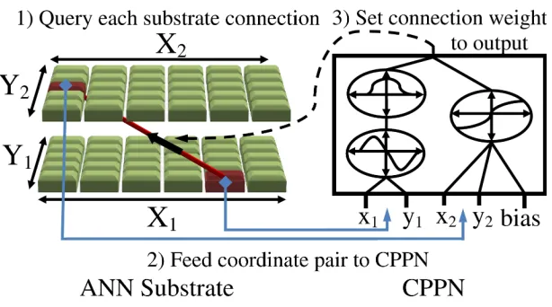
Figure 1: A CPPN Describes Connectivity. A grid of nodes, called the ANN substrate, is assigned coordinates. (1) Every connection between layers in the substrate is queried by the CPPN to determine its weight; the line connecting layers in the substrate represents a sample such connection. (2) For each such query, the CPPN inputs the coordinates of the two endpoints, which are highlighted on the input and output layers of the substrate. (3) The weight between them is output by the CPPN. Thus, CPPNs, whose internal topology and connection weights are evolved by HyperNEAT, can generate regular patterns of connections.

every pair of points in the space, the CPPN can produce an ANN, wherein each queried point is the position of a neuron. While CPPNs are themselves networks, the distinction in terminology between CPPN and ANN is important for explicative purposes because in HyperNEAT, CPPNs en-code ANNs. Because the connection weights are produced as a function of their endpoints, the final structure is produced with knowledge of the domain geometry, which is literally depicted geometri-cally within the constellation of nodes. In other words, parameters piof the state vector s actually exist at coordinates in space, giving it a geometry.

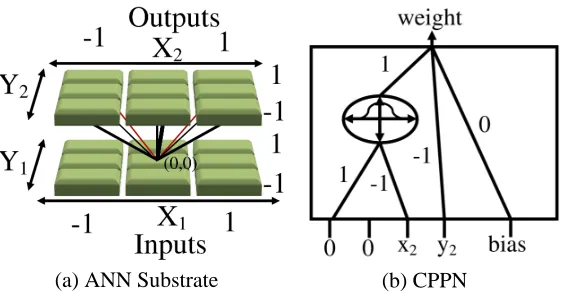
To help explain how CPPNs can compactly encode regular connectivity patterns, Figure 2 shows how a very simple CPPN encodes a symmetric network. In effect, the CPPN paints a pattern within a four-dimensional hypercube that is interpreted as an isomorphic connectivity pattern. The example in Figure 2 illustrates the natural connection between the function embodied by the CPPN and the geometry of the resultant network.

(a) ANN Substrate (b) CPPN

Figure 2: Example CPPN Describing Connections from a Single Node. An example CPPN (b) with five inputs(x1,y1,x2,y2,bias) and one output (weight) contains a single Gaussian node and five connections. The function produced is symmetric about x1and x2(because of the Gaussian) and linear with respect to y2(which directly connects to the CPPN output). For the given fixed input node coordinate(x1=0,y1=0), the CPPN in effect produces the function Gaussian(−x2)−y2. This pattern of weights from input node(0,0)is shown on the substrate (a). Weight magnitudes are indicated by thickness and black lines indicate positive values. Note that the pattern produces a set of weights that are symmetric about the x-axis and linearly decreasing as the values of y2increases. In this way, the function embodied by the CPPN encodes a geometric pattern of weights in space. HyperNEAT evolves the topologies and weights of such CPPNs.

or symmetry, which the CPPN sees) of a problem that are invisible to traditional encodings. For example, one way that geometric knowledge can be imparted is by including a hidden node in the CPPN that computes Gaussian(x2−x1), which imparts the concept of locality on the x-axis, an idea employed in the implementation in this paper. The HyperNEAT algorithm is outlined in algorithm 1.

In summary, instead of evolving the ANN directly, HyperNEAT, through the NEAT method, evolves the internal topology and weights of the CPPN that encodes it, which is significantly more compact. The next section explains how this encoding makes it possible to learn from a bird’s eye view.

3. Approach: Bird’s Eye View

Input: Substrate Configuration Output: Solution CPPN

Initialize population of minimal CPPNs with random weights; 1

while Stopping criteria is not met do 2

foreach CPPN in the population do 3

foreach Possible connection in the substrate do 4

Query the CPPN for weight w of connection; 5

if Abs(w)>Threshold then 6

Create connection with a weight scaled proportionally to w (Figure 1); 7

end 8

end 9

Run the substrate as an ANN in the task domain to ascertain fitness; 10

end 11

Reproduce CPPNs according to the NEAT method to produce the next generation; 12

end 13

Output the Champion CPPN. 14

Algorithm 1: Basic HyperNEAT Algorithm

3.1 Bird’s Eye View

Humans often visualize data from a BEV. Examples include maps for navigation, construction blue prints, and sports play books. Key to these representations is that they remain the same (i.e., they are static) no matter how many objects are represented on them. For example, a city map does not change size or format when new buildings are constructed or new roads are created. Addition-ally, the physical geometry of such representations allow agents to understand spatial relationships among objects in the environment by placing them in the context of physical space. The BEV also implicitly represents its borders by excluding space outside them from its field of view. As sug-gested in Kuipers’ Spatial Semantic Hierarchy (SSH), such metrical representation of the geometry of large-scale space is a critical component of human spatial reasoning (Kuipers, 2000).

A distinctive feature of the proposed representation is that not only is the agent state represented from a BEV, but it also requests actions within the same BEV perspective. For example, to request a pass the agent can indicate its target by simply highlighting it on a two-dimensional output array. That way, instead of making decisions blind to the geometry of physical space, it can be taken into account.

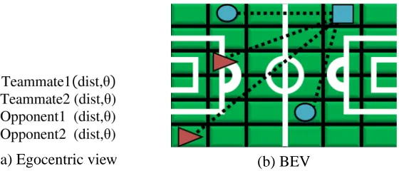
Egocentric data (Figure 3a) can be mapped to an equivalent BEV by translating from local (relative) coordinates to global coordinates established by static points of reference (i.e., fiducials). The global coordinates mark the location of objects in the BEV (Figure 3b). This translation allows mapping any number of objects into the static representation of the BEV.

Importantly, the continuous coordinate system must be discretized so that each variable in the state representation corresponds to a single discrete location. This discretization allows the two-dimensional field to be represented with a finite set of parameters. The values of these parameters denote objects in their respective regions.

(a) Egocentric view (b) BEV

Figure 3: Alternative Representations of a Soccer Field. Several parameters (a) represent the agent’s relationship with other agents on a soccer field (taken from a standard RoboCup representation; Cheny et al. 2003). Each distance and angle pair represents a specific relationship of the agent to another agent. The BEV (b) represents the same relationships as paths in the geometric space. A square depicts the agent, circles depicts its teammates, and triangles its opponents. The overhead perspective also makes it possible to represent any number of agents without changing the representation.

would still be egocentric whereas the BEV is not, and (2) tile coding breaks the state representation into chunks that can be optimized separately whereas the HyperNEAT CPPN derives the connectiv-ity of the policy network directly from the geometric relationships among the squares in Figure 3b, as explained next.

3.2 HyperNEAT: Learning from the BEV

Geometric patterns often exhibit spatial regularities. Examples include repetition and symmetry. Furthermore, important geometric relationships such as locality and topological connectedness of-ten critically influence informed spatial decision-making. The challenge for machine learning is that learning is often blind to the geometry of the problem, making it difficult to exploit such relation-ships (Gauci and Stanley, 2008, 2010). To understand the impact of learning from the true geometry of the domain, consider a two-dimensional field converted to a traditional vector of parameters, which removes the geometry (Figure 4). For example, consider a set of input values to an ANN such as in to Figure 3a. Though each dist andθpair is critically related in such a traditional rep-resentation, an ANN has no inherent knowledge or explicit access to this relationship. In contrast, HyperNEAT sees the task geometry, thereby exploiting geometric regularities and relationships, such as locality, which the BEV naturally makes explicit.

con-Figure 4: The Importance of True Geometry. A two-dimensional field transformed into a vector of parameters without any geometry forfeits knowledge of the geometry of the domain.

nections between regions in the physical space. To represent world state, objects and agents are literally “drawn” onto the input substrate, which is a static size, like marking a map. The generated network then can make decisions based on the relationships of such features in physical space and thereby learn the significance of certain kinds of geometric relationships among objects that are not identified a priori by the designer.

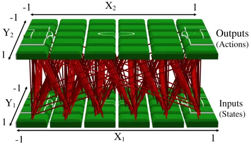
Figure 5: BEV Implemented in the Substrate. Each dimension ranges between[−1,1]and the input and output planes of the substrate are equivalently constructed to take advantage of geo-metric regularities between states and actions. Because CPPNs are an indirect encoding, the high dimensionality of the weights does not affect performance. (The CPPN is the search space.)

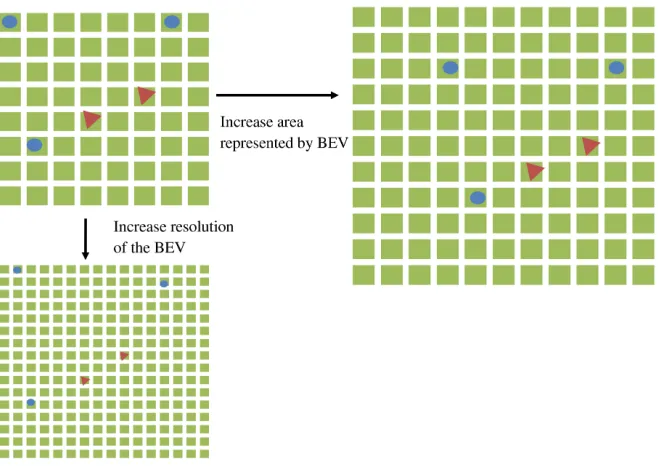
Interestingly, although the BEV is naturally held static its size or resolution can be changed without retraining. A unique feature of CPPNs (which encode the BEV connectivity) is that the same CPPN can query substrates of arbitrary size or resolution. It is important to note that even when size or resolution are changed, the CPPN itself remains the same. Thus the BEV can extend its representation to different field sizes or to different levels of detail (i.e., resolutions), as shown in Figure 6. In this way, the CPPN allows not only transfer to different numbers of players, but to different field sizes and resolutions, all without the need for retraining.

Figure 6: Changing the BEV. Two kinds of alterations are depicted in this figure. First, the BEV can be altered by increasing the area of the substrate while maintaining the size of each discrete cell by extrapolating new connection weights associated with previously unseen cells. Second, resolution is increased by increasing the number of cells and shrinking the area represented by each discrete cell. The CPPN automatically interpolates connection weights for the new locations. Thus, the BEV allows new forms of transfer to differing field sizes or levels of precision.

new connections automatically. Although the number of connections in this example increases from 160,000 to 2,560,000, the dimensionality of the CPPN does not change at all.

The next section introduces the experiments that demonstrate the benefits of this geometric approach.

4. Experimental Setup

The experiments in this paper are designed to investigate the role of representation in task transfer. Of course, some representations are better suited to transfer in a given domain than others. Further, the ability to transfer between tasks is dependent on the similarity of the tasks. However, this paper focuses on the idea that a particularly effective representation for transfer is one that does not need to change from one task to the next. Because the representation is consistent, it has the potential to exhibit improved performance in the target domain immediately after transfer, without further learning. The advantage of a consistent representation is that the semantic relationships learned previously are preserved and then can be built upon. Because the BEV is the same irrespective of the number of players on either side, it satisfies this requirement and allows the hypothesis that consistent representation leads to immediate improvement in the target domain to be tested. This section explains the domains, the methods compared, and the experimental configurations.

4.1 RoboCup Keepaway Domain

RoboCup simulated soccer Keepaway (Stone et al., 2001) is well-suited to such an investigation because it is a popular RL performance benchmark and can be scaled to different numbers of agents to create new versions of the same task. All experiments are run on the Keepaway 0.6 player bench-mark (Stone et al., 2006) and the RoboCup Simulator Soccer Server v. 12.1.1 (Cheny et al., 2003). RoboCup Keepaway is a popular benchmark (Metzen et al., 2007; Stone et al., 2005; Taylor et al., 2007a; Whiteson et al., 2005) in part because it includes a large state space, partially observable state, and noisy sensors and actuators. It is also a stepping stone to full-blown RoboCup Soccer, one of the hottest tasks in machine learning (Kalyanakrishnan et al., 2007; Kitano et al., 1997; Kok et al., 2005; Kyrylov et al., 2005; Mackworth, 2009; Stolzenburg et al., 2006). In Keepaway, keep-ers try to maintain possession of the ball within a fixed region and takkeep-ers attempt to take it away. The number of agents and size of the field can be varied to make the task more or less difficult: The smaller the field and the more players in the game, the harder it becomes.

4.2 Keepaway Benchmark

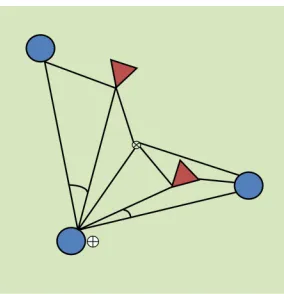
Figure 7: Visualization of Traditional State Variables in 3 vs. 2 Keepaway. The 13 state parameters that represent the state in the 3 vs. 2 Keepaway task are depicted in this figure. The three keepers are represented by the circles and the takers represented by the triangles. The state parameters include the distances from each player to the center of the field (marked by the circle with the ×), the distances from the keeper with the ball (denoted by the circle with the +) to each other player, the distance from each other keeper to the taker nearest them, and the angles along the passing lanes.

To investigate the ability of a static representation, that is, the HyperNEAT BEV, to learn this task, it is compared to both static policies (Stone et al., 2006) and the learning algorithms Sarsa (Rummery and Niranjan, 1994), NEAT (Stanley and Miikkulainen, 2004), and EANT (Metzen et al., 2007). Unlike the BEV, the traditional representation (with 13 state variables) through which these methods learn in 3 vs. 2 Keepaway must be changed for different versions of the task, such as 4 vs. 3 Keepaway. The static benchmarks are Always-Hold, Random, and a Hand-Coded policy, which holds the ball if no takers are within 10m (Stone and Sutton, 2001). These static benchmarks provide a baseline to validate that the BEV learns a non-trivial policy in the initial task.

State action reward state action (Sarsa; Rummery and Niranjan 1994) is an on-policy temporal difference RL method that learns the action-value function Q(s,a). The quintuple (s,a,r,s′,a′)

defines the update function for Q(s,a)by determining for a current state (s) and action (a) what the reward (r) and the expected reward for the predicted next state (s′) and action (a′) will be. The update equation is:

Q(s,a)←(1−α)Q(s,a) +α(r+γQ(s′,a′)),

whereαis the learning rate andγis the discount factor for the future reward. The values in Q(s,a)

determine which action is taken in a given state by selecting the maximal value. Each keeper separately learns which action to take in a given state to maximize the reward it receives (Taylor et al., 2006).

during the evolutionary process. These methods were chosen for comparison because they have been tested in the same Keepaway configuration.

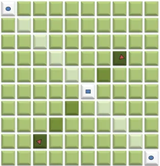
As described in Section 3, the HyperNEAT BEV transforms the traditional state representation to explicitly capture the geometry. The standard substrate is a two-dimensional 20×20 input layer connected to a 20×20 output layer. Thus both the state and action spaces have 400 dimensions each (p1. . .p400and a1. . .a400). As with Sarsa in Stone and Sutton (2001), this policy representation does not include a hidden layer. However, the CPPN that encodes its weights does evolve internal nodes. Each node in a substrate layer represents a 1m2 discrete chunk of Keepaway field. Each keeper’s position is marked on the input layer with a positive value of 1.0 in its containing node and takers are similarly denoted by−1.0. Paths are literally drawn from the keeper with the ball to the other players (as in Figure 8).

Figure 8: Visualizing the BEV Input Layer in 3 vs. 2 Keepaway. The input layer of the BEV is marked with the positions of keepers, takers and paths. The keeper with the ball is the small square, other keepers are circles, and the takers are triangles. Positive input values are denoted by lighter shades (for keepers and paths to keepers) and negative input values are denoted by darker shades (for takers and paths to takers). The middle shade represents an input of 0.0, the lightest shade is+1.0, and the darkest shade is −1.0. The BEV represents the distances and angles to other players in a geometric configuration, allowing geometric relationships to be exploited by HyperNEAT. Paths implicitly represent which keeper possesses the ball by converging on that keeper. (Note that the actual standard input layer in the experiments is 20×20.)

Positive values of 0.3 depict paths to other keepers and values of−0.3 depict paths to takers. These input values for agents and paths are experimentally determined and robust to minor variation. Actions are selected from among the output nodes (top layer of Figure 5) that correspond to where the keepers are located: If the highest output is the node where the keeper with the ball is located, it holds the ball. Otherwise, it passes to the teammate with the highest output at its node. This method of action selection thus corresponds exactly to the three actions available to Sarsa, NEAT, and EANT. A key property of this representation is that it is independent of the number of players on either side, unlike the representation in the traditional approaches.

out-put range of[−1,1]. By convention, a connection is not expressed if the magnitude the correspond-ing CPPN output is below a minimal threshold of 0.2 (Gauci and Stanley, 2007). The probability of adding a node to the CPPN is 0.05 and the probability of adding a connection is 0.18. The disjoint and excess node coefficients were both 1.0 and the weight difference coefficient was 1.0. The initial compatibility threshold was 20.0. These parameters were found to be robust to moderate variation in preliminary experimentation.

HyperNEAT evolves the CPPN that encodes the connectivity between the ANN layers in the substrate (up to 160,000 connections with a 20×20 resolution). Fitness is assigned according to the generated network’s ball possession time averaged over at least 30 trials, with additional trials up to 100 assigned to those above the mean, following Taylor et al. (2006). Additionally, the CPPNs in the initial population are given the geometric concept of locality (Section 2.4).

4.3 Keepaway Transfer

Task transfer, the focus of this work, is first evaluated by training a HyperNEAT BEV on the 3 vs. 2 task on a 25m×25m field (instead of the standard 20m×20m) and then testing the trained BEVs on the 4 vs. 3 version of the task on the same field without any further training. The larger field is needed to accommodate the larger version of the task (Taylor et al., 2007b). To switch from 3 vs. 2 to 4 vs. 3, the additional players and paths are simply drawn on the input layer as usual, with no transformation of the representation or further training. The resulting performance on 4 vs. 3 is compared to TVITM-PS (Taylor et al. 2007b; described in Section 2.2), which is the leading transfer method for this task. TVITM-PS results are from policies represented by an ANN trained by NEAT (Taylor et al., 2007b). Unlike the HyperNEAT BEV, TVITM-PS requires further training after transfer becauseρexpands the ANN by adding new state variables.

Additionally, two alternative forms of transfer are evaluated in Keepaway. The first is transfer to increasing field sizes, which is evaluated by first training individuals on a small (15m×15m) field size and then testing trained individuals on the trained and larger field sizes (each of 15m×15m, 20m×20m, and 25m×25m). To adjust for field size changes, the size of the HyperNEAT BEV substrate is changed to match the different field sizes (i.e., if the field size is 15m×15m, the substrate is 15×15; if it is 25m×25m, the substrate is 25×25). In this way, the relative meaning of each discrete input unit is held constant (e.g., 15m_15×15×15m=1m2per input and 25m_25×25×25m=1m2per input). The indirect encoding of the BEV extrapolates the trained knowledge from one field size to the other field sizes.

4.4 Knight Joust

Knight Joust is a predator-prey variant domain wherein the player (prey) starts on one side of the field and the opponent (predator) starts on the opposite side (Taylor et al., 2007b). The player must then travel to the opposite side of the field while evading the opponent. The name Knight Joust reflects that the player is allowed three potential moves: move forward, knight jump left, and knight jump right, where a knight jump is two steps in the direction left or right and then forward (as in chess). The opponent follows a stochastic policy that attempts to intercept the player. The traditional state representation consists of the distance to the opponent, the angle between the opponent and the left side, and the angle between the opponent and the right side (Figure 9).

Figure 9: Knight Joust World. In Knight Joust, the player (circle) begins on the side marked Start and must reach the side marked End, while evading the opponent (triangle). The player is given the state information of the distance to the opponent, d, the angle between the opponent and the left side,α, and the angle between the opponent and the right side,β. This state information can similarly be drawn on the substrate of the BEV by marking the position of the player, opponent, the path between them, and the paths to the corners.

While Knight Joust is significantly different from Keepaway, a feature of both is that at each step the agent must make the decision that best avoids the opponent. However, Knight Joust is simpler, eliminating such complexity as multiple agents, noise, and kicking a ball, making it more tractable. The simplification makes it ideal for cross-domain transfer; because training is quicker and easier than in Keepaway, knowledge is more quickly bootstrapped. In Taylor et al. (2007a), cross-domain transfer from Knight Joust to Keepaway was shown to enhance learning. Additionally, the Hyper-NEAT BEV can represent the state information in Figure 9 by drawing the state information onto the inputs.

In particular, the player and opponent are indicated by+1.0 and−1.0 respectively. The path to the opponent is shown by values of−0.3 and the paths to the goal-side corners are marked with

The evaluation of cross-domain transfer is completed by first training for 20 generations in the Knight Joust domain. Fitness is assigned to the individuals in Knight Joust by awarding 1 point for only moving forward and a bonus of 20 points for reaching the end. Next, the champions of these runs seed the runs for 3 vs. 2 Keepaway. Finally, Keepaway training is run for ten generations. The runs seeded with individuals trained in Knight Joust can then be compared to Keepaway runs without such transfer. This experiment is interesting because it can help to show that static transfer is beneficial with the BEV even in cases where the input semantics of the two tasks have slightly different meaning.

5. Results

This section describes the results of training the BEV on the Keepaway benchmark, the transfer performance among variations of the Keepaway task, and finally the performance of the BEV in cross-domain transfer from Knight Joust to Keepaway. Videos of evolved Keepaway behaviors are available at http://eplex.cs.ucf.edu/hyperneat-keepaway.html.

5.1 RoboCup Keepaway Performance Evaluation

In the RoboCup Keepaway benchmark, performance is measured by the number of seconds that the keepers maintain possession (Stone and Sutton, 2001; Stone et al., 2006; Taylor et al., 2007b). After training, the champion of each epoch is tested over 1,000 trials. Performance results are averaged over five runs with each consisting of 50 generations of evolution. This number of generations was selected because the corresponding simulated time spent in RoboCup during training equals simulated time (800-1,000 hours) for previous approaches (Taylor et al., 2006; Metzen et al., 2007). The test on the 3 vs. 2 benchmark is intended to validate that the BEV learns competitively with other leading methods.

In 3 vs. 2 Keepaway on the 20m×20m field, the best keepers from each of the five runs con-trolled by a BEV substrate trained by HyperNEAT maintain possession of the ball on average for 15.4 seconds (sd=1.31), which significantly outperforms (p<0.05) all static benchmarks (Table 1). Furthermore, assuming similar variance, this performance significantly exceeds (p<0.05) the current best reported average results (Stone et al., 2001, 2005; Taylor et al., 2006) on this task for both temporal difference learning (12.5 seconds) and NEAT (14.0 seconds), and matches EANT (14.9 seconds; Table 1). The important implication of this result is that the HyperNEAT BEV is at least competitive with the top learning algorithms on this task.

5.2 Keepaway Transfer Results

METHOD AVERAGEHOLDTIME

HYPERNEAT BEV 15.4S

EANT 14.9S

NEAT 14.0S

SARSA 12.5S

HAND-TUNEDBENCHMARK 8.3S

ALWAYSHOLDBENCHMARK 7.5S

RANDOMBENCHMARK 3.4S

Table 1: Average Best Performance by Method. The HyperNEAT BEV holds the ball longer than previously reported best results for neuroevolution and temporal difference learning meth-ods. Results are shown for Evolutionary Acquisition of Neural Topologies (EANT) from Metzen et al. (2007), NeuroEvolution of Augmenting Topologies (NEAT) from Taylor et al. (2006), and State action reward state action (Sarsa) from Stone and Sutton (2001).

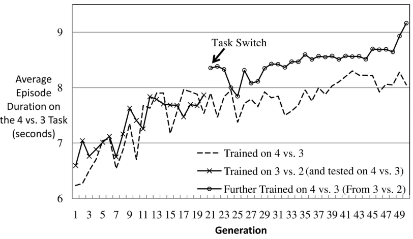
Figure 10: Transfer Learning From 3 vs. 2 to 4 vs. 3 Keepaway on a 25m×25m Field. As the performance (averaged over five runs) of the champion on the 3 vs. 2 task improves, the transfer performance on the 4 vs. 3 task also consequently improves from 6.6 seconds to 8.1 seconds without ever training for it. The improvement is positively correlated (r=0.87).

training for between 50 and 200 hours (depending on the chosen transfer function) beyond the initial bootstrap training in 3 vs. 2 to achieve a comparable 8.0 second episode duration (Taylor et al., 2007b). Thus, because the BEV is static, transfer is instantaneous and requires no special adjustments to the representation to achieve the same result as many hours of further training with the TVITM-PS transfer method.

Although the BEV improves in 4 vs. 3 Keepaway even when only trained in 3 vs. 2, it is still informative to investigate the effect of further training in the 4 vs. 3 task. For this purpose, individ-uals are trained on the 3 vs. 2 task for 20 generations and then further trained on the 4 vs. 3 task for 30 generations. The performance of these policies is contrasted with keepers trained on 4 vs. 3 from scratch for 50 generations. Performance is averaged over five runs and generation champions are evaluated over 1,000 episodes. Figure 11 shows the average test performance of the generation champions. The individuals trained solely on 4 vs. 3 improve from 6.2 seconds to 8.0 seconds. In-terestingly, this performance is equivalent to policies trained only in the 3 vs. 2 task and transferred to 4 vs. 3. However, individuals trained on 3 vs. 2 for the first 20 generations increase their test performance on 4 vs. 3 to 9.1 seconds over the last 30 generations. The final difference between further training after transfer and training from scratch is significant (p<0.05).

Figure 11: Further Training After Transfer From 3 vs. 2 to 4 vs. 3 Keepaway on a 25m×25m Field. Performance of individuals trained on 3 vs. 2 then transferred to 4 vs. 3 and further trained are contrasted with individuals solely trained on 4 vs. 3. All depicted results are performance on the 4 vs. 3 task. Prior training on 3 vs. 2 and transfer to the 4 vs. 3 enhances keeper performance by beginning in a more optimal area of the search space.

it. When training on 4 vs. 3 without previously learning on 3 vs. 2, the third taker’s behavior may inhibit performance by preventing important knowledge from being learned. For example, in 3 vs. 2 an important concept is to pass to the most open player. However, in 4 vs. 3 the most open player is not always the best choice because of the behavior of the third taker; therefore policies that learn the concept of passing to the most open player, which is still an important skill, are not discovered. A thorough evaluation of transfer recognizes that there is more than one way to alter a task. Thus transfer learning is also evaluated by testing the best policy trained in 3 vs. 2 on varied field sizes. Stone et al. (2001) previously investigated this kind of transfer on their best Sarsa solution in an easier version of the Keepaway task that does not include noise by testing a single high-performing individual that was trained on a fixed field size (15m×15m) not only on the trained field size, but also on the other two field sizes. The best policy trained by the HyperNEAT BEV (which, unlike Sarsa, was subject to noise) on the 15m×15m field size was also tested in this way (Figure 12).

Figure 12: 3 vs. 2 Transfer Performance To Larger Field Sizes. Transfer to larger field sizes is eval-uated by testing an individual trained on a single field size (15m×15m) on two larger field sizes (20m×20m and 25m×25m) as well. The BEV is scaled by matching the substrate size to the field size, thus maintaining the same field area represented by each discrete unit on the substrate. Depicted results from Stone and Sutton (2001) show that as a policy trained by Sarsa is transferred to larger field sizes, it decreases in perfor-mance. However, the task is easier as field size increases, as shown by the performance of hand-designed policies (Random, Always Hold, and Hand-Tuned) that increase in performance as field size increases. In contrast, the BEV learns a policy that outper-forms the hand-designed policies and transfers to the larger field sizes, significantly improving performance.

transferred to larger fields. However, even hard-coded policies, such as Random, Always Hold, or Hand Tuned, increase in performance as field size increases, demonstrating the decreased difficulty of the task. Also, in contrast to Sarsa, when transferred to larger fields, the keepers trained with the HyperNEAT BEV improve performance (as would be expected) from 5.6 seconds to 11.0 sec-onds and 13.8 secsec-onds, respectively, and outperform the hand-designed policies (Figure 12). These improvements make sense because the task should become easier when there is more room on the field.

The BEV’s advantage is that the geometric relationships encoded in the CPPN can be extrap-olated as the field size increases, thereby extending the knowledge from the smaller field size to the newer areas of the larger field. For Sarsa, such extrapolation is not possible because as field size increases, the new areas represent previously unseen distances for which Sarsa was not trained. Sarsa has no means to extrapolate geometric knowledge from the distances it has seen because, un-like the CPPN, the knowledge learned is not a function of the domain geometry (i.e., the geometric relationships on a two-dimensional soccer field). Instead, Sarsa learns a function of the examples presented, which do not explicitly describe the geometry of the domain.

Another important lesson from changing the field size is that BEV performance requires a min-imal resolution. When the field size is 15m×15m, the BEV performance appears to underperform compared to Sarsa. In part, this difference is because Sarsa was tested originally without noise (Stone et al., 2001). A later experiment with Sarsa trained on the 15m×15m with noise (Stone et al., 2005) shows that its performance is similar to the BEV. However, another factor is simply that when the field size is 15m×15m, the BEV resolution is also at 15×15, which may be too low to capture the detail necessary to succeed in the task. Confirming this hypothesis, if the BEV is trained at 30×30 resolution on a 15m×15m field, its performance rises significantly, to 7.1 seconds compared to 7.4s for Sarsa when it is trained with noise on 15m×15m (Stone et al., 2005). This re-sult raises the interesting question of whether resolution can be raised above the training resolution without negative impact, as the next experiment addresses.

The final result in Keepaway is that the knowledge learned through the indirect encoding, that is, the CPPN, is not negatively impacted by later increasing resolution from that at which the BEV was trained. The substrate resolution of the champion individuals from five runs from training on three field sizes (15m×15m, 20m×20m, and 25m×25m) are doubled in each dimension and then tested again on the same field size. For example, a 20×20 BEV becomes 40×40, which means that each input represents one quarter as much of the space as before. This BEV quadruples the number of inputs and outputs while increasing the number of connections by a factor of 16 (from 160,000 to 2,560,000 connections). Table 2 shows that no matter the field size, even massively increasing the resolution does not degrade performance and can even lead to a free performance increase.

PERFORMANCE

TRAININGFIELD SIZE TRAINEDRESOLUTION INCREASEDRESOLUTION

15M×15M 4.6S 5.3S

20M×20M 15.4S 15.9S

25M×25M 16.8S 16.9S

Table 2: Average Performance of the Best Individuals at Different Resolutions. The regularities learned by the indirect encoding are not dependent on the particular substrate resolution and may be extrapolated to higher resolutions. Increasing the number of connections in the substrate by a factor of 16 (by doubling the size of each dimension) does not degrade performance; in fact, it even improves it significantly in some cases.

5.3 Knight Joust Transfer Results

Cross-domain transfer is evaluated from the non-Keepaway task of Knight Joust on a 20×20 grid to 3 vs. 2 Keepaway on a 20m×20m field. Evolution is run for 20 generations on the Knight Joust task and then the champions seed the beginning generations of 3 vs. 2 Keepaway. Further training is then performed over ten additional generations of evolution. Performance in Keepaway of the champion players from Knight Joust is on average 0.3 seconds above the performance of initial random individuals. After one generation of evolution, the best individuals from transfer exceed the raw performance by 0.6 seconds. Finally, after ten further generations, the best individuals with transfer hold the ball for 1.1 seconds longer than without transfer (Figure 13).

The differences are significant (p < 0.05). Thus even preliminary learning in a significantly different domain proved beneficial to the BEV. In contrast, previous transfer results from Knight Joust to Keepaway from Taylor and Stone (2007) demonstrated an initial performance advantage, but after training for five simulator hours (which is less than the duration of ten generations) there was no performance difference between learning with transfer and without it.

Overall, the results establish that the BEV is highly effective in transfer in Keepaway. The next section discusses the deeper implications of these results.

6. Discussion and Future Work

Methods that alter representation remain important tools in task transfer for domains in which the representation must change with the task. However, the BEV shows that a carefully chosen repre-sentation with the right encoding can sometimes eliminate the need to change the reprerepre-sentation, even across different domains.

Figure 13: Transfer Results from Knight Joust to Keepaway. Direct transfer and further training performance averaged over 30 runs is shown. The performance of raw champions from Knight Joust on Keepaway outperforms initial random individual by 0.3 seconds. After one generation, this advantage from transfer increases to 0.6 seconds and at 10 genera-tions the advantage is 1.1 seconds. Thus performance on Keepaway, both instantaneous and with further training, benefits from transfer from the Knight Joust domain with sig-nificance p<0.05.

add the intervening interpretation of the input state analogously to how the visual cortex interprets data from the eye. HyperNEAT substrates with hidden layers have been shown to work in the past in domains without transfer (D’Ambrosio and Stanley, 2008; Clune et al., 2009; Gauci and Stanley, 2010). Thus the prospects are good for expanding the scope of static transfer. Nevertheless, of course the human eye represents an ideal, and not all possible domains are amenable to keeping the representation static. Yet for those that are, the investigation in this paper shows that it can provide an advantage.

The role of representation in transfer is relevant to all approaches to learning because transfer is always an option for extending the scope of learning. Thus encoding research, such as in generative and developmental systems (Bentley and Kumar, 1999; Hornby and Pollack, 2002; Lindenmayer, 1968; Stanley, 2007; Bentley and Kumar, 1999; Turing, 1952), and representation research, such as in relational reinforcement learning (Deroski et al., 2001; Morales, 2003; Tadepalli et al., 2004), is important to machine learning in general. Static representations mean that instead of training a new policy, or retraining a previous one, the same policy can be transferred without change. Additionally, the static nature of the representation allows the same policy to train on multiple tasks simultaneously. For example, a soccer player does not practice by playing only soccer games. Players improve through multiple drills and continually practice in-between games to refine skills.

The encoding of the solution also impacts the kinds of policies that are found. For example, in this paper the policy is encoded by a CPPN that is expressed as a function of the task geometry, which enables the solution to exploit regularities in the geometry and extrapolate to previously un-seen areas of the geometry. It should also be possible to simplify the search for a policy that is a function of the geometry in other learning approaches as well. The challenge is that gradient infor-mation (i.e., error) cannot directly pass through the indirection between the ANN and its generating CPPN. A method that solves this problem would open up the power of indirect encoding to all of RL.

6.1 Prospects for Full RoboCup Soccer

An exciting implication of this work is that the power of static transfer and indirect encoding can potentially bootstrap learning the complete game of soccer. After all, the key elements of soccer are present in Keepaway as well. In fact, the results in this paper demonstrate that a static representation can competitively learn to hold the ball in Keepaway and that this skill transfers immediately through the BEV to variations of that task. The static BEV state representation enables the learned policy to transfer to variations of the task in which the number of players is changed (e.g., 3 vs. 2 to 4 vs. 3). Furthermore, indirectly encoding the policy enables the same policy to be applied to variations of the task in which the geometry has been changed (e.g., moving from 20m×20m to 25m×25m field size) HyperNEAT has also been proven effective in a wide variety of tasks (D’Ambrosio and Stanley, 2008; Clune et al., 2009; Stanley et al., 2009; Gauci and Stanley, 2010).

Interestingly, the Keepaway domain was designed as a stepping stone to scaling machine learn-ing methods to the full RoboCup soccer domain (Stone and Sutton, 2001). The same principles that enable the BEV to transfer among variations of the Keepaway domain also can potentially enable the BEV to scale to full Keepaway soccer. For example, because the representation remains static no matter how many players are on the field, training can begin with a small number of players, such as 3 vs. 3 soccer, and iteratively add more players, eventually scaling up to the full 11 vs. 11 soccer game. Furthermore, varying the substrate configuration while the solution encoding remains static makes it possible to train skills relevant to RoboCup on subsets of the full field, for example, half-field offense/defense. In this way, varying the number of players and varying the field size are both required to transfer from the RoboCup Keepaway domain to full RoboCup soccer. Thus this study suggests a novel path to learning full-fledged soccer.

other actions that are possible, such as clearing the ball, kicking the ball out of bounds, dribbling, and passing to a location close to a teammate. Furthermore, the BEV can potentially control players without the ball. By requesting actions in the BEV geometry, actions can be selected based on positions instead of objects.

For example, the keeper with the ball can potentially select any position on the BEV to which to kick the ball. That way, the BEV is not constrained in its actions. The player with the ball can then choose from passes to teammates, passes to positions near teammates, or dribble by kicking the ball to a nearby position and then pursuing the ball. Players without the ball can be controlled by interpreting the outputs of the BEV as the desired location towards which that player should move. Thus an interesting property of the BEV is that the state space can transfer, by accommodating new players or field sizes, and the action space can also transfer in the same way. Ultimately, the promise of such transfer is tied to the idea of static representation, whose potential was highlighted in this paper.

7. Conclusion

This paper introduced the BEV representation, which simplifies task transfer by making the state representation static. That way, no matter how many objects are in the domain, the size of the state representation remains the same. In contrast, in traditional representations, changing the number of players (e.g., in the RoboCup Keepaway task) forces changes in the representation by adding dimensions to the state space. In addition to results competitive with leading methods on the Keep-away benchmark, the BEV, which is enabled by an indirect encoding, achieved transfer learning from 3 vs. 2 to 4 vs. 3 Keepaway without further training. Improvement after further training then demonstrated that the knowledge gained from the transfer does indeed facilitate further learning the more difficult task. Transfer also proved successful not only among variations on the number of players, but also among different field sizes and substrate resolutions. Finally, cross-domain transfer was demonstrated, from Knight Joust to Keepaway. The cross-domain transfer improved not only immediate performance, but also enhanced further learning. All these results highlight the critical role that representation plays in learning and transfer. By altering the representation, transfer learn-ing is simplified. Yet high-dimensional static representations require indirect encodlearn-ings that take advantage of their expressive power, such as in HyperNEAT. The hope is that advanced represen-tations in conjunction with indirect encoding can later contribute to scaling learning techniques to more challenging tasks, such as the complete RoboCup soccer domain.

Acknowledgments

This research is supported in part by a Science, Mathematics, and Research for Transformation (SMART) fellowship from the American Society of Engineering Education (ASEE) and the Naval Postgraduate School.

References

Lee Altenberg. Evolving better representations through selective genome growth. In Proceedings of the IEEE World Congress on Computational Intelligence, pages 182–187, Piscataway, NJ, 1994. IEEE Press.

Peter J. Angeline, Gregory M. Saunders, and Jordan B. Pollack. An evolutionary algorithm that constructs recurrent neural networks. IEEE Transactions on Neural Networks, 5:54–65, 1993.

Petet J. Bentley and Sanjeev Kumar. The ways to grow designs: A comparison of embryogenies for an evolutionary design problem. In Proceedings of the Genetic and Evolutionary Computation Conference (GECCO-1999), pages 35–43, San Francisco, 1999. Kuafmann.

Luigi Cardamone, Daniele Loiacono, and Pier Luca Lanzi. On-line neuroevolution applied to the open racing car simulator. In Proceedings of the 2009 IEEE Congress on Evolutionary Compu-tation (IEEE CEC 2009), Piscataway, NJ, USA, 2009. IEEE Press.

Rich Caruana. Multitask learning. In Machine Learning, pages 41–75, 1997.

Mao Cheny, Klaus Dorer, Ehsan Foroughi, Fredrik Heintz, ZhanXiang Huangy, Spiros Kapetanakis, Kostas Kostiadis, Johan Kummeneje, Jan Murray, Itsuki Noda, Oliver Obst, Pat Riley, Timo Steffens, Yi Wangy, and Xiang Yin. Robocup Soccer Server: User’s Manual. The Robocup Federation, 4.00 edition, February 2003.

Peter Clark. Machine and Human Learning. London: Kogan Page, 1989.

Jeff Clune, Benjamin E. Beckmann, Charles Ofria, and Robert T. Pennock. Evolving coordinated quadruped gaits with the hyperneat generative encoding. In Proceedings of the IEEE Congress on Evolutionary Computation (CEC-2009) Special Section on Evolutionary Robotics, Piscataway, NJ, USA, 2009. IEEE Press.

Ronan Collobert and Jason Weston. A unified architecture for natural language processing: Deep neural networks with multitask learning. In Proceedings of the 25th International Conference on Machine Learning, New York, NY, 2008. ACM Press.

David D’Ambroiso and Kenneth O. Stanley. Evolving policy geometry for scalable multiagent learning. In Proceedings of the Ninth International Conference on Autonomous Agents and Mul-tiagent Systems (AAMAS-2010), page 8, New York, NY, USA, 2010. ACM Press.

David B. D’Ambrosio and Kenneth O. Stanley. Generative encoding for multiagent learning. In Proceedings of the Genetic and Evolutionary Computation Conference (GECCO 2008), New York, NY, 2008. ACM Press.

Carlos Diuk, Andre Cohen, and Michael L. Littman. An object-oriented representation for efficient reinforcement learning. In ICML ’08: Proceedings of the 25th International Conference on Machine learning, pages 240–247, New York, NY, USA, 2008. ACM. ISBN 978-1-60558-205-4. doi: http://doi.acm.org/10.1145/1390156.1390187.