Efficient Learning with Partially Observed Attributes

Efficient Learning with Partially Observed Attributes

∗

Nicol`o Cesa-Bianchi [email protected]

DSI, Universit`a degli Studi di Milano via Comelico, 39

20135 Milano, Italy

Shai Shalev-Shwartz [email protected]

The Hebrew University

Givat Ram, Jerusalem 91904, Israel

Ohad Shamir [email protected]

Microsoft Research One Memorial Drive Cambridge, MA 02142, USA

Editor: Russ Greiner

Abstract

We investigate three variants of budgeted learning, a setting in which the learner is allowed to access a limited number of attributes from training or test examples. In the “local budget” setting, where a constraint is imposed on the number of available attributes per training example, we design and analyze an efficient algorithm for learning linear predictors that actively samples the attributes of each training instance. Our analysis bounds the number of additional examples sufficient to compensate for the lack of full information on the training set. This result is complemented by a general lower bound for the easier “global budget” setting, where it is only the overall number of accessible training attributes that is being constrained. In the third, “prediction on a budget” setting, when the constraint is on the number of available attributes per test example, we show that there are cases in which there exists a linear predictor with zero error but it is statistically impossible to achieve arbitrary accuracy without full information on test examples. Finally, we run simple experiments on a digit recognition problem that reveal that our algorithm has a good performance against both partial information and full information baselines.

Keywords: budgeted learning, statistical learning, linear predictors, learning with partial informa-tion, learning theory

1. Introduction

Consider the problem of predicting whether a person has some disease based on medical tests. In principle, we may draw a sample of the population, perform a large number of medical tests on each person in the sample, and use this information to train a classifier. In many situations, however, this approach is unrealistic. First, patients participating in the experiment are generally not willing to go through a large number of medical tests. Second, each test has some associated cost, and we typically have a budget on the amount of money to spend for collecting the training information. This scenario, where there is a hard constraint on the number of training attributes the

learner has access to, is known asbudgeted learning.1 _{Note that the constraint on the number of}

training attributes may be local (no single participant is willing to undergo many tests) or global (the overall number of tests that can be performed is limited). In a different but related budgeted learning setting, the system may be facing a restriction on the number of attributes that can be viewed at test time. This may happen, for example, in a search engine, where a ranking of web pages must be generated for each incoming user query and there is no time to evaluate a large number of attributes to answer the query.

We may thus distinguish three basic budgeted learning settings:

• Local Budget Constraint: The learner has access to at most k attributes of each individual example, where k is a parameter of the problem. The learner has the freedom to actively choose which of the attributes is revealed, as long as at most k of them will be given.

• Global Budget Constraint: The total number of training attributes the learner is allowed to see is bounded by k. As in the local budget constraint setting, the learner has the freedom to actively choose which of the attributes is revealed. In contrast to the local budget constraint setting, the learner can choose to access more than k/m attributes from specific examples

(where m is the overall number of examples) as long as the global number of attributes is bounded by k.

• Prediction on a budget: The learner receives the entire training set, however, at test time, the predictor can see at most k attributes of each instance and then must form a prediction. The predictor is allowed to actively choose which of the attributes is revealed.

In this paper we focus on budgeted linear regression, and prove negative and positive learning results in the three abovementioned settings. Our first result shows that, under a global budget constraint, no algorithm can learn a general d-dimensional linear predictor while observing less than Ω(d)attributes at training time. This is complemented by the following positive result: we show an efficient algorithm for learning under a givenlocal budget constraint of 2k attributes per example, for any k≥1. The algorithm actively picks which attributes to observe in each example in a randomized way depending on past observed attributes, and constructs a “noisy” version of all attributes. Intuitively, we can still learn despite the error of this estimate because instead of receiving the exact value of each individual example in a small set it suffices to get noisy estimations of many examples. We show that the overall number of attributes our algorithm needs to learn a regressor is at most a factor of d bigger than that used by standard regression algorithms that view all the attributes of each example. Ignoring logarithmic factors, the same gap of d exists when the attribute bound of our algorithm is specialized to the choice of parameters that is used to prove the abovementioned Ω(d)lower bound under the global budget constraint.

In the prediction on a budget setting, we prove that in general it is not possible (even with an infinite amount of training examples) to build an active classifier that uses at most two attributes of each example at test time, and whose error will be smaller than a constant. This in contrast with the local budget setting, where it is possible to learn a consistent predictor by accessing at most two attributes of each example at training time.

2. Related Work

The notion of budgeted learning is typically identified with the “global budget” and “prediction on a budget” settings—see, for example, Deng et al. (2007), Kapoor and Greiner (2005a,b) and Greiner et al. (2002) and references therein. The more restrictive “local budget” setting has been first proposed in Ben-David and Dichterman (1998) under the name of “learning with restricted focus of attention”. Ben-David and Dichterman (1998) considered binary classification and showed learnability of several hypothesis classes in this model, like k-DNF and axis-aligned rectangles. However, to the best of our knowledge, no efficient algorithm for the class of linear predictors has been so far proposed.2

Our algorithm for the local budget setting actively chooses which attributes to observe for each example. Similarly to the heuristics of Deng et al. (2007), we borrow ideas from the adversarial multi-armed bandit problem (Auer et al., 2003; Cesa-Bianchi and Lugosi, 2006). However, our algorithm is guaranteed to be attribute efficient, comes with finite sample generalization bounds, and is provably competitive with algorithms which enjoy full access to the data. A related but different setting is multi-armed bandit on a global budget—see, for example, Guha and Munagala (2007) and Madani et al. (2004). There one learns the single best arm rather than the best linear combination of many attributes, as we do here. Similar protocols were also studied in the context of active learning (Cohn et al., 1994; Balcan et al., 2006; Hanneke, 2007, 2009; Beygelzimer et al., 2009), where the learner can ask for the target associated with specific examples.

Finally, our technique is reminiscent of methods used in the compressed learning framework (Calderbank et al., 2009; Zhou et al., 2009), where data is accessed via a small set of random linear measurements. Unlike compressed learning, where learners are both trained and evaluated in the compressed domain, our techniques are mainly designed for a scenario in which only the access to training data is restricted.

We note that a recent follow-up work (Hazan and Koren, 2011) present 1-norm and 2-norm based algorithms for our local budget setting, whose theoretical guarantees improve on those pre-sented in this paper, and match our lower bound to within logarithmic factors.

3. Linear Regression

We consider linear regression problems where each example is an instance-target pair,(x,y)_∈Rd× R. We refer to x as a vector of attributes. Throughout the paper we assume that _kx_k∞≤1 and

|y_{| ≤}B. The goal of the learner is to find a linear predictor x_{7→ h}w,x_i. In the rest of the paper, we use the term predictor to denote the vector w_∈Rd. The performance of a predictor w on an instance-target pair,(x,y)_∈Rd×R, is measured by a loss functionℓ(_hw,x_i,y). For simplicity, we focus on the squared loss function, ℓ(a,b) = (a₋b)2_{, and briefly mention other loss functions in}

Section 8. Following the standard framework of statistical learning (Haussler, 1992; Devroye et al., 1996; Vapnik, 1998), we model the environment as a joint distribution

D

over the set of instance-target pairs, Rd×R. The goal of the learner is to find a predictor with low risk, defined as the expected loss

LD(w)

def

= E

(x,y)∼D

ℓ(_hw,x_i,y).

Since the distribution

D

_{is unknown, the learner relies on a training set of m examples}

S=(x1,y1), . . . ,(xm,ym) , which are assumed to be sampled i.i.d. from

D

. We denote the training loss by

LS(w)

def = 1

m

m

∑

i=1

(_hw,xii −yi)2.

4. Impossibility Results

Our first result states that any budget learning algorithm (local or global) needs in general a budget ofΩ(d)attributes for learning a d-dimensional linear predictor.

Theorem 1 For any d_≥4 andε_∈ 0,₁₆1, there exists a distribution

D

over_{−1,+1_}d_×{−1,+1_}

and a weight vector w⋆_∈Rd, with_kw⋆_k0=1 andkw⋆k2=kw⋆k1=2√ε, such that any learning algorithm must see at least

k_≥1

2

d

96ε

attributes in order to learn a linear predictor w such that LD(w)−LD(w⋆)<ε.

The proof is given in the Appendix. In Section 6 we prove that under the same assumptions as those of Theorem 1, it is possible to learn a predictor using a local budget of two attributes per example and using a total of

O

e(d2)training examples. Thus, ignoring logarithmic factors hidden in the

O

e notation, we have a multiplicative gap of d between the lower bound and the upper bound.

Next, we consider the prediction on a budget setting. Greiner et al. (2002) studied this setting and showed positive results regarding (agnostic) PAC-learning of k-active predictors. A k-active predictor is restricted to use at most k attributes per test example x, where the choice of the i-th attribute of x may depend on the values of the i₋1 attributes of x that have been already observed. Greiner et al. (2002) show that it is possible to learn a k-active predictor from training examples whose performance is slightly worse than that of the best k-active predictor. But, how good are the predictions of the best k-active predictor? We now show that even in simple cases in which there exists a linear predictor w⋆ with LD(w⋆) =0, the risk of the best k-active predictor can be high.

The following theorem indeed shows that if the only constraint on w⋆is boundedℓ2norm, then the

risk can be as high as 1₋k_d. We use the notation LD(A)to denote the expected loss of the k-active

predictor A on a test example.

Theorem 2 There exists a weight vector w⋆_∈Rd and a distribution

D

such that_kw⋆_k2=1 and LD(w⋆) =0, while any k-active predictor A must have LD(A)≥1−k_d.

Note that the risk of the constant prediction of zero is 1. Therefore, the theorem tells us that no active predictor can get an improvement over the naive predictor of more than _dk.

Proof For any d>k let w⋆= 1√d, . . . ,1√d. Let x_{∈ {±}1_}dbe distributed uniformly at random and y is determined deterministically to be_hw⋆,x_i. Then, LD(w⋆) =0 andkw⋆k2=1. Without loss

all j we therefore obtain

E(yˆ_{− h}w⋆,x_i)2_=E

  yˆ₋

k

∑

i=1

w⋆_ixi− d

∑

j=k+1

w⋆_jxj

!2



=E

  yˆ₋

k

∑

i=1

w⋆_ixi

!2

+

d

∑

j=k+1

(w⋆_j)2E[x2_j]

+2 ˆy

d

∑

j=k+1

w⋆_jE[xj]−2 k

∑

i=1

d

∑

j=k+1

w⋆_iw⋆_jE[xi]E[xj]

=E

  yˆ−

k

∑

i=1

w⋆_ixi

!2

+

∑

i>k

(w⋆_i)2_E[x2

i] +0

≥0+d−k d =1−

k d

which concludes our proof.

It is well known that a low 1-norm of w⋆ encourages sparsity of the learned predictor, which nat-urally helps in designing active predictors. The following theorem shows that even if we restrict

w⋆ to have_kw⋆_k1=1, LD(w⋆) =0, andkw⋆k0>k, we still have that the risk of the best k-active

predictor can be non-vanishing.

Theorem 3 There exists a weight vector w⋆ _∈Rd and a distribution

D

such that _kw⋆_k1 =1, LD(w⋆) =0, andkw⋆k0=ck (for c>1) such that any k-active predictor A must have LD(A)≥

1₋1_cck1.

For example, if in the theorem above we choose c=2, then_kw⋆_k0=2k and LD(A)≥ _4k1. If we

choose instead c=k+1

k , thenkw⋆k0=k+1 and LD(A)≥

1

(k+1)2. Note that ifkw⋆k0≤k there is a

trivial way to predict on a budget of k attributes by always querying the attributes corresponding to the non-zero elements of w⋆.

Proof Let

w⋆= _ck1, . . . ,_ck1

| {z }

ck components

,0, . . . ,0

and, similarly to the proof of Theorem2, let x_{∈ {±}1_}d be distributed uniformly at random and let

y be determined deterministically to be_hw⋆,x_i. Then, LD(w⋆) =0, kw⋆k1=1, andkw⋆k0=ck.

Without loss of generality, suppose the k-active predictor asks for the first k<ck attributes of a

test example and form its prediction to be ˆy. Again similarly to the proof of Theorem2, since the

x1, . . . ,xk, and on ˆy. Therefore,

E(yˆ_{− h}w⋆,x_i)2=E

  yˆ₋

k

∑

i=1

w⋆_ixi

!2

+

∑

i>k

(w⋆_i)2E[x2_i]

≥0+ck−k (ck)2 =c−1

c2_k =

1₋1

c

1

ck

which concludes our proof.

These negative results highlight an interesting phenomenon: in Section 6 we show that one can learn an arbitrarily accurate predictor w with a local budget of k=2. However, here we show that even if we know the optimal w⋆, we might not be able to accurately predict a new partially observed example unless k is very large. Therefore, at least in the worst-case sense, learning on a budget is much easier than predicting on a budget.

5. Local Budget Constraint: A Baseline Algorithm

In this section we describe a straightforward adaptation of Lasso (Tibshirani, 1996) to the local budget setting. This adaptation is based on a direct nonadaptive estimate of the loss function. In Section 6 we describe a more effective approach, which combines a stochastic gradient descent algorithm called Pegasos (Shalev-Shwartz et al., 2007) with the adaptive sampling of attributes to estimate the gradient of the loss at each step.

A popular approach for learning a linear regressor is to minimize the empirical loss on the training set plus a regularization term, which often takes the form of a norm of the predictor w. For example, in ridge regression the regularization term is_kw_k2₂ and in Lasso the regularization term is_kw_k1. Instead of regularization, we can include a constraint of the form kwk1≤B or kwk2≤ B. Modulo an appropriate choice of the parameters, the regularization form is equivalent to the

constraint form. In the constraint form, the predictor is a solution to the following optimization problem

min w_∈Rd

1

|S_|(x

∑

_,y) ∈S

hw,x_{i −}y2

s.t. _kw_kp≤B

(1)

where S=_{(x1,y1), . . . ,(xm,ym)}is a training set of m examples, B is the regularization parameter, and p is 1 for Lasso and 2 for ridge regression.

We start with a standard risk bound for constrained predictors.

Lemma 4 Let

D

be a distribution on pairs(x,y)_∈Rd×Rsuch that_kx_k∞≤1 and_|y_{| ≤}B holds with probability one. Then there exists a constant c>0 such that

max w :kwk1≤B

LS(w)−LD(w) =c B2

r

1

mln d

δ .

Proof We apply the following Rademacher bound (Kakade et al., 2008)

LS(w)−LD(w)

_≤LmaxB

r

2

mln 2d+ℓmax

r

1

2mln

2 δ

that holds with probability at least 1₋δ for all w_∈Rd such that _kw_k1≤B, where Lmax bounds

the Lipschitz constant for the square loss from above, andℓmaxbounds the square loss from above.

The result then follows by observing that(a₋y)2_−(b−y)2_{≤ |a−b||a+b−2y|. Hence, L} max≤

maxa,b,y|a+b−2y|=4B where both a and b are of the formhw,xi, and we used the fact

_hw,x_i≤B

(recall that_kx_k∞≤1) together with the assumption_|y_{| ≤}B. Similarly, under the same assumptions,

ℓmax=maxa,y(a−y)2=4B2.

This immediately leads to the following risk bound for Lasso.

Corollary 5 Ifw is a minimizer of (1) with p_b =1, then there exists a constant c>0 such that, under

the same assumptions as Lemma 4,

LD(wb)≤ min

w :kwk1≤B

LD(w) +c B2

r

1

mln d

δ (2)

holds with probability at least 1₋δover the random draw of the training set S of size m from

D

.

To adapt Lasso to the partial information case, we first rewrite the squared loss as follows:

hw,x_{i −}y2=w⊤xx⊤w₋2y x⊤w+y2

where w,x are column vectors and w⊤,x⊤are their corresponding transpose (i.e., row vectors). Next, we estimate the matrix xx⊤and the vector x using the partial information we have, and then we solve the optimization problem given in (1) with the estimated values of xx⊤and x. To estimate the vector

x we can pick an index i uniformly at random from[d] =_{1, . . . ,d_}and define the estimation to be a vector v such that

vr=

(

d xr if r=i

0 else . (3)

It is easy to verify that v is an unbiased estimate of x, namely,E[v] =x where expectation is with

respect to the choice of the index i. To estimate the matrix xx⊤ we could pick two indices i,j

independently and uniformly at random from[d], and define the estimation to be a matrix with all zeros except d2xixj in the (i,j) entry. However, this yields a non-symmetric matrix which will make our optimization problem with the estimated matrix non-convex. To overcome this obstacle, we symmetrize the matrix by adding its transpose and dividing by 2. This sampling process can be easily generalized to the case where k>1 attributes can be seen. The resulting baseline procedure3 is given in Algorithm 1.

The following theorem shows that similar to Lasso, the Baseline algorithm is competitive with the optimal linear predictor with a bounded 1-norm.

3. We note that an even simpler approach is to arbitrarily assume that the correlation matrix is the identity matrix and then the solution to the loss minimization problem is simply the averaged vector, w=_∑(x,y)∈Sy x. In that case, we

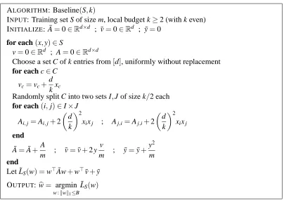
ALGORITHM: Baseline(S,k)

INPUT: Training set S of size m, local budget k_≥2 (with k even) INITIALIZE: ¯A=0_∈Rd×d ; ¯v=0_∈Rd ; ¯y=0

for each(x,y)_∈S

v=0_∈Rd ; A=0_∈Rd×d

Choose a set C of k entries from[d], uniformly without replacement for each c_∈C

vc=vc+

d kxc

Randomly split C into two sets I,J of size k/2 each for each(i,j)_∈I_×J

Ai,j=Ai,j+2

d k

2

xixj ; Aj,i=Aj,i+2

d k

2 xixj end

¯

A=_A¯₊A

m ; ¯v=¯v+2 y v

m ; y¯=y¯+ y2

m

end

Let ˜LS(w) =w⊤Aw¯ +w⊤¯v+y¯ OUTPUT:w_b= argmin

w :_kw_k1≤B

˜LS(w)

Figure 1: An adaptation of Lasso to the local budget setting, where the learner can view at most

k attributes of each training example. The predictive performance of this algorithm is

analyzed in Theorem 6.

Theorem 6 Let

D

be a distribution on pairs(x,y)_∈Rd×Rsuch that_kx_k∞≤1 and_|y_{| ≤}B with probability one. Let ˆw be the output of Baseline(S,k), where_|S_|=m. Then there exists a constant c>0 such that

LD(wˆ)≤ min

w :kwk1≤B

LD(w) +c

d B k

2r

1

mln d

δ

holds with probability of at least 1₋δover the random draw of the training set S from

D

and the algorithm’s own randomization.

The above theorem tells us that for a sufficiently large training set we can find a very good predictor. Put another way, a large number of examples can compensate for the lack of full information on each individual example. In particular, to overcome the extra factor(d/k)2_{in the bound, which does not}

appear in the full information bound given in (2), we need to increase m by a factor of(d/k)4_{. In}

Lemma 7 Let C be a set of n elements and let f : C→Rbe an arbitrary function. Let

C

_k=_{C′⊂ C : _|C′_|=k_}and let U be the uniform distribution over

C

_k. Then

E

C′_∼U

"

1

k_c

∑

′_∈C′

f(c′)

#

= 1

n_c

∑

_∈Cf(c).

Proof We have

E

C′_∼U(

"

1

k_c

∑

′_∈C′

f(c′)

#

= 1_n

k

∑

C′_∈C_k

1

k_c

∑

′_∈C′

f(c′)

= 1

k n_kc

∑

_∈Cf(c)

_{C′∈

C

_{k : c}′_∈C′_}

=

n₋1

k₋1

k n_{k c}

∑

_∈Cf(c)

=1

n_c

∑

_∈Cf(c)

and this concludes the proof.

We now show that the estimation matrix constructed by the Baseline algorithm is likely to be close to the true correlation matrix over the training set.

Lemma 8 Let At be the matrix constructed at iteration t of the Baseline algorithm and note that

¯

A= 1

m∑ m

t=1At. Let X =_m1∑tm=1xtxt⊤. Then, with probability of at least 1−δover the algorithm’s

own randomness we have that

_A¯_{r,s−Xr,s≤}d

k

2s

8

mln

2d2

δ

r,s=1, . . . ,d.

Proof Based on Lemma 7, it is easy to verify thatE[At] =x⊤t xt. Additionally, since we sample without replacements, each element of At is in

h

−2 d_k2,2 d_k2

i

because we assume _kxtk∞≤1. Therefore, we can apply Hoeffding’s inequality on each element of ¯A and obtain that

PhA¯r,s−Xr,s

>εi_≤2 exp ₋mε

2

8

k d

4!

.

Combining the above with the union bound we obtain that

Ph∃(r,s) :A¯r,s−Xr,s

>εi_≤2 d2exp ₋mε

2

8

k d

4!

.

Setting the right-hand side of the above toδand rearranging terms concludes the proof.

Lemma 9 Let vt be the vector constructed at iteration t of the Baseline algorithm and note that

¯v= _m1∑_tm₌₁2 ytvt. Let ¯x= _m1∑tm=12 ytxt. Then, with probability at least 1−δover the algorithm’s

own randomness we have that

k¯v₋¯x_k∞≤dB

k s 8 mln 2d δ .

Proof Based on Lemma 7, it is easy to verify thatE[2 ytvt] =2 ytxt. Additionally, since we sample

k elements without replacement, each element of vt is in

−d k, d k

(because we assume_kxtk∞≤1) and thus each element of 2ytvt is in

−2dB k , 2dB k

(because we assume that_|yt| ≤B). Therefore, we can apply Hoeffding’s inequality on each element of ¯v and obtain that

Phv¯r−x¯r

>εi_≤2 exp ₋mε

2 8 k dB 2! .

Combining the above with the union bound we obtain that

P

h

∃(r,s) :A¯r,s−Xr,s

>εi_≤2d exp −mε 2 8 k dB 2! .

Setting the right-hand side of the above toδand rearranging terms concludes proof.

Next, we show that the estimated training loss

˜LS(w) =w⊤Aw¯ +w⊤¯v+y¯

computed by the Baseline algorithm is close to the true training loss.

Lemma 10 With probability greater than 1₋δover the Baseline algorithm’s own randomization, for all w such that_kw_k1≤B,

˜LS(w)−LS(w)

_≤Bd

k 2s 32 m ln 2d2 δ .

Proof Using twice H¨older’s inequality and Lemma 8 we get

w⊤(A¯₋X)w_{≤ k}w_k1

(A¯₋X)w_{∞≤ k}w_k2₁ max

r,s=1,...,d

(A¯₋X)r,s

≤ Bd k 2s 8 mln 2d2 δ . (4)

Similarly, using H¨older’s inequality and Lemma 9 we also get

Using the triangle inequality, (4)–(5), and the union bound we finally obtain

˜LS(w)−LS(w)

=w⊤Aw¯ +w⊤¯v+y¯₋w⊤X w₋w⊤¯x₋y¯

≤w⊤(A¯₋X)w+w⊤(¯v₋¯x)

≤

Bd k

2s

8

mln

2d2

δ

+B 2_d k

s

8

mln

2d δ

which upon slight simplifications concludes the proof.

We are now ready to prove Theorem 6.

Proof (of Theorem 6) Lemma 4 states that with probability greater than 1₋δover the random draw of a training set S of m examples, for all w such thatkwk1≤B, we have that

LS(w)−LD(w) =c′B2

r

1

mln d

δ

for some c′>0. Combining the above with Lemma 10, we obtain that for some c>0, with proba-bility at least 1₋δover both the random draw of the training set and the algorithm’s own random-ization,

LD(w)−˜LS(w)

_≤LD(w)−LS(w)

+LS(w)−˜LS(w)

_≤c

dB k

2r

1

mln d

δ

for all w such that_kw_k1≤B. The proof of Theorem 6 follows since the Baseline algorithm

mini-mizes ˜LS(w).

6. Gradient-Based Attribute Efficient Regression

In this section, by avoiding the estimation of the matrix xx⊤, we significantly decrease the number of additional examples sufficient for learning with k attributes per training example. To do so, we do not try to estimate the loss function but rather to estimate the gradient∇ℓ(w) =2 _hw,x_{i −}yx, with

respect to w, of the squared loss functionℓ(w) = _hw,x_{i −}y2. Each vector w defines a probability distribution P over [d] by letting P(i) =_|wi|kwk1. We can estimate the gradient using an even

number k_≥2 of attributes as follows. First, we randomly pick a subset i1, . . . ,ik/2from[d]according

to the uniform distribution over the k/2-subsets in[d]. Based on this, we estimate the vector x via

v=2 kd

k/2

∑

s=1

xiseis (6)

where ej is the j-th element of the canonical basis ofRd. Second, we randomly pick j1, . . . ,jk/2

from[d]without replacement according to the distribution defined by w. Based on this, we estimate the term_hw,x_iby

ˆ

y=2 kkwk1

k/2

∑

s=1

sgn wjs

xjsejs . (7)

Lemma 11 Fix any w,x∈Rd and y∈Rand letℓ(w) = _hw,xi −ybe the square loss. Then the estimate

e

∇ℓ(w) =2 ˆy₋yv (8)

satisfiesE∇eℓ(w) =2 _hw,x_{i −}yx=∇ℓ(w).

Proof Since E[d xjej] =x for a random j ∈[d], Lemma 7 immediately implies that E[v] =x. Moreover, it is easy to see that Ekw_k1sgn(wi)xiei

=_hw,x_i when i is drawn with probability

P(i) =_|wi|

kw_k1. HenceE[yˆ] =hw,xi. The proof is concluded by noting that i1, . . . ,ik/2are drawn

independently from j1, . . . ,jk/2.

The advantage of the above approach over the loss based approach we took before is that the mag-nitude of each element of the gradient estimate is order of d_kw_k1. This is in contrast to what we had

for the loss based approach, where the magnitude of each element of the matrix A was order of d2. In many situations, the 1-norm of a good predictor is significantly smaller than d and in these cases the gradient based estimate is better than the loss based estimate. However, while in the previous approach our estimation did not depend on a specific w, now the estimation depends on w. We therefore need an iterative learning method in which at each iteration we use the gradient of the loss function on an individual example. Luckily, the stochastic gradient descent approach conveniently fits our needs.

Concretely, below we describe a variant of the Pegasos algorithm (Shalev-Shwartz et al., 2007) for learning linear regressors. Pegasos tries to minimize the regularized risk

min w

λ 2kwk

2

2 + E

(x,y)∼D h

hw,x_{i −}y2i. (9)

Of course, the distribution

D

is unknown, and therefore we cannot hope to solve the above problem exactly. Instead, Pegasos finds a sequence of weight vectors that (on average) converge to the solution of (9). We start with the all zeros vector w=0_∈Rd_{. Then, at each iteration Pegasos picks} the next example in the training set (which is equivalent to sampling a fresh example according to

D

) and calculates the gradient of the regularized loss

g(w) =λ

2kwk

2

2+ hw,xi −y

2

for this example with respect to the current weight vector w. This gradient is simply ∇g(w) =

λw+∇ℓ(w), where∇ℓ(w) =2 _hw,x_{i −}yx. Finally, Pegasos updates the predictor according to

the gradient descent rule w_←w_−λ1_t∇g(w) where t is the current iteration number. This can be rewritten as w_← 1₋1_tw_−λ1_t∇ℓ(w).

To apply Pegasos in the partial information case we could simply replace the gradient vector ∇ℓ(w)with its estimation given in (8). However, our analysis shows that it is desirable to maintain an estimation vector∇eℓ(w) with small magnitude. Since the magnitude of∇eℓ(w) =2 ˆy−yv is

order of d_kw_k1, we would like to ensure thatkwk1 is always smaller than some threshold B. We

achieve this goal by adding an additional projection step at the end of each Pegasos’s iteration. Formally, the update is performed in two steps as follows

w←

1−1 t

w−_λ1

t2 ˆy−y

v (10)

w_← argmin

u :kuk1≤B

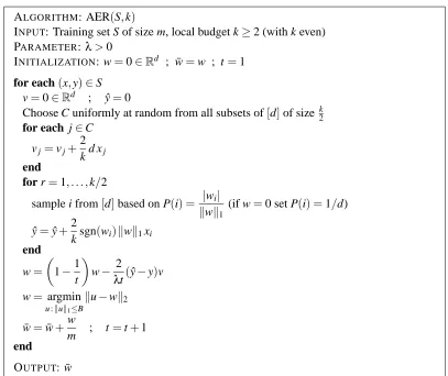
ALGORITHM: AER(S,k)

INPUT: Training set S of size m, local budget k_≥2 (with k even) PARAMETER:λ>0

INITIALIZATION: w=0∈Rd ; ¯w=w ; t=1

for each(x,y)_∈S v=0∈Rd ; yˆ=0

Choose C uniformly at random from all subsets of[d]of size k₂ for each j_∈C

vj=vj+ 2

kd xj

end

for r=1, . . . ,k/2

sample i from[d]based on P(i) = |wi| kw_k1

(if w=0 set P(i) =1/d)

ˆ

y=yˆ+2

ksgn(wi)kwk1xi

end

w=

1₋1

t

w₋ 2

λt(yˆ−y)v

w= argmin

u :kuk1≤B

ku₋w_k2

¯

w=w¯ +w

m ; t=t+1

end

OUTPUT: ¯w

Figure 2: An adaptation of the Pegasos algorithm to the local budget setting. Theorem 12 provides a performance guarantee for this algorithm.

where v and ˆy are respectively defined by (6) and (7). The projection step (11) can be performed

efficiently in time

O

(d)using the technique described in Duchi et al. (2008). A pseudo-code of the resulting Attribute Efficient Regression algorithm is given in Figure 2.

Note that the right-hand side of (10) is w_−λ1_t∇f for the function

f(w) =λ_2kw_k2₂+2(yˆ₋y)_hv,w_i. (12) This observation is used in the proof of the following result, providing convergence guarantees for AER.

Theorem 12 Let

D

be a distribution on pairs(x,y)_∈Rd×Rsuch that_kx_k∞≤1 and_|y_{| ≤}B with probability one. Let S be a training set of size m and let ¯w be the output of AER(S,k) run with

λ=12dplog(m)/(mk). Then, there exists a constant c>0 such that

LD(w¯)≤ min

w :kwk1≤B

LD(w) +c dB2

r

1

kmln m

holds with probability at least 1−δover both the choice of the training set and the algorithm’s own randomization.

Proof Let yt,yˆt,vt,wt be the values of y,yˆ,v,w, respectively, at each iteration t of the AER algorithm. Moreover, let∇t=2(_hwt,xti −yt)xt and∇te =2(yˆt−yt)vt. From the convexity of the squared loss, and taking expectation with respect to the algorithm’s own randomization, we have that for any vector w⋆such that_kw⋆_k1≤B,

E

"

m

∑

t=1

hwt,xti −yt

2

#

−

m

∑

t=1

hw⋆,xti −yt

2 ≤E

"

m

∑

t=1

h∇t,wt−w⋆i

#

=E

"

m

∑

t=1

h∇te ,wt−w⋆i

#

=E

"

m

∑

t=1

2(yˆt−yt)hvt,wt−w⋆i

#

.

For the first equality we used Lemma 11, which states that, conditioned on wt,Ee∇t

=∇t. We now deterministically bound the random quantity inside the above expectation as follows

m

∑

t=1

2(yˆt−yt)hvt,wt−w⋆i= m

∑

t=1

_λ

2kwtk

2

2+2(yˆt−yt)hvt,wti

−

m

∑

t=1

_λ

2kw

⋆

k22+2(yˆt−yt)hvt,w⋆i

+mλ

2kw

⋆ k22

=

m

∑

t=1

ft(wt)− m

∑

t=1

ft(w⋆) +m λ 2kw

⋆ k22

where ft(w) =λ₂kwk22+2(yˆt−yt)hvt,wiis theλ-strongly convex function defined in (12). Recalling that the right-hand side in the AER update (10) is equal to wt− 1

λt∇ft(wt), we can apply the fol-lowing logarithmic regret bound forλ-strongly convex functions (Hazan et al., 2006; Kakade and Shalev-Shwartz, 2008)

m

∑

t=1

ft(wt)− m

∑

t=1

ft(w⋆)≤ 1 λ

max

t k∇ft(wt)k

2_{ln m}

which remains valid also in the presence of the projection steps (11). Similarly to the analysis of Pegasos, and using our assumptions on_kxtk∞and|yt|, the norm of the gradient∇ft(wt)is bounded as follows

∇ft(wt)

_≤λkwtk+2

yˆt−yt

_kvtk ≤λkwtk+4Bd

r

2

k .

In addition, it is easy to verify (e.g., using an iductive argument) that

kwtk ≤ 1 λ4Bd r 2 k, which yields

∇ft(wt)

_≤8Bd

r

2

This gives the bound

m

∑

t=1

2(yˆt−yt)hvt,wt−w⋆i ≤

128(dB)2

λk ln m+m

λ 2kw

⋆_k2

2.

Choosingλ=16dplog(m)/(km)and noting thatk · k2≤ k · k1we get that

m

∑

t=1

2(yˆt−yt)hvt,wt−w⋆i ≤16dB2

r

m k ln m.

The resulting bound is then

E

"_m

∑

t=1

hwt,xti −yt

2

#

≤

m

∑

t=1

hw⋆,xti −yt

2

+16dB2

r

m k ln m.

To conclude the proof, we apply the online-to-batch conversion of Cesa-Bianchi et al. (2004, Corol-lary 2) to the probability space that includes both the algorithm’s own randomization and the prod-uct distribution from which the training set is drawn. Since _hw,xti −yt

2

≤4B2 for all w such that_kw_k1≤B (recall our assumptions on xt and yt), and using the convexity of the square loss, we obtain that

LD(w¯)≤ inf

w :kwk≤BLD(w) +16dB

2

r

1

kmln m+4B 2

r

2

mln

1 δ holds with probability at least 1₋δwith respect to all random events.

Note that for small values of k (which is the reasonable regime here) the bound for AER is much better than the bound for Baseline: ignoring logarithmic factors, instead of quadratic dependence on d, we have only linear dependence on d.

It is interesting to compare the bound for AER to the Lasso bound (2) for the full information case. As it can be seen, to achieve the same level of risk, AER needs a factor of d2/k more examples

than the full information Lasso.4 Since each AER example uses only k attributes while each Lasso example uses all d attributes, the ratio between the total number of attributes AER needs and the number of attributes Lasso needs to achieve the same error is

O

(d). Intuitively, when having d times total number of attributes, we can fully compensate for the partial information protocol.

However, in some situations even this extra d factor is not needed. Indeed, suppose we know that the vector w⋆, which minimizes the risk, is dense. That is, it satisfieskw⋆k1≈

√

dkw⋆k2≤B.

In this case, by settingλ=d3/2plog(m)/(km), and using the tighter bound_kw⋆_k2≤B √

d instead

of_kw⋆_k2≤ kw⋆k1≤B in the proof of Theorem 12, we get a final bound of the form LD(w¯)≤LD(w⋆) +c B2

r

d kmln

m

δ .

Therefore, the number of examples AER needs in order to achieve the same error as Lasso is only a factor d/k more than the number of examples Lasso uses. But, this implies that both AER and

Lasso needs the same number of attributes in order to achieve the same level of error! Crucially, the above holds only if w⋆ is dense. When w⋆ is sparse we have_kw⋆_k1≈ kw⋆k2 and then AER needs

more attributes than Lasso.

4. We note that when d=k we still do not recover the full information bound. However, it is possible to improve the

analysis and replace the factor d/√k with a factor d maxtkxtk2

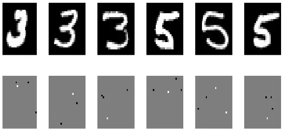
Figure 3: In the upper row six examples from the training set (of digits 3 and 5) are shown. In the lower row we show the same six examples, where only four randomly sampled pixels from each original image are displayed.

7. Experiments

We performed some experiments to test the behavior of our algorithm on the well-known MNIST digit recognition data set (Le Cun et al., 1998), which contains 70,000 images (28_×28 pixels each) of the digits 0₋9. The advantages of this data set for our purposes is that it is not a small scale data set, has a reasonable dimensionality-to-data-size ratio, and the setting is clearly interpretable graphically. While this data set is designed for classification (e.g., recognizing the digit in the image), we can still apply our algorithms on it by regressing to the label.

First, to demonstrate the hardness of our settings, we provide in Figure 3 below some examples of images from the data set, in the full information setting and the partial information setting. The upper row contains six images from the data set, as available to a full information algorithm. A partial information algorithm, however, will have a much more limited access to these images. In particular, if the algorithm may only choose k=4 pixels from each image, the same six images as available to it might look like the bottom row of Figure 3.

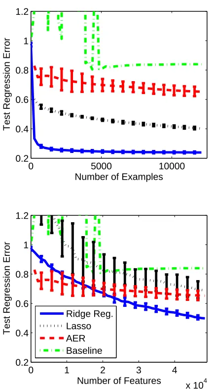
We began by looking at a data set composed of “3” vs. “5”, where all the “3” digits were labeled as₋1 and all the “5” digits were labeled as+1. We ran four different algorithms on this data set: the simple Baseline algorithm, AER, as well as ridge regression and Lasso for comparison (for Lasso, we solved (1) with p=1). Both ridge regression and Lasso were run in the full information setting: Namely, they enjoyed full access to all attributes of all examples in the training set. The Baseline algorithm and AER, however, were given access to only four attributes from each training example. We randomly split the data set into a training set and a test set (with the test set being 10% of the original data set). For each algorithm, parameter tuning was performed using 10-fold cross valida-tion. Then, we ran the algorithm on increasingly long prefixes of the training set, and measured the average regression error(_hw,x_{i −}y)2_{on the test set. The results (averaged over runs on 10 random}

The bottom plot of Figure 4 is similar, only that now the X -axis represents the accumulative number of attributes seen by each algorithm rather than the number of examples. For the partial-information algorithm, the graph ends at approximately 49,000 attributes, which is the total number of attributes accessed by the algorithm after running over all training examples, seeing k=4 pixels from each example. However, for the full-information algorithms 49,000 attributes are already seen after just 62 examples. When we compare the algorithms in this way, we see that our AER algorithm achieves excellent performance for a given attribute budget, significantly better than the other 1-norm-based algorithms (Baseline and Lasso). Moreover, AER is even comparable to the full information 2-norm-based ridge regression algorithm, which performs best on this data set.

0 5000 10000

0.2 0.4 0.6 0.8 1 1.2

Number of Examples

Test Regression Error

0 1 2 3 4

x 104

0.2 0.4 0.6 0.8 1 1.2

Number of Features

Test Regression Error

Ridge Reg. Lasso AER Baseline

Finally, we tested the algorithms over 45 data sets generated from MNIST, one for each possible pair of digits. For each data set and each of 10 random train-test splits, we performed parameter tuning for each algorithm separately, and checked the average squared error on the test set. The median test errors over all data sets are presented in the table below.

Test Error

Full Information Ridge 0.110

Lasso 0.222

Partial Information AER 0.320

Baseline 0.812

As can be seen, the AER algorithm manages to achieve good performance, not much worse than the full information Lasso algorithm. The Baseline algorithm, however, achieves a substan-tially worse performance, in line with our theoretical analysis above. We also calculated the test classification error of AER, that is, sign(_hw,x_i)₆=y, and found out that AER, which can see only

4 pixels per image, usually performs only a little worse than the full information algorithms (ridge regression and Lasso), which enjoy full access to all 784 pixels in each image. In particular, the median test classification errors of AER, Lasso, and Ridge are 3.5%, 1.1%,and 1.3% respectively.

8. Discussion and Extensions

In this paper we have investigated three budgeted learning settings with different constraints on the way instance attributes may be accessed: a local constraint on each training example (local budget), a global constraint on the set of all training examples (global budget), and a constraint on each test example (prediction on a budget). In the local budget setting, we have introduced a simple and efficient algorithm, AER, that learns by accessing a pre-specified number of attributes from each training example. The AER algorithm comes with formal guarantees, is provably competitive with algorithms which enjoy full access to the data, and performs well in simple experiments. This result is complemented by a general lower bound for the global budget setting which is a factor d smaller than the upper bound achieved by our algorithm. We note that this gap has been recently closed by Hazan and Koren (2011), which in our local budget setting, show 1-norm and 2-norm-based algorithms for learning linear predictors using only

O

e(d)attributes, thus matching our lower bound to within logarithmic factors.

Whereas AER is based on Pegasos, our adaptive sampling approach easily extends to other gradient-based algorithms. For example, generalized additive algorithms such as p-norm Percep-trons and Winnow—see, for example, Cesa-Bianchi and Lugosi (2006).

In contrast to the local/global budget settings, where we can learn efficiently by accessing few attributes of each training example, we showed that accessing a limited number of attributes at test time is a significantly harder setting. Indeed, we proved that is not possible to build an active linear predictor that uses two attributes of each test example and whose error is smaller than a certain constant, even when there exists a linear predictor achieving zero error on the same data source.

2008), where the goal is to exploit the attribute efficiency property in order to prevent acquisition of information about individual data instances.

Acknowledgments

We would like to thank the anonymous reviewers for their detailed and helpful comments. N. Cesa-Bianchi gratefully acknowledges partial support by the PASCAL2 Network of Excellence under EC grant no. 216886. This publication only reflects the authors’ views.

Appendix A. Proof of Theorem 1

The outline of the proof is as follows. We define a specific distribution such that only one “good” feature is slightly correlated with the label. We then show that if some algorithm learns a linear predictor with an extra risk of at mostε, then it must know the value of the good feature. Next, we construct a variant of a multi-armed bandit problem out of our distribution and show that a good learner can yield a good prediction strategy. Finally, we adapt a lower bound for the multi-armed bandit problem given in Auer et al. (2003), to conclude that the number k of attributes viewed by a good learner must satisfy k=Ω d_ε.

A.1 The Distribution

We generate a joint distribution overRd×Ras follows. Choose some j_∈[d]. First, we generate

y1,y2, . . ._{∈ {±}1_} i.i.d. according toPyt =1=Pyt =−1= 1₂. Given j and yt, xt ∈ {±1} is generated according toPxt,i=yt

= 1

2+1{i= j}p where p>0 is chosen later. Denote by Pj

the distribution mentioned above assuming the “good” feature is j. Also denote byPuthe uniform distribution over_{±1_}d+1. Analogously, we denote byEjandEuexpectations w.r.t.PjandPu. A.2 A Good Regressor “Knows” j

We now show that if we have a good linear regressor than we can know the value of j. It is easy to see that the optimal linear predictor under the distributionPjis w⋆=2p ej, and the risk of w⋆is

L_Pj(w

⋆_{) =E}

j

(_hw⋆,x_{i −}y)2= 1 2+p

(1₋2p)2+ 1 2−p

(1+2p)2=1+4p2₋8p2=1₋4p2. The risk of an arbitrary weight vector w under Pjis

LPj(w) =Ej

(_hw,x_{i −}y)2=

∑

i6=j

w2_i +Ej

(wjxj−y)2

=

∑

i6=j

w2_i +w2_j+1₋4pwj.

Suppose that LPj(w)−LPj(w

⋆_{)<ε. This implies that:}

1. For all i₆= j we have w2_i <ε, or equivalently,_|wi|<√ε.

2. 1+w2_j−4pwj−(1−4p2)<εand thus|wj−2p|<√εwhich gives|wj|>2p−√ε. By choosing p=√ε, the above implies that we can identify the value of j from any w whose risk

is strictly smaller than L_Pj(w

A.3 Constructing A Variant Of A Multi-Armed Bandit Problem

We now construct a variant of the multi-armed bandit problem out of the distribution Pj. Each coordinate i∈ {1, . . . ,d}is an arm and the reward of pulling i at time t is1{xNi,t,i=yNi,t} ∈ {0,1},

where Ni,t denotes the random number of times arm i has been pulled in the first t plays. Hence the expected reward of pulling i is 1₂+1{i=j_}p. At the end of each round t the player observes xNi,t,i

and yNi,t.

A.4 A Good Learner Yields A Bandit Strategy

Suppose that we have a learner that, for any j=1, . . . ,d, can learn a linear predictor with LPj(w)− LPj(w

⋆_{)<εusing k attributes. Since we have shown that once L}

Pj(w)−LPj(w

⋆_{)<εwe know the}

value of j, we can construct a strategy for the multi-armed bandit problem in a straightforward way. Simply use the first m examples to learn w and from then on always pull the arm j. The expected reward of this strategy under anyPjafter T ≥k plays is at least

k

2+ (T−k)

1 2+p

=T

2 + (T−k)p. (13)

A.5 An Upper Bound On the Reward Of Any Bandit Strategy

Recall that under distributionPj the expected reward for pulling arm I is 1₂+p1{I= j}. Hence, the total expected reward of a player that runs for T rounds is upper bounded by 1₂T+pEj[Nj], where Nj=Nj,T is the overall number of pulls of arm j. Moreover, at the end of each round t the player observes xs,iand ys, where s=Ni,t. This allows the player to compute the value of the reward for the current play. For any s, note that ysis observed whenever some arm i is pulled for the s-th time. However, sincePj

xi,s=ys

=Pj

xi,s=ys|ys

for all i (including i= j), the knowledge of ysdoes not provide any information about the distribution of rewards for arm i. Therefore, without loss of generality, we can assume that at each play the bandit strategy observes only the obtained binary reward. This implies that our bandit construction is identical to the one used in the proof of Theorem 5.1 in Auer et al. (2003). In particular, for any bandit strategy there exists some arm j such that the expected reward of the strategy under distributionPjis at most

T

2 +p

T d +T

r

−T

d ln(1−4p 2₎

!

≤T

2 +p

T d +T

r

6T

d p 2

!

(14)

where we used the inequality₋ln(1₋q)_≤ 3

2q for q∈[0,1/4]. Note that q=4p

2_{=4ε∈[0,1/4]}

whenε_≤1/16.

A.6 Concluding The Proof

Take a learning algorithm that finds anε-good predictor using k attributes. Since the reward of the strategy based on this learning algorithm cannot exceed the upper bound given in (14), from (13) we obtain that

T

2 + (T−k)p≤

T

2 +p

T d +T

r

6T

d p 2

which solved for k gives

k_≥T 1₋1

d−

r

6T

d p 2

!

.

Since we assume d≥4, choosing T=d(96p2), and recalling p2=ε, gives k_≥T

2 =

1 2

d

96ε

.

References

P. Auer, N. Cesa-Bianchi, Y. Freund, and R.E. Schapire. The nonstochastic multiarmed bandit problem. SIAM Journal on Computing, 32, 2003.

M-F Balcan, A. Beygelzimer, and J. Langford. Agnostic active learning. In ICML, 2006.

S. Ben-David and E. Dichterman. Learning with restricted focus of attention. JCSS: Journal of

Computer and System Sciences, 56, 1998.

A. Beygelzimer, S. Dasgupta, and J. Langford. Importance weighted active learning. In ICML, 2009.

R. Calderbank, S. Jafarpour, and R. Schapire. Compressed learning: Universal sparse dimensional-ity reduction and learning in the measurement domain. Manuscript, 2009.

N. Cesa-Bianchi and G. Lugosi. Prediction, Learning, and Games. Cambridge University Press, 2006.

N. Cesa-Bianchi, A. Conconi, and C. Gentile. On the generalization ability of on-line learning algorithms. IEEE Transactions on Information Theory, 50(9):2050–2057, September 2004.

N. Cesa-Bianchi, S. Shalev-Shwartz, and O. Shamir. Online learning of noisy data with kernels. In

COLT, 2010.

D. Cohn, L. Atlas, and R. Ladner. Improving generalization with active learning. Machine Learning, 15:201–221, 1994.

K. Deng, C. Bourke, S. Scott, J. Sunderman, and Y. Zheng. Bandit-based algorithms for budgeted learning. In ICDM, 2007.

L. Devroye, L. Gy¨orfi, and G. Lugosi. A Probabilistic Theory of Pattern Recognition. Springer, 1996.

J. Duchi, S. Shalev-Shwartz, Y. Singer, and T. Chandra. Efficient projections onto theℓ1-ball for

learning in high dimensions. In ICML, 2008.

C. Dwork. Differential privacy: A survey of results. In M. Agrawal, D.-Z. Du, Z. Duan, and A. Li, editors, TAMC, volume 4978 of Lecture Notes in Computer Science, pages 1–19. Springer, 2008.

R. Greiner, A. J. Grove, and D. Roth. Learning cost-sensitive active classifiers. Artificial

S. Guha and K. Munagala. Approximation algorithms for budgeted learning problems. In STOC, 2007.

S. Hanneke. A bound on the label complexity of agnostic active learning. In ICML, 2007.

S. Hanneke. Adaptive rates of convergence in active learning. In COLT, 2009.

D. Haussler. Decision theoretic generalizations of the PAC model for neural net and other learning applications. Information and Computation, 100(1):78–150, 1992.

E. Hazan and T. Koren. Optimal algorithms for ridge and Lasso regression with partially observed attributes. CoRR, abs/1108.4559, 2011.

E. Hazan, A. Kalai, S. Kale, and A. Agarwal. Logarithmic regret algorithms for online convex optimization. In COLT, 2006.

S.M. Kakade and S. Shalev-Shwartz. Mind the duality gap: Logarithmic regret algorithms for online optimization. In Advances in Neural Information Processing Systems 22, 2008.

S.M. Kakade, K. Sridharan, and A. Tewari. On the complexity of linear prediction: Risk bounds, margin bounds, and regularization. In NIPS, 2008.

A. Kapoor and R. Greiner. Learning and classifying under hard budgets. In ECML, 2005a.

A. Kapoor and R. Greiner. Budgeted learning of bounded active classifiers. In Proceedings of the

ACM SIGKDD Workshop on Utility-Based Data Mining, 2005b.

Y. L. Le Cun, L. Bottou, Y. Bengio, and P. Haffner. Gradient-based learning applied to document recognition. Proceedings of IEEE, 86(11):2278–2324, November 1998.

O. Madani, D.J. Lizotte, and R. Greiner. Active model selection. In UAI, 2004.

S. Shalev-Shwartz, Y. Singer, and N. Srebro. Pegasos: Primal Estimated sub-GrAdient SOlver for SVM. In ICML, 2007.

R. Tibshirani. Regression shrinkage and selection via the lasso. J. Royal. Statist. Soc B., 58(1): 267–288, 1996.

V. N. Vapnik. Statistical Learning Theory. Wiley, 1998.

S. Zhou, J. Lafferty, and L. Wasserman. Compressed and privacy-sensitive sparse regression. IEEE