Detection and Classification of Heart Premature Contractions via α-Level Binary Neyman-Pearson Radius Test: A Comparative Study

Detection and Classification of Heart Premature Contractions

via

α

-Level Binary Neyman-Pearson Radius Test: A

Comparative Study

M. R. Homaeinezhad

*

, A. Ghaffari

**

, M. Akraminia

*

, M. Atarod

***

and M. M. Daevaeiha

*

Abstract: The aim of this study is to introduce a new methodology for isolation of ectopic

rhythms of ambulatory electrocardiogram (ECG) holter data via appropriate statistical analyses imposing reasonable computational burden. First, the events of the ECG signal are detected and delineated using a robust wavelet-based algorithm. Then, using Binary Neyman-Pearson Radius test, an appropriate classifier is designed to categorize ventricular complexes into "Normal + Premature Atrial Contraction (PAC)" and "Premature Ventricular Contraction (PVC)" beats. Afterwards, an innovative measure is defined based on wavelet transform of the delineated P-wave namely as P-Wave Strength Factor (PSF) used for the evaluation of the P-wave power. Finally, ventricular contractions pursuing weak P-waves are categorized as PAC complexes; however, those ensuing strong P-waves are specified as normal complexes. The discriminant quality of the PSF-based feature space was evaluated by a modified learning vector quantization (MLVQ) classifier trained with the original QRS complexes and corresponding Discrete Wavelet Transform (DWT) dyadic scale. Also, performance of the proposed Neyman-Pearson Classifier (NPC) is compared with the MLVQ and Support Vector Machine (SVM) classifiers using a common feature space. The processing speed of the proposed algorithm is more than 176,000 samples/sec showing desirable heart arrhythmia classification performance. The performance of the proposed two-lead NPC algorithm is compared with MLVQ and SVM classifiers and the obtained results indicate the validity of the proposed method. To justify the newly defined feature space (σi1, σi2, PSFi), a NPC with the proposed feature space and a MLVQ

classification algorithm trained with the original complex and its corresponding DWT as well as RR interval are considered and their performances were compared with each other. An accuracy difference about 0.15% indicates acceptable discriminant quality of the properly selected feature elements. The proposed algorithm was applied to holter data of the DAY general hospital (more than 1,500,000 beats) and the average values of Se = 99.73% and P+ = 99.58% were achieved for sensitivity and positive predictivity, respectively.

Keywords: ECG Delineation, Discrete Wavelet Transform, Premature Atrial Contraction,

Premature Ventricular Contraction, Modified Learning Vector Quantization, Support Vector Machine, Neyman-Pearson Hypothesis Test.

1

Iranian Journal of Electrical & Electronic Engineering, 2010. Paper first received 4 May 2009 and in revised form 20 July 2010. * The Authors are with Research Engineers of the CardioVascular Research Group (CVRG), Department of Mechanical Engineering, K. Nassir Toosi University of Technology.

Emails: {mrezahomaei, mehdi_akraminia,m_davaeiha}@yahoo.com. ** The Author is with Department of Mechanical Engineering, K. Nassir Toosi University of Technology.

E-mail: [email protected].

*** The Author is with School of Biomedical Engineering, University of Calgary, Alberta, Canada.

E-mail: [email protected]

1 Introduction

Heart is a special myogenic muscle which its constitutive cells (myocytes) possess two important characteristics namely as nervous (electrical) excitability and mechanical tension with force feedback. The heart's rhythm of contraction is controlled by the sino-atrial node (SA node) called the heart pacemaker. This node is a part of the heart’s intrinsic conduction system, made up of specialized myocardial (nodal) cells. Each beat of the heart is set in motion by an electrical signal from the SA node located in the heart’s right atrium. The automatic nature of the heartbeat is

referred to as automaticity which is due to the spontaneous electrical activity of the SA node. The superposition of all myocytes electrical activity on the skin surface causes a detectable potential difference which its detection and registration together is called electrocardiography. However, heart’s electrical system controls all events occurring when heart pumps blood. If, according to any happening, the electro-mechanical function of a region of myocytes encounters a failure, the corresponding abnormal effects will appear in the ECG which is an important part of the preliminary evaluation of a patient suspected to have a heart-related problem. On the other hand, statistical analysis of the ECG parameters in long-term conditions can yield acceptable solutions for the diagnosis of some certain phenomena such as T-Wave Alternans (TWA) [1], Atrial Fibrillation (AF) [2], QT-prolongation [3] and also in applications including pattern recognition and arrhythmia classification [4] in which more accurate results would be achieved with proper delineation of ECG waveforms. Therefore, parameterization and detection of the ECG signal events using a reliable algorithm is the first stage in the computer analysis of the ECG signal. Numerous approaches have yet been developed for the aim of detection of the ECG events including mathematical models [5], Hilbert transform and the first derivative [6-8], second order derivative [9], wavelet transform and the filter banks [10], soft computing (Neuro-fuzzy, genetic algorithm) [11], Hidden Markov Models (HMM) application [12], etc. Several features and extraction (selection) methods have been created and implemented by authors; for instance, original ECG signal [13], preprocessed ECG signal via appropriately defined and implemented transformations such as discrete wavelet transform, continuous wavelet transform [14], Hilbert transform [15], fast Fourier transform [16-17], short time Fourier transform [18], power spectral density [19-20], higher order spectral methods [21-22], statistical moments [23], nonlinear transformations such as Liapunov exponents and fractals [24-26] have been used as appropriate sources for feature extraction. In order to extract feature(s) from a selected source, various methodologies and techniques have been introduced.

After generation of the feature source, segmentation, feature selection and extraction (calculation), the resulted feature vectors should be divided into two groups “train” and “test” to tune an appropriate classifier such as a neural network, support vector machine or ANFIS, [27-37]. Using RR-tachogram or heart rate variability, analysis in feature extraction and via simple if-then or other parametric or nonparametric classification rules [38-40], artificial neural networks, fuzzy or ANFIS networks [41-44], support vector machines [45] and probabilistic frameworks such as Bayesian hypotheses tests [46], the arrhythmia classification would be fulfilled with acceptable accuracies. Heretofore, the main concentration of the

arrhythmia classification schemes has been on morphology assessment and/or geometrical parameters of the ECG events. Traditionally, in the studies based on the morphology and the wave geometry, first, during a preprocessing stage, some corrections such as baseline wander removal, noise-artifact rejection and a suitable scaling are applied. Then, using an appropriate mapping for instance, filter banks, discrete or continuous wavelet transform in different spatial resolutions and etc., more information is derived from the original signal for further processing and analyses. In some researches, original and/or preprocessed signal are used as appropriate features and using artificial neural network or fuzzy classifiers [47-52], parametric and probabilistic classifiers [53-55], the discrimination goals are followed. Although, in such classification approaches, acceptable results may be achieved, however, due to the implementation of the original samples as components of the feature vector, computational cost and burden especially in high sampling frequencies will be very high and the algorithm may take a long time to be trained for a given database. In some other researches, geometrical parameters of QRS complexes such as maximum value to minimum value ratio, area under the segment, maximum slope, summation (absolute value) of point to point difference, ST-segment, PR and QT intervals, statistical parameters such as correlation coefficient of a assumed segment with a template waveform, first and second moments of original or preprocessed signal and etc. are used as effective features [27-32]. The main definition origin of these features is based on practical observations and a priori heuristic knowledge whilst conducted researches have shown that by using these features, convincing results may be reached. On the other hand, some of studies in the literature focus on the ways of choosing and calculating efficient features to create skillfully an efficient classification strategy [33-36]. In the area of nonlinear systems theory, some ECG arrhythmia classification methods on the basis of fractal theory [56], state-space, trajectory space, phase space, Liapunov exponents [57] and nonlinear models [26] have been innovated by researchers. Amongst other classification schemes, structures based on higher order statistics in which to analyze features, a two or more dimensional frequency space is constructed can be mentioned [46, 47]. According to the concept that upon appearance of changes in the morphology of ECG signal caused by arrhythmia, corresponding changes are seen in the frequency domain, therefore, some arrhythmia classifiers have been designed based on the appropriate features obtained from signal fast Fourier transform (FFT), short-time Fourier transform (STFT), auto regressive (AR) models and power spectral density (PSD), [58-59]. Finally, using some polynomials such as Hermite function which has specific characteristics, effective features have been extracted to classify some arrhythmias [60-61]. In this study, first, using an

appropriate ECG events detection-delineation algorithm [62-63], ventricular depolarization (normal, PAC, multi-focal PVCs or combination of them) are detected and segmented. Then, using Binary Neyman-Pearson Radius test, an appropriate classifier is designed to categorize ventricular complexes into "Normal + Premature Atrial Contraction (PAC)" and Premature Ventricular Contraction, "PVC" beats. Afterwards, an appropriate measure is defined based on wavelet transform of the delineated P-wave namely as P-Wave Strength Factor which is used for the evaluation of the P-wave power. Accordingly, P-waves are classified into "weak" and "strong" waves. Finally, ventricular contractions pursuing weak power P-waves are categorized as PAC complexes; however, those with preceding strong power P-waves are specified as normal complexes. The proposed algorithm was applied to holter data of DAY general hospital (more than 1,500,000 beats) and the average values of Se = 99.73% and P+ = 99.58% were achieved for sensitivity and positive prediction, respectively. The performance of the proposed two-lead NPC algorithm is compared with MLVQ and SVM classifiers and the obtained results indicate the validity of the proposed method. On the other hand, to justify the newly defined feature space (σi1, σi2, PSFi), a NPC

with the proposed feature space and a MLVQ classification algorithm trained with the original complex and its corresponding DWT as well as RR interval are considered and their performances were compared with each other. An accuracy difference about 0.04% indicates satisfactory discriminant quality of the properly selected feature elements.

List of abbreviations are as follows:

NPC: Neyman-Pearson Classifier. MLVQ: Modified Learning Vector Quantization. SVM: Support Vector Machine. FAP: False Alarm Probability. pdf: Probability Density Function. LR: Likelihood Ratio. PSF: P-wave Strength Factor. CPUT: CPU Time. ACLM: Area Curve Length Method. ECG: Electrocardiogram. DWT: Discrete Wavelet Transform. SNR: Signal to Noise Ratio. FP: False Positive. FN: False Negative. PVC: Premature Ventricular Contraction. PAC: Premature Atrial Contraction. RCA: Retrograde Conduction into Atrium. FCP: Full Compensatory Pause. TP: True Positive. P+: Positive Predictivity (%). Se: Sensitivity (%). SMF: Smoothing Function. FIR: Finite-duration Impulse Response. CHECK#0: Pocedure of evaluating obtained results using MIT-BIH annotation files.

CHECK#1: Procedure of evaluating obtained results consulted with a control cardiologist.

CHECK#2: Procedure of evaluating obtained results consulted with a control cardiologist and also at least with 3 residents.

2 Materials and Methods

2.1 Discrete Wavelet Transform using à Trous Method

Generally, it can be stated that the wavelet transform is a quasi-convolution of the hypothetical signal x(t) and the wavelet function ψ(t) with the dilation parameter a and translation parameter b, as follows

(

( )

)

, 0 )

( 1 )

( =

∫

+∞ − >

∞

− xt t b a dt a

a b

W_ax ψ (1)

The parameter a can be used to adjust the wideness of the basis function and therefore the transform can be adjusted in temporal resolutions. Suppose that the function Y_ax(b) is obtained based on a quasi-convolution of signal x(t) and function θ(t), as follows

(

t b a

)

dt t

x b

Y_ax

∫

∞ +

∞

− −

= () ( )

)

( θ (2)

If the derivative of Y_ax(b) is calculated relative to b, then

(

t b a

)

dt t

x a b

b Y_ax

∫

+∞ ∞

− ′ −

− = ∂ ∂

) ( ) ( 1 ) (

θ (3)

On the other hand, if ψ(t) is the derivative of a smoothing function θ(t), i.e. ψ(t)=θ′(t), then

b b Y a b

W_ax ax

∂ ∂ −

= 1 ( )

)

( (4)

Accordingly, it can be concluded that wavelet transform at the scale a is proportional to the quasi-convolution derivative of the signal x(t) and the smoothing function θ(t). Therefore, if wavelet transform of the signal crosses of zero, it will be an indicative of local extremum(s) existence in the smoothed signal and the absolute maximum value of the wavelet transform in different scales represents a maximum slope in the filtered signal. Thus, useful information can be obtained using wavelet transform in different scales. If the scale factor a and the translation parameter b are considered as _a=2k _{and b=2}k_{l, the}

dyadic wavelet with the following basis function will be resulted [64],

+ −

− _{− ∈}

= t l kl Z

t k k

l

k,() 2 /2ψ(2 ); ,

ψ (5)

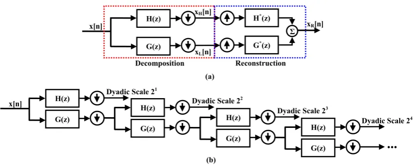
To implement the à trous wavelet transform

algorithm, filters H(z) and G(z) should be used according to the block diagram represented in Fig. 1, [10, 62-63]. According to this block diagram, each smoothing function (SMF) is obtained by sequential

low-pass filtering (convolving with _H(_z2k) _filters), while after high-pass filtering of a SMF (convolving with _G(_z2k) _{filters), the corresponding DWT at} appropriate scale is generated.

For a prototype wavelet ψ(t) with the following quadratic spline Fourier transform,

4

4 ) 4 ( sin )

( _⎟⎟

⎠ ⎞ ⎜⎜

⎝ ⎛

Ω Ω Ω =

Ω j

Ψ (6)

The transfer functions H(z) and G(z) can be obtained from the following equation

(

)

(

sin( 2)

)

4 ) (

) 2 cos( )

(

2

3 2

ω ω

ω ω

ω ω

j j

j j

je e

G

e e H

= =

(7)

and therefore,

( )

[ ]

1 8 { [ 2] 3 [ 1] 3 [ ] [ 1]} [ ] 2 { [ 1] [ ]}

h n

n n n n

g n n n

δ δ δ δ

δ δ

=

+ + + + + −

= + −

(8)

It should be noted that for frequency contents of up to 50 Hz, the à trous algorithm can be used in different sampling frequencies. Therefore, one of the most prominent advantages of the à trous algorithm is the approximate independency of its results from sampling frequency. This is because of the main frequency contents of the ECG signal concentrate on the range less than 20 Hz [62-63]. After examination of various databases with different sampling frequencies (range between 136 to 10 kHz), it has been concluded that in low sampling frequencies (less than 750 Hz), scales 2λ

(λ=1,2,…,5) are usable while for sampling frequencies more than 1000 Hz, scales 2λ _{(λ=1,2,…,8) contain}

profitable information that can be used for the purpose of wave detection, delineation and classification.

In Fig. 2, several dyadic scales obtained via application of à trous DWT to an arbitrary holter record belonging to the DAY general hospital database are illustrated. As it can be seen, by increment of the dyadic dilation parameter 2λ_{, the high-frequency fluctuations of}

the transform induced by measurement noises are diminished.

2.2 Radial Basis Function Based Support Vector Machine (RBF- SVM) Classifier

In this work, RBF-SVM is implemented as arrhythmias classification method. According to Vapnik formulation [66], if couple (xi,δ(xi)) (in which δ(xi) is class function, i=1,_K,N) describing data elements and their corresponding categories which are linearly separable in the feature space, then

b

φ(x) w

f(x) = T + ₍₉₎

where w is weight vector, b is bias term and the condition f(xi)δ(xi)>0 holds. On the other hand, if train data is not linearly separable in the feature space to find a suitable separating hyper plane, the following constrained optimization problem should be solved

(

)

2 1 1

( , ) 2

. . ( ) ( ) 1

1, ,

N j j T

i i i

CoF C

s t

i N

ξ ξ

δ ξ

=

= +

+ ≥ −

=

∑

w w

x w φ x b

K

(10)

where CoF is a cost function. Upon solving the above constrained optimization problem, separating hyper plane will be obtained. In the above equation, C is called regularization parameter which its value generates a trade-off between hyper plane margin and classification error. ξi is stack parameter corresponds to xi. Introducing Lagrange multipliers as

Fig. 1 FIR filter-bank implementation to generate discrete wavelet dyadic scales and smoothing functions transform based on à trous algorithm. (a) one-step generation of detail coefficient scales and reconstruction of the input signal, (b) four-step implementation of DWT for extraction of dyadic scales.

H(z) G(z)

x[n] _H(z)

G(z)

H(z) G(z)

H(z) G(z) Dyadic Scale 21

Dyadic Scale 22

Dyadic Scale 23

Dyadic Scale 24

...

Decomposition

H(z)

G(z)

x[n] H

*_(z)

G*_(z)

Σ

Reconstruction xH[n]

xL[n]

xR[n]

(a)

(b)

C t s K CoF j N j j j N i j i N j j i j i N j j ≤ ≤ = − =

∑

∑∑

∑

= = = = α δ α δ δ α α α α 0 0 ) ( . . ) , ( ) ( ) ( 2 1 ) ( 1 1 1 1 x x x x x (11)

where K(xi,xj) is kernel function obtained from following equation ) ( ) ( )

( i j

T j i

K x,x =φ x φ x (12)

for example, _{( )=( +1)}λ

j T i j i

K x ,x x x is polynomial

kernel of degree λ and K(xi,xj)=exp

(

−γ xi −xj 2

)

is RBF kernel. In the Eq. 11, if αi >0, xis are called support vectors. In specific cases, if αi =C, xis are bounded support vectors and if 0<αi <C, xis will be called unbounded support vector. The solve the constrained Eq. 11, several approaches can be found in the literature, [66]. After solving Eqs. 10 and 11, the decision function f(x) is obtained as follows

∑

∑

= + = j j j j i i i i K ) ( ) ( ) , ( ) ( x φ x w b x x x f(x) α δ δ α (13)

and margin Λ is obtained as

1 1

( ) ( )i j i j ( , )i j

i j

K

δ δ α α

=

∑∑

Λ

w _{x x x x} (14)

More details about fundamental concepts of SVM can be found in [66].

2.3 Modified Learning Vector Quantization Algorithm

2.3.1 Conventional LVQ

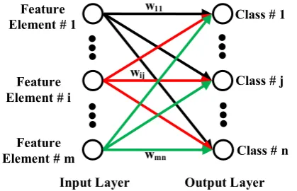
The conventional LVQ algorithm is a learning machine which requires no hidden layer and possesses a m-neuron and a n-neuron input and output layers, respectively. The number of input layer neurons is equal to feature space dimension while the number of output layer neurons is equal to the number of classes forming the feature space. Each neuron of the input layer is attached to all neurons of the output layer via a connection and a scalar weight is associated with each connection (Fig. 3) [67]. The weight between node i of the input layer and node j of the output layer is indicated by wij. According to the LVQ algorithm, to fulfill the train stage, if the k-th input feature vector xk is applied to the network, then an appropriately defined distance of the feature vector with the weights terminating to the j-th output layer neuron is calculated as follows

{

w i m

}

f k j D j i j j k ,..., 2 , 1 ) , ( ) , ( = = = w w x (15)

where f (xi,xj) is a scalar distance function. For instance, f (xi,xj) can be defined as

⎪ ⎪ ⎪ ⎩ ⎪ ⎪ ⎪ ⎨ ⎧ − = ⎟ ⎠ ⎞ ⎜ ⎝ ⎛ ₋ = − − =

∑

∑

= = p k j i j i r p k r j i j i j i T j i j i k k abs p f c k k f b f a 1 / 1 1 )) ( ) ( ( 1 ) , ( ) ( )) ( ) ( ( ) , ( ) ( ) ( ) ( ) , ( ) ( x x x x x x x x x x Σ x x x x (16)

where the first term of the Eq. 16 called generalized distance and for the weight matrix Σ=I the famous Euclidean norm will be achieved. While the second term of the Eq. 16 is called Minkovski distance of degree r and for r=2, again the Euclidean distance appears. The third term of Eq. 16, is called the City Block distance and is used in many pattern recognition cases. If DT(k) indicates an array including distances of the feature vector xkfrom all output layer neurons, then, the label of this feature vector is predicted by the following criterion

(

)

} ,..., 2 , 1 ) , ( { ) ( } ) ( { min ) ( ˆ n j k j D k k k T T = = = D D δ δ (17)

If the predicted label δˆ(k) is true, the minimum distance of the array D_T(k) is decreased by learning rate η proportionally. On the other hand, if δˆ(k) is false, then the minimum distance of the array DT(k) is increased by the same learning rate as [67]

(

)

(

)

(

)

(

)

(

)

min ( )

ˆ

min ( ) min ( ) , ( )

ˆ

min ( ) min ( ) , ( )

T

T T

T T

k

k k if k isTrue

k k if k is False

η δ η δ = ⎧ _{− ×} ⎪ ⎨ + × ⎪⎩ D D D D D (18)

2.3.2 Modified LVQ

Suppose that wij indicates an array including lj scalar weights and the indices i , j are pointers to the i-th neuron in the input and j-th neuron in the output layers, respectively. If each array wij is put into a matrix, the weight matrix

( )

j l p j ×

W will be resulted. In order to formulate the MLVQ algorithm, first it is noted that

c

N

j=1,2,..., shows the class index, Nc is the number of classes and p is the dimension of the feature space. If each column of the weight matrix Wj is indicated by

) (j k

C (k=1,2,...,lj) and fn is a train feature vector, then the distance between fn and all

) (j k

C arrays can be obtained as

(a)

(c)

(e)

(g)

(b)

(d)

(f)

(h)

Fig. 2 Illustration of several DWT dyadic scales 2λ _{obtained from application of a trous filter bank to an arbitrary record of}

high-resolution holter data for (a) λ=1, (b) λ=2, (c) λ=3, (d) λ=4, (e) λ=5, (f) λ=6, (g) λ=7, (h) λ=8.

500 1000 1500 2000 2500 3000

-6 -4 -2 0 2 4 6

Sample Number

N

o

rm

alized

S

ig

n

a

ls

ECG

DWT:21

500 1000 1500 2000 2500 3000

-6 -4 -2 0 2 4 6

Sample Number

N

o

rm

alized

S

ig

n

a

ls

ECG

DWT:23

500 1000 1500 2000 2500 3000

-6 -4 -2 0 2 4 6

Sample Number

No

rm

alized

S

ig

n

a

ls

ECG

DWT:25

500 1000 1500 2000 2500 3000

-6 -4 -2 0 2 4 6

Sample Number

N

o

rm

ali

z

e

d

S

igna

ls

ECG

DWT:27

500 1000 1500 2000 2500 3000

-6 -4 -2 0 2 4 6

Sample Number

N

o

rm

alized

S

ig

n

a

ls

ECG

DWT:22

500 1000 1500 2000 2500 3000

-6 -4 -2 0 2 4 6

Sample Number

No

rm

alized

S

ig

n

a

ls

ECG

DWT:24

500 1000 1500 2000 2500 3000

-6 -4 -2 0 2 4 6

Sample Number

N

o

rm

aliz

ed

S

ig

n

a

ls

ECG

DWT:26

500 1000 1500 2000 2500 3000

-6 -4 -2 0 2 4 6

Sample Number

N

o

rm

a

lized S

ign

als

ECG

DWT:28

) ( ) ( ( ) ( ) ) ( n j k T n j k j kn

d = C −f Σ C −f (19)

where, Σ is a weighting matrix and for Σ=I, the quadratic form is obtained. In this case, the array (j)

n D including all distances between vector fn and

) (j k C s is created. So, the predicted label δˆ _{of feature vector}

n f can be determined as follow

} ,..., { () () 1 ) ( j n j l j n j

n = d d

D (20)

{

min{min( ),...,min( )}

}

ˆ (1) (NC)

n

n D

D δ

δ = (21)

where δ{.} is the associated true label operator of the input argument. If the predicted label is true, then the column (δˆ)

q

C is decreased by learning rate η while if the predicted label is not true, that column is increased by the same learning rate and can be written as

⎪⎩ ⎪ ⎨ ⎧ + = − = = False is if d True is if d d d Arg d n q q q n q q q n n n q δ η δ η δ δ δ δ δ δ δ δ δ δ ˆ ˆ ) ,..., ( min ) ˆ ( ) ˆ ( ) ˆ ( ) ˆ ( ) ˆ ( ) ˆ ( ) ˆ ( ˆ ) ˆ ( 1 ) ˆ ( C C C C (22)

As an interpretation for Eqs. 19 to 22, by inserting feature vector fn, all pre-defined distances between this vector and all weight vectors between input and output layers are calculated and as the result, the fn is considered to belong to the class including minimum distance between all weights and all output neurons. If this classification is true, the minimum distance is decreased by learning rate η while if the outcome of the classification is false, the minimum distance will be increased by η. By this learning strategy, desirable results for the selection of the best weight vector and error increasing rate versus epoch number is attained. The accuracy of the MLVQ network depends upon the following parameters.

The Number of Train Epochs. Generally, more

epoch number results better accuracy and the epochs can be considered to have inverse proportionality with number of weights lj, i.e., the network with larger lj will requires fewer epochs for reaching an acceptable accuracy. Although, a trade-off between the number of

j

l and epochs number can be found.

The Number of Weights Assigned to Each

Connection. In the conventional LVQ method if the

number of train data is a large value, therefore, the weights lying in connections should adapt themselves with several data types and probable outliers and therefore, a weak performance might be expected. To solve this problem, more weights can be assigned to each connection. To this end, one way is to increase the number of the output layer neurons and considering more than one node for each class. Although, by this modification the overall accuracy of the network may increase, however, a malformed topology is obtained. As the second way, instead of assigning a scalar weight

to each connection, a vector including some weights is considered between each input-output neurons connection.

As final comment for the MLVQ method, if a priori probabilities associated with the feature space classes are not equal, in regulation of the weight vector ending to the class with maximum probability, the corresponding neuron of this class will win predominatingly and correspondingly the winning Euclidean norm is permanently decreased and therefore, after passing a large number of train data from the network, in the test stage, inputted features will falsely being guided to this node and consequently the cumulative accuracy is corrupted. To solve this problem, a modified learning rate is proposed as follow

ˆ

1 ( )

ˆ

1 ( )

m L m m L M M

if k is True

M M

M M

if k is False

M M η δ η η δ ⎧ ⎛ ₋ ⎞ ⎪ ⎜ ⎟ ⎪ ⎝ ⎠ = ⎨ ⎛ ⎞ ⎪ ₋ ⎜ ⎟ ⎪ _{⎝ ⎠} ⎩ (23)

where, M, Mm and ML are the number of the train data,

data number of the largest and data number of the smallest classes, respectively.

3 ECG Events Detection and Delineation

Algorithm via Modified Wavelet-Based Algorithm, [63] (summary)

If the discrete wavelet transform of the ECG signal is calculated using a′ trous algorithm, five number of transforms will be obtained for scale values of

5 , 4 , 3 , 2 , 1 ,

2λ λ= _{. The proposed measure of the [63]} study was developed based on simple mathematical calculations. In summary, it was supposed that a rectangular window of length L samples is slid sample to sample on the signal. Therefore, the signal located in the window in k-th slid can be obtained as follows

] 2 / : 2 / [ ) (

2 k L k L

k λ =Wλ − +

Y ₍₂₄₎

where Yk(λ) is a vector including the elements number k to k+L of the scale 2 . To define a new λ measure, the area under the absolute value of the curve

) (λ k

Y and the curve length of Yk(λ) is obtained as

Feature Element # 1

Feature Element # i

wij

Feature Element # m

Class # 1

Class # j

Class # n

w11

wmn

Input Layer Output Layer

Fig. 3 A m×n MLVQ network topology for a

m-dimensionality feature space and n-type categories.

(a) (b)

(c)

(a) (b)

(c)

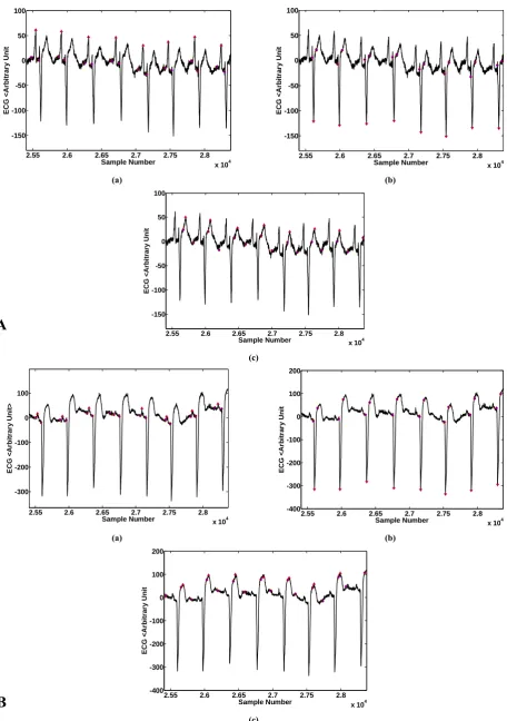
Fig. 4 An excerpted segment from a total delineated ECG. Delineated (a) P-waves, (b) QRS complexes and (c) T-waves. (Circles: edges of event, Triangles: Peak of events, Panel A: lead I, Panel B: lead II).

2.55 2.6 2.65 2.7 2.75 2.8 x 104 -150

-100 -50 0 50 100

Sample Number

ECG <

A

rb

it

ra

ry

Un

it

2.55 2.6 2.65 2.7 2.75 2.8 x 104 -150

-100 -50 0 50 100

Sample Number

EC

G

<

A

rb

it

ra

ry

U

n

it

2.55 2.6 2.65 2.7 2.75 2.8 x 104 -150

-100 -50 0 50 100

Sample Number

ECG

<

A

rb

it

rary

U

n

it

2.55 2.6 2.65 2.7 2.75 2.8 x 104 -300

-200 -100 0 100

Sample Number

EC

G

<

A

rb

it

ra

ry

U

n

it

>

2.55 2.6 2.65 2.7 2.75 2.8 x 104 -400

-300 -200 -100 0 100 200

Sample Number

E

C

G <Ar

b

itr

a

ry

U

n

it

2.55 2.6 2.65 2.7 2.75 2.8 x 104 -400

-300 -200 -100 0 100 200

Sample Number

E

C

G

<

A

rb

it

ra

ry

Un

it

A

B

∫

∫

+ = =

fk t

k

t k

fk t

k t k

dt t y k

Curve

dt t y k Area

0 2 0

) , ( 1 ) (

) , ( )

(

λ λ

& (25)

where t0k and tfk are respectively the start and

beginning points of the vector Yk(λ) and the variable )

, (t λ

yk represents the samples existing in the vector

) (λ

k

Y . Accordingly, the new measure named Area-Curve Length (ACL) is defined as follows

) ( )

( )

(k Areak Curvek

ACL = × (26)

The most significant reason for the definition of the ACL measure according to Eq. 26 is its capability in the detection of ECG wave edges (onset and offset locations).

ACL reaches its minimum value when both the value of the signal Yk(λ) and the corresponding derivative in the window is the least. Therefore, ACL is a measure the minimum value of which is an indicator of minimum amplitude and minimum slope events. This can be observed in wavelet transform scales (See Fig. 2). More details will be available via [63]. In Fig. 4, a graphical representation of the wave detection-delineation algorithm performance on a noisy ECG trend including severe arrhythmia is shown.

4 Design of Premature Contractions (Ventricular, Atrial) Classifier

A new algorithm is aimed to be developed in this part for premature contraction discrimination of atrial, ventricular or both complexes from normal ones based on two-lead ECG data. To meet this end, Holter data gathered in the DAY general hospital2 _{were arranged in}

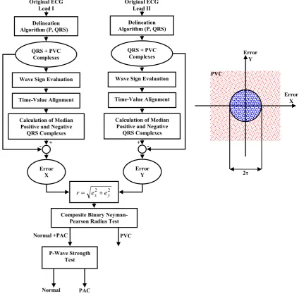
three different groups. First group included only PVCs, second group was only consisted of PACs and the third group was a mixture of PVC and PAC complexes. It should be noted that there is a very significant difference between the morphology of PVC complex and a normal complex (Fig. 5-a). On the other hand, a PAC complex has a morphology very similar to that of a normal complex (Fig. 5-b). Correspondingly, based on a Composite Binary Neyman-Pearson Radius test, the detection algorithm classified the detected complexes into two groups; PVC complexes and a combination of PAC and normal beats. In the next step, in order to distinguish PAC beats from normal complexes, an appropriate measure is defined based on wavelet transform of the delineated P-wave namely as P-Wave

2 _{The high-resolution MEDSET}® _{holter database of DAY general} hospital contains 24-hour 3-lead records of about 150 patients including diverse ECG arrhythmias such as bundle branch blocks, PVC, PAC, myocardial infarction, heart failure, ischemia and T-wave alternans. The sampling frequency of this database is 1000 Hz with 32-bits of resolution. The electrodes of each holter are attached to the subjects chest skin surface at positions 1, 3, 5 via suitable vacuum cups [62-63].

Strength Factor. Accordingly, complexes ensuing a low-power P-wave are assigned as PACs; however, those following a high-power P-wave are specified as normal beats. The block diagram of the proposed ectopic beat isolation algorithm is shown in Fig. 6.

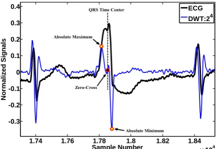
4.1 Time-Value Alignment of the Detected QRS Complexes

In order to time-value alignment of the detected QRS complexes either normal or arrhythmic, first a reliable time center is obtained for each QRS complex. To find this point, the absolute maximum and the absolute minimum indices of the excerpted DWT dyadic scale 24 _{using the onset-offset locations of the}

corresponding QRS complex, are determined. It should be noted that according to comprehensive studies fulfilled in this research, the best time center of each detected QRS complex is the mean of zero-crossing locations of the excerpted DWT (see Fig. 7). After localization of the QRS complex time center, its voltage

(a)

(b)

Fig. 5 A delineated ECG trend [63] including normal

complexes and (a) a PVC with a retrograde conduction into atrium (Rk Rk+1 > Rk-2 Rk-1) and (b) a PAC with delayed sinus

node reset (Rk Rk+1 > Rk-2 Rk-1).

7000 7500 8000 8500 9000 9500 10000 -1500

-1000 -500 0 500 1000 1500 2000

Sample Number

EC

G

<

A

rb

it

ra

ry

U

n

it

>

Rk-1

Rk-2 Rk Rk+1

3.6 3.65 3.7 3.75 3.8 3.85 3.9 x 104 0

500 1000 1500

Sample Number

E

C

G <A

rb

itr

a

ry

U

n

it>

Rk+1

R_k+2 Rk

R_k-1 R_k-2

is subtracted from the QRS complex voltage and in this way, the value of each aligned QRS complex is zero in its time center. In order to find the median waveshape of each lead, appropriate sample numbers toward left and right sides of the QRS complex time center are excerpted and the obtained time-series is put into the signal matrix X in a row-wise fashion. After putting all time-value aligned complexes into the matrix X, in order to find the median waveshape of each lead, the median value of the n-th column of matrix X is assigned as the n-th sample value of the median waveshape. It should be noted that the calculated median waveshape in this way, is more similar to the waveforms with uttermost repetition. In other words, if there is one PVC per three normal complexes, the obtained median waveshape will more resemble to the normal beats.

4.2 Design of PVC Detection Algorithm: Composite Binary Neyman-Pearson Radius Test

In this section, in order to generalize the application of the proposed algorithm, it was applied to 24-hour Holter data of 20 under study subjects of the DAY general hospital. The proposed algorithm can be mentioned as a semi-unsupervised classification method which may be useful in the detection of heart arrhythmias. The most important advantage of an unsupervised classification method is that opposed to an ordinary training method, it is not necessary for data to have label. The structure of the NPC method is so that by using the QRS geometrical properties and P-wave power as proficient features, the type of the detected complex can be specified with acceptable accuracy and low computational load.

Fig. 6 General representation of detected complexes classification on the basis of Composite Binary Neyman-Pearson Radius Test (separation of PVC beats from PAC+normal beats) and P-wave strength test (separation of normal complexes from PAC beats).

Delineation Algorithm (P, QRS)

Wave Sign Evaluation

Calculation of Median Positive and Negative

QRS Complexes QRS + PVC

Complexes

+ Original ECG

Lead I

Error X -

Delineation Algorithm (P, QRS)

Wave Sign Evaluation

Calculation of Median Positive and Negative

QRS Complexes QRS + PVC

Complexes

+ Original ECG

Lead II

Error Y

-

Composite Binary Neyman-Pearson Radius Test

Normal +PAC PVC

Time-Value Alignment Time-Value Alignment

2 2

y

x e

e

r= +

Error X Error

Y

2τ

PVC

P-Wave Strength Test

Normal PAC

Fig. 7 Determination of the time center of a detected QRS complex using excerpted DWT scale 24_.

An appropriate technique is aimed to be developed for discrimination of normal ventricular contractions from abnormal cases. The proposed algorithm can be mentioned as a semi-unsupervised classification method which may be useful in the detection of heart arrhythmias. The most important advantage of an unsupervised classification method is that opposed to an ordinary training method, it is not necessary for data to have label. The structure of the NPC method is so that by using the QRS geometrical properties and P-wave power as proficient features, the type of the detected complex can be specified with acceptable accuracy and low computational load.

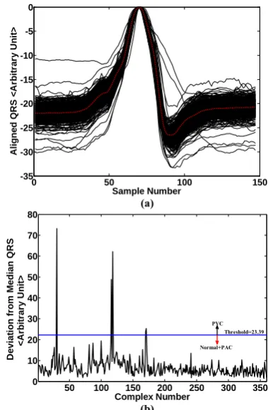
Thus, among all available Holter data, those including only PVC occurrence have been selected. Unless otherwise, other arrhythmia would affect the results of the algorithm and validation procedure will turn to a difficult task. From each subject, 2-chest lead signals were first extracted and QRS complexes were delineated using the previously proposed method. It should be noted that the proposed detection-delineation algorithm detects a combination of normal and PVC complexes, as illustrated in Fig. 6. In the next step, detected complexes were aligned and for each lead a median QRS waveshape was calculated (see Fig. 8-a) and subtracted from each QRS complex. Finally, the resulted error was used in the composite binary Neyman-Pearson radius test [65] and complexes were divided into "normal" and "PVC" categories. Suppose that errors x and y are resulted from subtracting median QRS waveshape from the kth QRS complex. Two hypotheses are first defined as

1 2

1 2

.1: ( , ) ( , )

.2 :

( , ) ( cos( ) , sin( ) ) Hypo

X Y Hypo X Y

ε ε

η θ ε η θ ε

=

= + +

(27)

where, η is a positive constant, θ is a uniformly-distributed random variable in [0,2π], and ε1,ε2 are

independent normal random variables with mean value

of zero and variance of _σ2_{which are also independent}

from θ.

If the observation set is represented as )

, ( ) ,

(X Y = x y ; therefore, the distance between the observation set and origin (0,0)is equal to

2

2 _y

x

r= + . If the radius r is chosen small enough, then Hypo.1 will be held; however, for values of r larger than a specific value, Hypo.2 would be the true hypothesis.

For two independent normal random variables X and Y with the mean value of zero and variance of _σ2_{, the}

resulted random variable R= X2+Y2 will have the following Rayleigh density

⎟ ⎟ ⎠ ⎞ ⎜ ⎜ ⎝ ⎛ −

= ₂ 2₂

2 exp )

(

σ σ

r r

r

fR (28)

In order to design an α-level Neyman-Pearson test, the false-alarm probability should be set to a value and accordingly the appropriate threshold is obtained, [65]. Suppose that false-alarm probability is defined as,

α = =

Γ

∫

_Γ

1 1

0( ) p (yHypo.0)dy

P _Y (29)

Therefore, this equation is an integration of the density fR(r) over the interval [τ,+∞] as follows

2

2 2

2

2

( ) exp

2

exp 2

R

r r

f r dr dr

τ τ σ σ

τ _α

σ

+∞ +∞ ⎛ ⎞

= _⎜− _⎟

⎝ ⎠

⎛− ⎞ = − ⎜ ⎟=

⎝ ⎠

∫

∫

(30)

Solving the above equation, following relation will be resulted for threshold τ in terms of parameters σ and α ,

) ln( 2σ2 α

τ = − (31)

Thus, decision rule of the binary Neyman-Pearson radius test has the following structure,

2 ( )

2 ln( )

NP

PVC r

r

Normal r τ δ

τ

τ σ α

> ⎧

= ⎨ _<

⎩ = −

(32)

where α represents the level (false-alarm probability) of the binary Neyman-Pearson radius test and is chosen arbitrarily as 0.005≤α≤0.05, [65]. It should be noted that although Eqs. 31 and 32 was derived based on simplifying assumptions (independent samples, identical distribution, etc.); however, similar to derivation of Kalman filtering equations, its operation depends only on the first and second-order moments of the signal. Consequently, it can be easily implemented in actual cases and a high performance would be resulted from the algorithm in practical applications, [65]. First hypothesis is according to the situation in which the QRS under study has a slight deviation from median QRS waveshape; however, the second

1.74 1.76 1.78 1.8 1.82 1.84

x 104 -0.3

-0.2 -0.1 0 0.1 0.2 0.3 0.4

Sample Number

N

o

rm

alized

S

ign

als

ECG

DWT:24

Absolute Maximum

Absolute Minimum Zero-Cross

QRS Time Center

hypothesis states that there is a significant difference between the morphology of QRS under study and median QRS. This can more likely be a sign of the existence of PVC. In this study, to find appropriate value of the standard deviation σ , median QRS is subtracted from each detected QRS complex and mean value of the resulted error is then calculated. Afterwards, standard deviation of the error trend is simply calculated and assigned as the appropriate value of σ . The framework of the QRS discrimination algorithm presented in this study is developed based on two ECG leads and correspondingly has less error in comparison to the single-lead algorithm. The algorithm was applied to 24-hour Holter data of 20 subjects including only PVCs and results of validation of the algorithm based on CHECK#1 and CHECK#2 approaches are presented in Table 1. As a result, the average values of 99.43% and 99.32% were obtained for sensitivity and positive prediction, respectively. One of the merits of the proposed algorithm is the simplicity of its implementation in practical cases. An example of the resulted error signal _{r= x}2_+y2 _{(in an arbitrary unit)}

and threshold obtained from Eqs. 31-32 is illustrated in Fig. 8-b. It should also be noted that the QRS complexes with error values above the threshold will be specified as PVCs.

4.3 Separation of Normal Beats from PACs : P-Wave Strength Factor (PSF)

In order to separate normal complexes from PAC's, a new measure called P-wave Strength Factor (PSF) is defined as follows. Assume that the wavelet transform of the detected P-wave is represented as

] : [

2 onk offk

k Wλ P P

U = where k

on

P and k off

P are the start and end locations of the k-th P-wave respectively and

λ

2

W is a vector consisting of DWT of the original ECG in scale 2λ_{. The PSF measure which is similar to the}

signal power criterion is defined for P-waves as

(

)

2 2

) ( )

(k = =

∑

U i

PSF Uk k (33)

Large values of SF represent the existence of strong P-waves; however, small values of SF indicate the occurrence of weak P-waves. Therefore, the decision rule, δPAC, can be defined as follows,

⎩ ⎨ ⎧

> < =

P P PAC

k PSF Normal

k PSF PAC

k

τ τ δ

) (

) ( )

( (34)

where, τPis the decision threshold which can be

considered as τP =μSF −αrσSF with the standard

deviation and mean value of the PSF trend equal to σSF

and , respectively. The parameter αr is threshold

coefficient and can be chosen as 1≤αr ≤3.

In order to determine the appropriate value of the regulation parameter αr, first, about 500 beats

including normal and PAC complexes are selected from all 11 24-hour holter records and for each of them, the PSF is calculated. Then, the obtained PSFs are put into a vector called YPSF and the sample mean (μSF) and the sample standard deviation (σSF) values of the array

PSF

Y are numerically calculated. After calculation of the SF

μ and σSF, a threshold with the structure

SF r SF

p μ α σ

τ = − is considered and using a computer program, the parameter αr is altered from -10 to +10 with the increment step Δα =0.001 . During each increment, the labels of the train set are predicted and the isolation accuracy of the method is calculated. Computerized assessments show that if the parameter

r

α is chosen as to be 1≤αr≤3, the accuracy of algorithm is uniformly maximum and therefore the interval [1 , 3] is the optimum choice for the parameter

r

α . It should be noted that the major PSF characteristic arises from the P-wave morphology during occurrence of the PAC beat. In this case, by incidence of a PAC beat, the distance of the ectopic beat from the previous R-peak is shorter than the median ST/T segment and therefore the P-wave of the ectopic beat may form a fusion with the previous T-wave and the computer program will detect a very short-length P-wave for the premature beat which associated PSF value will be much lower than the other normal complexes.

(a)

(b)

Fig. 8 (a) Time-Value aligned QRS complexes (black) and median QRS waveshape (red), (b) A sample error signal as a tool for PVC classification and the corresponding threshold.

SF

μ

0 50 100 150

-35 -30 -25 -20 -15 -10 -5 0

Sample Number

Alig

ne

d QR

S

<

A

rb

it

ra

ry

U

n

it>

50 100 150 200 250 300 350 0

10 20 30 40 50 60 70 80

Complex Number

D

e

v

ia

ti

on fr

om

Me

dia

n

Q

R

S

<A

rb

itr

a

ry

U

n

it>

PVC Threshold=23.39

Normal+PAC

5 Results and Discussions

5.1 Implementation of the Proposed Method to Long-Duration Holter ECG

A delineated segment of the ECG signal including a PAC complex is illustrated in Fig. 9 with the corresponding wavelet transform in the scale 24_{. As can}

be seen in this figure, for normal complexes, the wavelet transform of the P-wave will have significant oscillations (large SF); however, for PAC beats, very slight movements are observed in the wavelet transform of the P-wave (small SF). An example of the SF trend corresponding to P-waves is depicted in Fig. 10. For values of SF below the threshold of 7.65, the complex is assigned as PAC; however, for SF value greater than the threshold value, it will be specified as a normal complex. To validate the performance of the presented algorithm, it was applied to ECG data including more than 1,500,000 beats and the CHECK#1 and CHECK#2 approaches were used. Finally, the average values of 99.73% and 99.58% were achieved for sensitivity and positive prediction, respectively, which are acceptable results based on reports received from the cardiologists of the DAY general hospital. As a merit of the presented algorithm, it only applies first and second moments of the signal; therefore, it can easily be implemented in practical cases including implantable devices. Results of validation and evaluation of the proposed algorithm are presented in Table 1.

(a)

(b)

Fig. 9 (a) a delineated ECG trend including a PAC (b)

corresponding DWT of the excerpted signal (green triangle: onset of P-wave, red triangle: end of waves).

Fig. 10 P-wave strength factor trend and calculated threshold to separate normal beats from PACs.

5.2 Validation of the Proposed Method 5.2.1 Evaluation of the Selected Features

Discriminant Property

As the first step of the validation, the discriminant power of the(σ_i1,σ_i2,PSF_i)feature vector, in which

2 1, i i σ

σ are the error standard deviations from lead I and lead II templates, respectively and PSFi indicates the mean P-wave strength factor of the beat number i. To this end, first a MLVQ classifier is designed in which the feature space consists of segmented QRS complex (Fig. 11-a), its corresponding dyadic DWT scale 24 _(Fig.

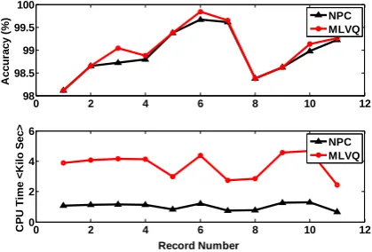
11-b) and RR interval of the beat with the previous and the next R peaks (Fig. 11-c) [68]. It should be noted that, by this feature selection approach, the original QRS waveform with its corresponding DWT dyadic scale and the RR-interval are used as the feature elements, therefore, no ambiguity is increased because no dimensionality reduction method of the QRS complex is employed. Although, the original QRS waveform may be sufficient for getting acceptable results, but adding the corresponding DWT dyadic scale can improve slightly the accuracy of the classification method. The resulted MLVQ classifier is a reliable framework for evaluating another MLVQ classifier tuned with the (σi1,σi2,PSFi) feature vectors. The results obtained from two rival classifiers are compared in Table 2. The graphical representation of Table 2 is shown in Fig. 12. In this table, the summarized results i.e., the CPU time and the accuracy of two MLVQ classifiers applied to two abovementioned feature spaces are shown. As it can be grasped, the mean CPU time and accuracy of the MLVQ classifier with full dimension feature space are 3.717 × 103 _{sec and 99.30%}

while these values are 1.029 × 103 _{sec and 99.26% for}

the newly defined three-dimensional feature space showing rather superiority of the PSF-based MLVQ classification algorithm.

3.5 3.55 3.6 3.65 3.7 3.75 3.8 3.85 x 104 0

500 1000 1500

Sample Number

E

C

G

<

A

rb

it

ra

ry

U

n

it

>

3.5 3.55 3.6 3.65 3.7 3.75 3.8 3.85

x 104 -2000

-1500 -1000 -500 0 500 1000 1500 2000

Sample Number

D

W

T <A

rb

it

ra

ry

U

nit>

50 100 150 200 0

5 10 15 20 25 30 35

Complex Number

P-Wa

v

e

SF

P-Wave SF Threshold = 7.65

Normal

PAC

(a) (b)

(c)

Fig. 11 Extraction of the geometrical features from a delineated QRS complex via segmentation of each complex into 8 polar sectors by generating of a virtual image from the complex. (a) original ECG, (b) DWT of the original ECG and (c) RR-interval.

Fig. 12 Accuracies and CPU times associated with NPC and MLVQ algorithms.

5.2.2 Evaluation of the Neyman-Pearson –Based Classification (NPC) Method

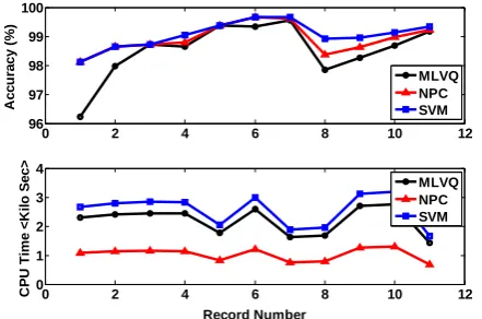
In this case, to evaluate the performance of the NPC algorithm, two classifiers namely as a MLVQ and a SVM are regulated with the (σi₁,σi₂,PSFi) feature vectors. The block-diagram of this step is illustrated in Fig. 13. The obtained results are compared via Table 3. Graphical visualization of Table 3 is depicted in Fig. 14. As a brief explanation for this table, the PAVDAT 9-12

record of the holter database, includes 197,591 QRS complexes which 1153 PVCs and 219 PACs were identified by the MEDSET holter analyzer software. By applying the C++/MEX computer program of the NPC algorithm using a PC system with 2.4 GHz dual core intel CPU with 4 MB cash and 2.0 MB RAM memory, the elapsed time was about 17.15 min while the run – time for the MLVQ and SVM algorithms were about 36.56 min and 42.34 min, respectively.

As it can be seen, in spite of the much lower computational burden imposed by the NPC approach, the proposed discrimination algorithm yields acceptable average accuracy versus the MLVQ and the SVM classifiers.

5.2.3 Global Accuracy Assessment of the Proposed NPC Learning Machine

As the final step of the validation procedure, a SVM classifier with a new feature space is tuned as described. Each QRS region and also its corresponding DWT are supposed as virtual images and each of them is divided into eight polar sectors. Next, the curve length and the polar area of each excerpted segment are calculated and are used as the elements of the feature space, (therefore, for each detected QRS complex, 32 features are computed). A generic example of a holter ECG and its

1.74 1.76 1.78 1.8 1.82 1.84

x 104 0.7

0.8 0.9 1 1.1 1.2 1.3

Sample Number

N

o

rm

ali

z

ed S

ignal

x y

φ_R φ_L

6 5 8

4 3 2

1

7 Normal

Normal PVC

1.74 1.76 1.78 1.8 1.82 1.84

x 104 -0.5

-0.4 -0.3 -0.2 -0.1 0 0.1 0.2 0.3 0.4

Sample Number

N

o

rm

al

iz

ed S

igna

l

Normal

Normal PVC

x y

φR

φ_L

1 4

2 3

5 8

6 7

1.72 1.74 1.76 1.78 1.8 1.82 1.84

x 104 0.8

0.9 1 1.1 1.2 1.3

Sample Number

N

o

rm

al

iz

ed S

ig

n

al

R_k+1 R_k-1

R_k

RR_k RR_k+1

0 2 4 6 8 10 12 98

98.5 99 99.5 100

Ac

c

u

ra

c

y

(%

) NPC

MLVQ

0 2 4 6 8 10 12 0

2 4 6

Record Number

CP

U T

im

e

<

K

il

o

S

e

c

>

NPC MLVQ

corresponding 24 _{DWT dyadic scale with the virtual}

images of the complexes provided for feature extraction are shown in Fig. 11. In Fig. 15 the general block diagram of the ECG beats annotation algorithm with the proposed QRS geometrical feature space is illustrated. According to this figure, first the original ECG is pre-processed and then the QRS complexes are detected and delineated. Afterwards, the proposed geometrical method is applied to the delineated complexes and the feature vectors associated with corresponding complexes are generated. The performance of the SVM classifier with the efficient feature space is compared with the newly proposed PSF-based NPC in Table 4. As it can be seen, the performance of the SVM classifier is partly superior rather than the PSF-based NPC but at the expense of much higher computational burden.

Delineation Algorithm (P, QRS)

Wave Sign Evaluation

Calculation of Median Positive and Negative QRS Complexes

QRS + PVC Complexes

+

Error X

-Delineation Algorithm (P, QRS)

Wave Sign Evaluation

Calculation of Median Positive and Negative QRS Complexes

QRS + PVC Complexes

+

Error Y

-Time-Value Alignment Time-Value Alignment

P-Wave Strength

Factor Std(.) Std(.)

P-Wave Strength Factor

MUX

MLVQ or SVM Classifiers

Predicted Labels

Fig. 13 The block diagram of the algorithm used for selected features discriminant quality evaluation.

Fig. 14 Accuracy and CPU time comparison of the MLVQ,

NPC and SVM classifiers given a common train-test feature space.

Original ECG

Scale 2λ

λ=1,…,6

Reliable QRS Detection-Delineation Algorithm Discrete Wavelet Transform

Generating Virtual Image from the Original ECG

QRS Edges and RR-Tachogram

QRS Close-up Parameters

Segmentation

Curve Length and Polar Area Resampling into Frequency 1000 Hz

Feature Space (Dimension=34)

Classification Algorithm Feature Extraction

Classification Predicted Labels

Test & Train Datasets

Fig. 15 The general block diagram of a ECG beat type

recognition algorithm supplied with the virtual image-based geometrical features.

Fig. 16Global accuracy and CPUT comparison of the QRS

geometric-based SVM and PSF-based NPC learning machines.

To provide a graphical feasibility for achieving a better realization from Table 4, in Fig. 16, the accuracies and CPUT of two SVM and NPC algorithms are plotted.

6 Conclusion

The major aim of this study was to categorize the QRS complex of the high sampling frequency long-duration holter electrocardiogram signal via a simple mathematically originated discrimination algorithm into three Normal, PAC and PVC clusters. The

0 2 4 6 8 10 12 96

97 98 99 100

A

ccu

ra

c

y

(%

)

MLVQ NPC SVM

0 2 4 6 8 10 12 0

1 2 3 4

Record Number

C

P

U

T

im

e

<K

ilo

S

e

c>

MLVQ NPC SVM

0 2 4 6 8 10 12 98

99 100

A

ccu

racy (

%

) NPC

SVM

0 2 4 6 8 10 12 0

2 4

Record Number

C

P

U Ti

m

e

<

K

il

o S

e

c

>

NPC SVM

categorization of the aforementioned beat types is an important subject in the determination of the templates associated with Normal, PAC and PVC beats assisting the physicians to diagnose the heart disease of patient. Because of the fact that the holter signal recorded during 24 hours has a huge number of samples (approximately 86,000 beats), if the classification algorithm has a sophisticated and complicated structure, the computational burden imposed by the computerized implementation of the algorithm may be so heavy that may make impossible processing and classification of all delineated beats. In this study, a method was proposed which its operational complexity was at a low level along with acceptable performance accuracy. By introducing the proposed method, it was evaluated that the method can be applied to very long-duration holter database to identify the Normal, PAC and PVC complexes. The processing speed of the proposed algorithm is more than 176,000 samples/sec as well as average sensitivity Se=99.73% and average positive predictivity P+=99.58% showing desirable performance

in the area of the heart arrhythmia classification. The performance of the proposed two-lead NPC algorithm is compared with MLVQ and SVM classifiers and the obtained results indicate the validity of the proposed method. On the other hand, to justify the newly defined feature space (σi1, σi2, PSFi), a NPC with the proposed

feature space and a MLVQ classification algorithm trained with the original complex and its corresponding DWT as well as RR interval are considered and their performances were compared with each other. An accuracy difference about 0.04% indicates remarkable discriminant quality of the properly selected feature elements.

Acknowledgement

The authors wish to dedicate sincere thanks to Professor Jami G. Shakibi (director of DAY general Hospital NICEL) and Professor Reza Rahmani (director of Imam Khomeini Hospital Catheter Lab.) for their lively discussions during evolution of this study.

Table 1 Performance evaluation of the pro