International Journal of Social Science and Economics Invention
ISSN: 2455-6289
Original Article
Appraising the Impacts of Globalization on Gravity
Model Economic Systems
Dr. Bilal Khlaf Al.Omari
Assistant Professor in Economics, Al.Buraimi University College, Department of Business Administration & Accounting
Corresponding author - Dr. Bilal Khlaf Al.Omari, bilal
@
buc.edu.om
Received 02 September 2019; Accepted 11 September 2019; Published 17September 2019
Abstract
This study aims at exploring the impact of economic globalization factors on the gravity economic systems. Nonetheless, the basis of the research is a gravity economic system exposed to the impacts of globalization, and the concern is to explore the effects of the exposure on the influences of distance and economic sizes on the model. Recognizing the role of population growth and globalization in driving bilateral trade follows is one of the objectives of this research as should be part of an economic model. The study used the modified gravity and globalization variables, data retrieved from the CEPII, the World Fact-book, and the World Bank. The ordinary squares regression and STATA statistical software were used to investigate the hypotheses. The model leading to the general hypothesis that globalization is reducing the cost of entry, and total time required to set up a business and to minimize the bureaucracy associated with registering businesses and launching operations. The trade flow latent variable should contain information on export, import, free trade agreements, preferential trade agreements, and union memberships, which would help in identifying globalization factors that mediate the interaction between global variables and bilateral trade responses.
Keywords:Gravity Model, Globalization, International Trade, Bilateral Trade and Free Trade.
Introduction
Economic development has been one of the critical determinants of human development, and since the onset of industrial and agrarian revolutions, humanity has achieved significant milestones. Most of the achievements have been geared towards obtaining and sustaining a global community accessible without the spatial and temporal restricts. It suffices to deduce that globalization has spearheaded such endeavours and it has immense contribution to international trade developments and another related aspect. However, one of the commonly used and numerically robust models, the gravity model, is yet to consider the effects of globalization on related systems and to explore and account for the influence of economic globalization factors on the gravity economic systems.
Globalization is arguably the mainstay of economic growth and prosperity in the contemporary global environment. Despite its complications and intricacies, globalization influence economic, social, environmental and political aspects of life. In the context of economic globalization, some of the dormant benefits include but not limited to reduced trade barriers and tariffs, improved flow of goods and services as across national boundaries, and the ease of migration due negotiated and improved international affairs and relations among countries (Samimi & Jenatabadi, 2014). It is clear that globalization has played a significant part in the evolution of international economics and it suffices to deduce that it has contributed to preceded development in some of the conventional
constructs and principles in innumerable ways. Further, globalization has influenced bilateral trade and its predictors.
Literature Review
is reliable and robust evidence supporting the relationship between bilateral trade and primary determinants such as distance and economic size of the trading countries (Chaney, 2018). However, it is imperative to note that Chaney‟s work was focused on understanding and establishing the role of the distance between two countries with existing bilateral agreements.
Of concern is the role that globalization plays in delimiting some of the factors that may have influenced the performance of the gravity model because it is apparent that many operational and technical improvements can be ascribed to economic globalization. The conventional form of the gravity law is a deduction of Newton‟s law of universal gravitation, and it is of the following form:
( ) ( )
( )
The modification in the above equation is meant to give it a global representation in that and represents matrices of paired trading countries and the power indices approximate unity for the gravity equation of international trade to hold. It is also important to reiterate Chaney‟s position that the role of the economic size represented by alpha and beta are well understood except for that of distance (Chaney, 2018). However, this is not to dispute the ability of gravity model over time but rather to explore the likely contribution of globalization in exploring the role of distance on bilateral trade flows. From a historical perspective, globalization has played a role in further joint unions and advocating for favourable global bilateral trades based on common interests. Egger (2002) proposed a new version of the gravity model, even though the modification aimed at forecasting trade potentials between countries. However, it is imperative to note that author relied on the regression residuals as the potential of trade and it represented the difference between actual bilateral trade the potential trade between any pair of countries (Egger, 2002). Egger‟s model suggests that bilateral trade is a function of GDP (referred to as factor income), size of the country (expressed as a proportion of population against GDP), and the differences in endowments. However, it is paramount to note the mode employed additive summation on some of the factors and identified combined effects instead of individual factor effects (Egger, 2002). Further, the model focused on the estimation of bilateral exports.
Elena-Daniela (2012) also estimated a gravity model targeting external trade for Romania using Foreign Direct Investment (FDI) as an additional variable and a modification to the conventional gravity model to suit the objectives of the study. As per the results of the study, bilateral trade between Romania and its partners is dependent on GDP, the distance between the trading partners, FDI, and the existence of common borders (Vioricã, 2012). Other studies have also reached at the same conclusion with the overall inference confirming the direction of the relationship between bilateral trade, distance, and size of the country regarding economics (Kareem & others, 2013; Linders & De Groot, 2006). However, there are additional attributes that can in explaining trade flows between countries.
Bloomberg et al. (2009) conducted a study on the gravity model of globalization, democracy and transitional terrorism but focused on the influence of democratic institutions as well as international integration on non-state economic elements (Blomberg & Rosendorff, 2009). Dias (2010) addressed the effects of distance on international trade and postulated that globalization has an unknown influence on the elasticity of the distance between trading
partners. According to the author, globalization results in reduced cost of trade as well as barriers to production due to the ease of decentralization (Dias, 2011). Other authors who have addressed the globalization and gravity model in different circumstances but it agreed that the impacts of globalization require further research, especially when it comes to its influence on gravity economic systems.
Novelty and Contribution
One of the overarching questions is the representative capacity of the GDP without the inclusion of the population as well as socio-economic status in representing the consumption capacity of a country relative to another. That is, presumably and deservedly so, both GDP and population of the two countries ought to be explanatory variables in the gravity model as opposed to the approach that Egger (2002) took. However, it would also be prudent to compare the two models to establish the best performing an appropriate one. Nonetheless, this study recognizes the role of population growth and globalization in driving bilateral trade flows. For instance, the process of importing cars is not as bureaucratic as it used to be, while also forwarding, clearing, and import duty fees and taxes are far easier to complete due to technology and other synergy and bilateral agreements between countries.
The impact of such improvements, innovations, and developments on bilateral flows should be part of an economic model system. It is vital to note that international trade has under remarkable growth over the last two years and about 25% of global products account for annual exports (Liu & Luo, 2004; Savrul & Insecara, 2015). It is very crucial to understand the factors that have contributed to this process because gains from the growth had benefited countries and stimulated unprecedented economic growth in multiple countries or origins. Even though it may be appropriate to describe the growth to comparative advantage, it is necessary to note that product specialization is not the only driving factor driving growth in international trade. As such, this article postulates a modified gravity model that accounts for the influence of chosen elements of globalization on international trade flows. It is, however, critical to note that data and the mathematical proofs regarding some of these attributes are limited and have not been a focus of numerical studies. Of interest is the fact that many drop shipping companies have penetrated markets that would otherwise be imposed to reach. In this context, the overarching question is whether or not contemporary international bilateral trade models consider the influence of such emerging technologies or not.
Methodology
The ideal regression equation approximating the proposed model aims to measure the flow of bilateral trade between countries and over a defined time. In this case, the proposed bilateral trade agreement is of the form:
2004). The introduction of the globalization variable is the modification made on the gravity equation, and the introduced variables would be discussed in the subsequent sections.
Gravity Variables
Concentrating on gravity variables and different scenarios and modelling parameters have been developed to define different gravity equations. It is virtually possible to find gravity robustness test in all regression analysis in most of the articles, technical papers, and white papers. Against this historical backdrop as well as the tendency to use gravity variables in most articles, the study embraced the universal decision to include the same variables as a means of determining the additional variables that explain the variation in bilateral trade besides the gravity variables.
The main gravity variables consist of distance, common border, cultural distance and economic scales of the partnering countries. Regarding distance Smarzynska (2001) exploited the importance and influence of distance on trade flows and noted that proximity reduces the impacts of distance on bilateral trade. Arguably, proximity reduces costs associated with transport, time lags, product spoilage, and the cost of collecting legal information regarding the existing legal agreements (Smarzynska, 2001). However, many organizations believe that such factors cannot fully explain the variations observed between bilateral trade flows and the primary predictor variables.
Based on the conventional practices, a natural log transformation is necessary before conducting a regression analysis between bilateral trade flow attribute and its explanatory variables. Common border and the related inter-governmental agreement also play an essential in determining the effectiveness of bilateral trade. In most cases, the influence of the distance between bordering countries tends to be non-linear because of the proximity and the ease of transporting, processing, and receiving goods. In general, countries that share borders tend to find it easy and efficient if they share a common border, and the variable is dichotomous.
The other variable of interest and considered a critical component of the gravity variable is the cultural distance. Cultural distance is a function of colonialism and the factional alignments and loyalties. It is imperative to note that Cultural Distance attribute is closely related to standard language indicator, and is also a dichotomous variable assuming the values of 1 for pairing countries that share the same colony as well as language. Notably, the colonial ties have close relations with Colonial Ties, and it is fortunate or unfortunate that both variables measure or approximates the same effect. It is also essential to note that the Colonial Ties variable is also dichotomous and assume a value of 1 for countries that shared the same colony; otherwise, the corresponding value is zero. Nonetheless, it is imperative to note that Colonizer ties have more than one dimension because it is possible to consider past and present colonial affiliations.
Finally, one of the significant gravity variables is economies of scales, and past studies have demonstrated that the log of the production of the GDP of two countries is a useful scale variable for estimating and establishing the influence of GDP on bilateral trade. It is also imperative to note that several studies have included per Capita GDP using discrete means, despite the paper focuses on a more direct approach to understanding its influence on the entire model.
Globalization Variables
It is imperative to note that globalization brought with it currency unions and some exchange rate volatility concerns that have revolutionized bilateral trade flows. As a convention, the variables used in the numerical model have a and designations to note the country of origin and destination country. For ease of understanding an and represents and trading countries and partners.
As a measure that accounts for the influence of population density on bilateral trade flows, the ratio between the areas, and per capita were considered alongside GDP and population of the trading countries proves critical in further assessments. Many attributes have been included to account the influence of globalization such as; population, area of the country, duration differences between imports and exports, homogeny of both origin, destination countries, membership to GATTO, Union Membership, migration from one trading bloc to another, cost of entry into a market, and the required time to successfully launched a business venture. The preceding argument is that globalization has shortened the time required to set up a business, and it has reduced the duration for processing and clearing goods. Furthermore, membership in trading blocs and unions also ease processes of clearing and forwarding goods. From a logistics perspective, the number of players in the airline transport industry has significantly increased, and it is virtually possible to receive an item ordered online within a week or two.
Based on the trends, it suffices to deduce that some of these innovations and developments have modified and changed some of the influences and predictions of the gravity model. For example, proper airline transport networks, protocols, and bilateral agreements, it is possible to reduce transit time through direct flights, and such will influence the effect of distance on bilateral trade between the two countries (De Benedictis & Taglioni, 2011; Lewer & den Berg, 2008). A typical example is the launch of direct flights from Kenya to the United States of America. The direct flight saves the business community over 20 hours of flight time, and about 80% of flight charges and the impact it has on bilateral trade between the US and Kenya imply the gravity model of the two countries. Consequently, it is commanding to explore and understand the consequences of economic globalization initiatives on the gravity model and the long-term implications of such changes and trends in the global economy.
Data Sources
The data used in the study were retrieved from the CEPII website, but the datasets were recovered from different databases. The data consists of 224 pairs of countries, and as such, the attributes cover a global scope. In part, the gravity model data alongside the other variables were reclaimed from CEPII and other sources. The strategy for extracting, transforming and loading the data was based on international standards and country codes defined in the original gravity CEPII data retrieved from CEPII. The source of the data is Head, Mayer, and Ries (2010) and the paper focuses on colonial erosion bilateral related trade agreements. It is imperative to note that the cited paper focuses on monadic and dyadic effects of specific factors on bilateral trade (Head, Mayer, & Ries, 2010). However, the factors are not related to globalization attributes.
The other relevant sources of the data are as follows
available and commences from 1960, which ceases to track countries that terminate the required membership. The reporting on Russian GDP commences in 1989. The other attributes that can be traced to the Head, Mayer, and Ries (2010) article are Free Trade Agreement features and Preferential Trade Agreement. Most of the trading blocs are in pursuit of trade agreements and globalization is playing an essential role in furthering the agenda. The FTA and PTA variables data cover the period 1948 and 2006. The data used in the article was cleaned while the source included variables such as Factual Presentation (FP) and Factual Abstract (FA) with FP distributed, Held, suspended, reported and not reported statuses. Additionally, it is considerable to note that the counts and types of agreements also differed. However, the number of paired countries matched that obtained from the gravity model data and made it easier to understand and merge the datasets. The other datasets retrieved from external sources included independence data from the World Fact-book based on the report that Head, Mayer, and Ries (2010) submitted, currency union data from Jose de Sousa‟s website and the rest data were from Geo-Dist database of CEPII. The Geo-Dist data set had information on the distance between countries, the areas of each of the countries, common language as well as former colonies and related colonial data. Some of the distinct globalization related variables include the cost of business registration and start-up, start-up procedure, the time required to launch start-ups, and time differences between imports and exports.
Model Variables
The variables used in the study can be summarized as follows.
Table 1: Description of Attributes used in modelling the Impacts of Globalization on the Gravity Model
Variable Data Type SI Unit
Independent Variables
Origin Population (oPOP) Numeric Destination Population (dPOP) Numeric
Origin GDP (oGDP) Numeric US dollars Destination GDP (dGDP) Numeric US dollars Per capita oGDP (poGDP) Numeric US dollars Per capita dGDP (pdGDP) Numeric US dollars Distance between countries
(DIST)
Numeric Kilometres
Time Difference (TDIV) Numeric Hours Common Language (COML) 0/1 Dummy Common Currency (COMC) 0/1 Dummy Colony (COL)
Contiguity (CONT) Globalization Indices
Origin Entry Cost (oEC) Percentage (start-up)
% of GNI
Destination Entry Cost (dEC) Percentage (start-up)
% of GNI
Origin Entry Process (oEP) Numeric Count Destination Entry Process
(dEP)
Numeric Count
Origin Entry Time (oET) Numeric Days Destination Entry Time (dET) Numeric Days Dependent Variable
Free Trade Area (FTA) 0/1 RTA =1 otherwise 0
Model Specifications
The premise upon which this paper is based is that of interacting between specific people, groups and dimensions of space, time, per
capita, and population. The study aimed at exploring how human dimensionality principle responds and conforms to the already observed interactions that the gravity model predicts but in the context of globalization. As per the principle, people interact more as they became faster, closer, more significant and empowered to be active from a financial perspective (Bergstrand, 1985; Chaney, 2008). Conversely, people will tend to interact less with increasing distance, smaller population, minimal activities per period, and an increasing number of non-common interest activities. In the context of this study, globalization is a factor that has brought people together and instigated the concept of a global community irrespective of the distance countries and continents.
Instead of interacting, the study focused on bilateral trade and the hypothesis focuses on the factors that determine bilateral trade flows. Of importance is to understand and explore the influence of globalization on the different time aspect of bilateral trade flows between two countries or pairs of countries based on the panel data used in this study. Hence, against a backdrop of this hypothetical discourse, the log version of the modified gravity model that accounts for the effects of globalization on bilateral trade is as shown below: ( ) ( ) ( ) ( ) ( ) ( ) ( ) ( ) ( ) ( ) ( ) ( ) ( ) ( ) ( ) ( )
Hypotheses Related to Model Coefficients
The contribution of each of the factors to bilateral trade as well as the contribution of globalization on the gravity model is dependent on the decision criteria for the regression coefficient for each of the attributes. As stated earlier and in different literature, each of the gravity models tends to have a different relationship with the bilateral trade and of importance is to explore the plausible contribution of globalization on international trade as well as financial performance. Hence, besides the general hypothesis deduced from the principle of interacting, it suffices to emphasize that the inclusion and inclusion criteria for above-declared variables depend on the statistical test of significance for the regression coefficients.
It is impervious to note that modified version of the gravity model considers export, demand, and trade supporting or impeding factors that have a direct association with globalization and its influence on the processes of sealing treaties, accepting trade agreements and signing import and export contracts. Hence, in general, the hypothesis that all the identified variables contribute to bilateral trade flows between the paired countries holds and as such, the coefficients of these variables are different from zero. That is, null hypotheses that the coefficients are equal to zero were tested against the alternative that they were different from zero.
Results and Discussions
obtained. It is paramount to note that including all these variables were aimed at finding those that had a significant contribution to bilateral trade between paired countries.
Given that the study relied on ordinary least squares regression for empirical testing of the model, which leads to note that the approach may have some limitations depending on the data management, and analysis practices deployed during analysis and interpretation. For instance, most of the gravity models do not consider the consequence of heteroskedasticity on the estimated bilateral flows between any pair of trading partners. The concern is on the accuracy of gravity model under heteroskedasticity because the error terms are hardly accounted for and the inequality may become much worse when „exogenous‟ factors such as globalization are included in the model. Furthermore, the gravity model relies on time-series which are prone to non-stationarity issues because refreshing time-series and attempting to retrieve reliable econometrics exposes the analysis to problems such as
random walk. As such, robust regression and necessary correction mechanisms were undertaken to ensure that the results were not affected by either heteroskedasticity or random walk.
Model Results and Interpretations
The statistical evaluation consisted of two distinct phases to evaluate both the conventional and modified gravity models.
Conventional Gravity Model
The conventional gravity model is defined regarding economics scales and distance variables. That is, it is a function of GDP and distance; nonetheless, both attributes are weighted for the population. However, such models do not consider the influence of demand that tends to be a function population and per capita GDP on trade flows. Based on the data used in the study, the results of the conventional gravity model is as shown below.
Table 2: Regression Results assuming that the dependent variable is a binary variable
FTA Coef. Std. Err. z P>z [95% Conf. Interval]
DIST -1.321613 .0048847 -270.56 0.000 -1.331187 -1.312039
COML .7916086 .0106713 74.18 0.000 .7706932 .8125241
CONT .61787 .0194173 31.82 0.000 .5798129 .6559271
oGDP .0835538 .0021792 38.34 0.000 .0792826 .0878249
dGDP .0835538 .0021792 38.34 0.000 .0792826 .0878249
poGDP .4357269 .0034451 126.48 0.000 .4289745 .4424792
pdGDP .4357269 .0034451 126.48 0.000 .4289745 .4424792
COL -.2350492 .0269031 -8.74 0.000 -.2877784 -.1823201
COMC -.7267453 .0217924 -33.35 0.000 -.7694577 -.6840329
Constant -3.244247 .067252 -48.24 0.000 -3.376059 -3.112435
As per the model, all the regression coefficients are statistically significant at 5%. That is, all the p-values are less alpha (0.05), and it suffices to deduce that the gravity model holds based on the results. Additionally, the coefficients of distance variable, as well as the rest of the gravity variable, have proportional directionality that conforms to reports in most literature and research articles. However, Colony and Common Currency attributes exhibit a different relationship with bilateral trade flows. According to Miron, Miclaus, and Vamvu (2013), bilateral trade flow instigates
common currency against the assumption that common currency is one of the factors that account for the flows (Miron, Miclaus, & Vamvu, 2013).
From such a perspective, the deductions made regarding the Common Currency coefficient are sensible. The results of a variant of the model, assuming that the dependent variable is continuous are as shown in Table 3. In this case, the regression coefficients are different in magnitude, and not all of the attributes are statistically significant.
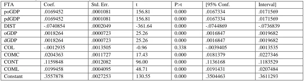
Table 3: The regression results assuming that FTA is a continuous variable
FTA Coef. Std. Err. t P>t [95% Conf. Interval]
poGDP .0169452 .0001081 156.81 0.000 .0167334 .0171569
pdGDP .0169452 .0001081 156.81 0.000 .0167334 .0171569
DIST -.0740854 .0002049 -361.64 0.000 -.0744869 -.0736839
oGDP .0018264 .0000723 25.26 0.000 .0016847 .0019682
dGDP .0018264 .0000723 25.26 0.000 .0016847 .0019682
COL -.0012935 .0013505 -0.96 0.338 -.0039405 .0013535
COMC .0204363 .0011727 17.43 0.000 .0181379 .0227346
CONT .1159848 .0012082 96.00 0.000 .1136168 .1183529
COML .0199458 .0004095 48.71 0.000 .0191431 .0207484
Constant .3557878 .0027253 130.55 0.000 .3504463 .3611293
According to Table 3, Distance and Colony have an inverse relationship with bilateral trade flows, even so, Colony is not a statistically significant factor of international trade. The coefficient of determination for the first model is 0.3584, while the second gravity model is 0.1653. Hence, gravity variables in Table 2 explain about 36% of the variations in bilateral trade flows compared to approximately 17% that the model in Table 3
explains. The difference between the two models should be noted and discussed further.
Modified Gravity Model
colonization and most of the current alliances formed are based on shared interests, especially regarding export and import capacity.
Such influence gravitates around some of the factors that been included in the following model.
Table 4: Logit Regression Model Estimate
FTA Coef. Std. Err. z P>z [95% Conf. Interval]
DIST -1.4171 .0116333 -121.81 0.000 -1.439901 -1.394299
COML .600335 .0160457 37.41 0.000 .568886 .6317841
CONT 1.055228 .0353952 29.81 0.000 .9858549 1.124602
oGDP .0493496 .0034579 14.27 0.000 .0425722 .056127
dGDP .0493186 .003457 14.27 0.000 .0425429 .0560942
poGDP .3320964 .005766 57.60 0.000 .3207952 .3433977
pdGDP .3299397 .0054777 60.23 0.000 .3192036 .3406758
COL -.0349543 .041652 -0.84 0.401 -.1165908 .0466822
COMC -.3032565 .0339904 -8.92 0.000 -.3698765 -.2366364
TDIV -.0715824 .003412 -20.98 0.000 -.0782698 -.064895
oEC .0001089 .0000836 1.30 0.193 -.000055 .0002727
oEP -.0773395 .0023228 -33.30 0.000 -.081892 -.072787
dEP -.0771851 .0023165 -33.32 0.000 -.0817253 -.0726449
oET .0005931 .0001538 3.86 0.000 .0002917 .0008945
dET .0006209 .0001518 4.09 0.000 .0003234 .0009184
Constant 3.022188 .1360486 22.21 0.000 2.755538 3.288839
Based on the probabilities of the coefficients, there is no evidence supporting the claim that Colony and Entry Cost at the country of origin influence bilateral trade flows. However, besides distance, the model suggests that Common Currency, Time Difference,
Entry Process at origin and Entry Process at destination country have an inverse relationship with bilateral trade flows
A similar approach was used to develop an alternative model whose results are presented in Table 5.
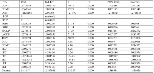
Table 5: Multiple Linear Regression Model Estimate
FTA Coef. Std. Err. t P>t [95% Conf. Interval]
CONT .1776385 .0036172 49.11 0.000 .1705488 .1847281
COML .0361361 .001234 29.28 0.000 .0337175 .0385548
DIST -.2126166 .001003 -211.99 0.000 -.2145824 -.2106508
oPOP 0 (omitted)
dPOP 0 (omitted)
oGDP .0025238 .0002267 11.14 0.000 .0020796 .002968
dGDP .0025238 .0002267 11.14 0.000 .0020796 .002968
poGDP .0274814 .0003856 71.27 0.000 .0267257 .0282372
pdGDP .0274814 .0003856 71.27 0.000 .0267257 .0282372
TDIV .0128894 .0002139 60.27 0.000 .0124703 .0133086
COL .0147458 .0040081 3.68 0.000 .00689 .0226016
COMC .0145027 .0035361 4.10 0.000 .0075721 .0214333
oEC .0000271 4.33e-06 6.26 0.000 .0000186 .0000356
dEC .0000271 4.33e-06 6.26 0.000 .0000186 .0000356
oEP -.0053948 .0001559 -34.61 0.000 -.0057003 -.0050893
dEP -.0053948 .0001559 -34.61 0.000 -.0057003 -.0050893
oET .0000738 9.59e-06 7.70 0.000 .000055 .0000926
dET .0000738 9.59e-06 7.70 0.000 .000055 .0000926
Constant 1.41047 .0107941 130.67 0.000 1.389314 1.431626
Table 5, unlike Table 3, includes an exclusion requirement for model parameters with zero regression coefficients. The population attributes are omitted from the model, despite that it is imperative to note that distance and economic scale attributes were normalized using the population for each of the paired countries.
The coefficient of determination for the first model is 0.3463, while that of the second gravity model is 0.2883. Hence, gravity variables in Table indicate that about 35% of the variations in bilateral trade flows compared to approximately 29% that the model in Table 5 explains the difference between the two models should be noted and discussed further.
Discussion
There are debates on the proper form of gravity model and the empirical results presented in Tables 2 & 3 and Tables 4 & 5 attest to the differences in gravity models developed and the subsequent lack of a universal gravity model. Based on ANOVA tables,
, all the four models are a better fit the panel
essential to note the difference in improvement between the two sets of models.
Specifically, the conventional gravity model obtained from logit regression had an adjusted R-squared of 0.3584 compared to 0.3463 for the modified gravity model. Conversely, the conventional gravity model obtained from the alternative regression had an adjusted R-squared of 0.1653 compared to 0.2883 for the modified gravity model. The logit regression model does show improvement in bilateral trade flows due to the inclusion of globalization factors. On the other hand, the other model shows improvement in the performance of the model with the inclusion of these factors. Besides the increase of adjusted R-squared from 0.1653 to 0.2883, the changes in root mean square associated with model increased from 0.1915 to 0.2694, although the change is smaller compared to that obtained from logit regression results. Hence, the best model parameters discussed and used to lead the discussion on the impacts of globalization is presented in Table 5.
Egger and Pfaffermayr (2003) discussed that bilateral trade flows ought to have a direct positive relationship with economic size measured regarding population and GDP. Further, from literature is expected that population have a negative coefficient if
the exported goods are capital intensive or luxuries goods from the perspective of the destination country (Egger & Pfaffermayr, 2003; Grünfeld & Moxnes, 2003). From a theoretical perspective, a large population is indicative of a large domestic market that also promotes division of labour hence creating opportunities for many goods. From such a perspective, the population should have a positive impact on bilateral trade flows. Other studies have also established that GDP and per capita GDP are reasonable measures of demand and supply for imports and exports respectively (Burger, Van Oort, & Linders, 2009; Feal-Zubimendi, Rosas Garc, Hernaiz, & Bastos, 2018; Gómez-Herrera, 2013). Based on the arguments that the authors present, the coefficients of these attributes ought to be harmful, while other numerical evaluations have produced different results (Marinov et al., 2014). It is also imperative to note that studies that have relied on cross-sectional data have established negative impacts of population on trade flows, although others have established positive impacts.
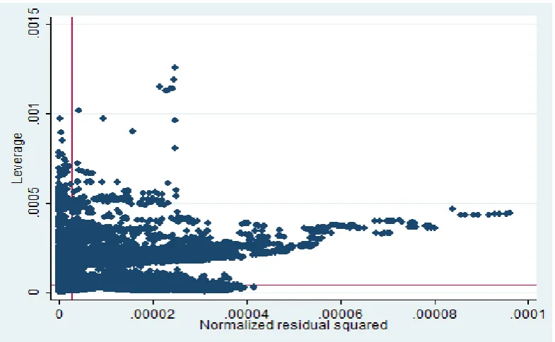
One of the significant challenges of testing gravity test is the difficulty to consider the influence of heteroskedasticity and non-stationarity of time series data on the numerical evaluation of the model. A sample of fitted residuals from the non-robust regression analysis is as follows.
Figure 1: Normalized regression residuals for exploring the behaviour of the model
The distribution of the residuals does not conform to the underlying OLS regression assumption, and it points to a possibility of heteroskedasticity. In this case, conducting a robust
regression leads to the inclusion of population parameters that were excluded from Table 5. The model parameters obtained from the robust regression model are presented as follows.
Table 6: Robust Regression Results
FTA Coef. Std. Err. t P>t
CONT .1773257 .0036173 49.02 0.000
COML .0363915 .0012345 29.48 0.000
DIST -.2122959 .0010041 -211.43 0.000
oPOP -.0292915 .0005437 -53.88 0.000
dPOP -.0292915 .0005437 -53.88 0.000
oGDP .0319653 .0005275 60.59 0.000
dGDP .0319653 .0005275 60.59 0.000
poGDP -2.02e-07 4.29e-08 -4.71 0.000
pdGDP -2.02e-07 4.29e-08 -4.71 0.000
COL .014804 .0040079 3.69 0.000
COMC .0157057 .0035405 4.44 0.000
oEC .0000321 4.46e-06 7.20 0.000
dEC .0000321 4.46e-06 7.20 0.000
oEP -.0055015 .0001578 -34.86 0.000
dEP -.0055015 .0001578 -34.86 0.000
oET .0000728 9.59e-06 7.59 0.000
dET .0000728 9.59e-06 7.59 0.000
Constant .5677447 .0187874 30.22 0.000
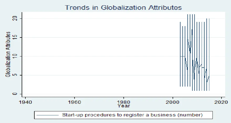
As per Table 6, population and per capita GDP have an inverse relationship with bilateral trade flows, and the finding is in line with what other researchers have discussed. Of interest is the influence of entry cost, entry protocols, and entry time on bilateral
trade flows. As illustrated in the time series plot of these variables, the data on globalization variables are recent through the attributes exhibit a downward trend towards 2015.
Figure 2: The Cost of Entry relative to trading partners.
Figure 2 and Figure 3 illustrates that the cost of starting up a business and the number of procedures required are declining and from the results of the study it was conceived that these trends would improve bilateral trend between pairs of trading countries.
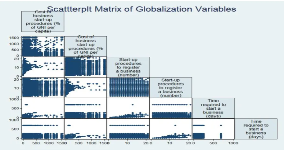
It is prudent to consider the relationship between the cost of entry, number of procedures and the required time so that an efficiency index can be developed to represent globalization in the gravity model. The scatter plot in Figure 4 demonstrates the close relationship between the three attributes.
Figure 4: A Scatterplot Matrix Suggesting the Relationship between the Globalization attributes
Given the obscurity of the dataset, transparent relationships cannot be deduced from the graph, even though cost and start-up procedures appear to develop a linear relationship, just the time required and the number of start-up procedures.
Conclusion
The objective of this research was to establish the influence of globalization variables on the gravity model and its implications on international trade. The model has resulted that addition entry cost, entry procedure, and then the time required to the conventional gravity model has hinted to an increase in the proportion of variations in bilateral trade flows. The model leading to the general hypothesis that globalization is reducing the cost of entry, and total time required to set up. While minimizing bureaucracy associated with registering businesses and launching operations.
The resultant model is as follows:
( ) ( ) ( )
( ) ( )
( ) ( ) ( )
( ) ( ) ( )
( ) ( ) ( )
( ) ( ) ( )
( )
Future studies should consider exploring further the contribution of globalization on bilateral trade flows. Preferably, the analysis should use structural equation modelling (SEM) with trade flow, gravity, and globalization latent variables.
The trade flow latent variable should contain information on export, import, free trade agreements, preferential trade agreements, and union memberships. Such an approach will aid in identifying globalization factors that mediate the interaction between global variables and bilateral trade responses.
Data Availability
The data used in the study were retrieved from different resources the CEPII, www.cepii.fr, the World Bank, www.worldbank.org, and the world factbook,
https://www.cia.gov/library/publications/the-world-factbook/
Conflicts of Interest
I declare that there is no conflict of interest regarding the publication of this paper.
Funding Statement
This research is self-funded by the researcher.
Acknowledgments
The researcher would like to thank Mrs. Reham Omar Al Momany
for her great support and constructive comments.
References
[1] Bergstrand, J. H. (1985). The gravity equation in international trade: some microeconomic foundations and empirical evidence. The Review of Economics and Statistics, 67(3) 474–481.
[2] Blomberg, S. B., & Rosendorff, B. P. (2009). A gravity model of globalization, democracy and transnational terrorism. Creat Homeland Security Center, Claremont, CA 91711, 1-37.
excess zeros and zero-inflated estimation. Spatial Economic Analysis, 4(2), 167–190.
[4] Chaney, T. (2008). Distorted gravity: the intensive and extensive margins of international trade. American Economic Review, 98(4), 1707–1721.
[5] Chaney, T. (2018). The gravity equation in international trade: An explanation. Journal of Political Economy, 126(1), 150–177.
[6] De Benedictis, L., & Taglioni, D. (2011). The gravity model in international trade. The trade impact of European Union preferential policies (pp. 55–89). Springer.
[7] Dias, D. (2011). Gravity and Globalization.
[8] Egger, P. (2002). An econometric view on the estimation of gravity models and the calculation of trade potentials. World Economy, 25(2), 297–312.
[9] Egger, P., & Pfaffermayr, M. (2003). The proper panel econometric specification of the gravity equation: A three-way model with bilateral interaction effects.Empirical Economics, 28(3), 571–580. https://doi.org/10.1007/s001810200146
[10] Feal-Zubimendi, S., Rosas Garc\‟\ia, J. N., Hernaiz, D., & Bastos, F. (2018). Trade Potential in Southern Cone Countries.
[11] Gómez-Herrera, E. (2013). Comparing alternative methods to estimate gravity models of bilateral trade. Empirical Economics, 44(3), 1087–1111.
[12] Grünfeld, L. A., & Moxnes, A. (2003). The intangible globalization: Explaining the patterns of international trade in services.
[13] Head, K., Mayer, T., & Ries, J. (2010). The erosion of colonial trade linkages after independence. Journal of International Economics, 81(1), 1–14.
[14] Kareem, F. O., & others. (2013). Modelling and estimation of gravity equation in the presence of zero trade: A validation of hypotheses using Africa's trade data. In a presentation at the 140th EAAE Seminar, “Theories and Empirical Applications on Policy and Governance of Agri-food Value Chains,” Perugia, Italy (pp. 13–15).
[15] Lewer, J. J., & den Berg, H. (2008). A gravity model of immigration. Economics Letters, 99(1), 164–167. [16] Linders, G.-J., & De Groot, H. (2006). Estimation of the
gravity equation in the presence of zero flows.
[17] Liu, Y., & Luo, R. (2004). Impact of Globalization on International Trade between ASEAN-5 and China: Opportunities and Challenges. Global Economy Journal, 4, 6. https://doi.org/10.2202/1524-5861.1005
[18] Marinov, E., & others. (2014). The direction of international trade of African regional economic communities. In 14th International Academic Conference.
[19] Marti‟nez-Zarzoso, I., & Nowak-Lehmann, F. (2003). Augmented Gravity Model: An Empirical Application to Mercosur-European Union Trade Flows. Journal of Applied Economics, 6(2).
[20] Miron, D., Miclaus, P., & Vamvu, D. (2013). Estimating the Effect of Common Currencies on Trade: Blooming or Withering Roses? Procedia Economics and Finance, 6(13), 595–603. https://doi.org/10.1016/S2212-5671(13)00177-9
[21] Rose, A. K., & Spiegel, M. M. (2004). A gravity model of sovereign lending: trade, default, and credit. IMF Staff Papers, 51(1), 50–63.
[22] Samimi, P., & Jenatabadi, H. S. (2014). Globalization and economic growth: Empirical evidence on the role of complementarities. PloS One, 9(4), e87824.
[23] Savrul, M., & Insecara, A. (2015). The Effect of Globalization on International Trade: The Black Sea Economic Cooperation Case. In International Conference On Eurasian.
[24] Smarzynska, B. K. (2001). Does relative location matter for bilateral trade flows? An extension of the gravity model. Journal of Economic Integration, 379–398. [25] Vioricã, E.-D. (2012). Econometric Estimation of a