Scalable Computing: Practice and Experience
Volume 18, Number 1, pp. 67–89. http://www.scpe.org
ISSN 1895-1767 c
⃝2017 SCPE
PVL: PARALLELIZATION AND VECTORIZATION OF AFFINE PERFECTLY NESTED-LOOPS CONSIDERING DATA LOCALITY ON SHORT-VECTOR MULTICORE
PROCESSORS USING INTRINSIC VECTORIZATION
YOUSEF SEYFARI, SHAHRIAR LOTFI, AND JABER KARIMPOUR∗
Abstract. There is an urgent need for high-performance computations. Cores and Single Instruction Multiple Data (SIMD) units are important resources of modern architectures to speed up the execution of programs. Also, the importance of the data locality cannot be neglected in computations. Using cores, SIMD units, and data locality simultaneously is critical to gain peak performance of the architecture. But, there are a few research efforts trying to consider these three resources at the same time. There is a challenge in choosing loops which could be whether run on SIMD units or cores for vectorization and parallelization, respectively. This paper proposes an approach, named PVL, for parallelization and vectorization of nested loops considering data locality based on the polyhedral model on short-vector multicore processors. More precisely, PVL, tries to satisfy dependences in the middle levels of nested loop (the levels between outermost and innermost levels) while trying to move dependence-free loops to the outermost and innermost position in order to parallelize and vectorize them, respectively. The experimental results show that the proposed approach, PVL, is significantly effective compared to the other approaches.
Key words: short-vector multicore processors, parallelization, vectorization, perfectly nested-loops
AMS subject classifications. 65Y05
1. Introduction.
1.1. Motivation. Since the computers have become publicly available, the demand for more increasingly speed has not vanished. However, it becomes more difficult to speed up the processors by increasing the frequency. Two major problems with speeding up the processors are overheating and power consumption [1, 2]. One of the proposed solutions to these barriers is multicore architecture. Nowadays, there is a growing trend in processor industry towards multicore processors. This trend has involved two different areas: (1) ordinary users and (2) supercomputers. Presently, typical users can get better response time in CPU-intensive applications due to improved multitasking with the help of multicore processors. The appearance of multicore architecture also has brought the supercomputing area into a new era. In fact, multicore processors have already been widely used in parallel computing. Lei et al. [2], in 2007 reported that more than 20% of supercomputers processors are multicore processors, but in the last report of Top500 supercomputer list published in November 2016, there is no supercomputer with single core processor. In other words, 100% of processors of supercomputers are multicore processors [3]. These facts accentuate the importance of effective use of multiple cores.
Besides executing different instructions on multiple processing units simultaneously, namely parallelism, an alternative approach has been proposed which employs certain instructions called vector instructions [4]. Vector instructions would initiate an element-wise operation on two vector quantities in vector registers which could be loaded from memory in a single operation; these machines are called vector machines [5]. Since the late 90’s, specialized processing units called Single Instruction Multiple Data (SIMD) extensions have been included in the instruction set architecture (ISA) of processors to exploit a similar kind of data parallelism as vector machines [6]. However, since the width of these vector instructions is relatively small, they are also called short-vectors [7]. But due to the growing demand for speed, the width of vector-SIMD instruction sets is constantly increasing (for example, 128 bits in SSE [8], 256 bits in AVX [9] and 512 bits in LRBni [10]). According to Cebrian et al. [11], in addition to the performance, vectorizing using short-vectors has also a great impact on energy efficiency. These highlights the significance of the effective use of SIMD vectors. The problem gets more complicated when both parallelization and vectorization are considered together.
1.2. The problem. Today, computations from complex scientific computations such as signal and image processing demand high-performance computing to be solved faster. These problems are characterized by long running computations with spending most of their running time in nested loops. Due to the long consumed
∗Department of Computer Science, Faculty of Mathematical Sciences, University of Tabriz, Tabriz, Iran (seyfari @tabrizu.ac.ir, shahriar [email protected], [email protected]).
time in the loops, they are privileged candidates for parallel execution on both kinds of mentioned process-ing resources: (1) multiple cores and (2) vector-SIMD. In order to fulfill the computprocess-ing needs of scientific computations, it is essential to use both multiple cores and vector-SIMD effectively.
Listing 1
The general form of the perfectly nested loops
for(i1=L1;i1<=U1;i1+ =T1){ for(i2=L2;i2<=U2; i2+ =T2){
...
for(in=Ln;in <=Un; in+ =Tn){
S1: A[f1(i1, i2, ..., in), f2(i1, i2, ..., in), ..., fm(i1, i2, ..., in)] =... S2: ...=A[g1(i1, i2, ..., in), g2(i1, i2, ..., in), ..., gm(i1, i2, ..., in)]
} ... } }
Listing 1, illustrates the general form of an n-dimensional perfectly nested loop with loop indicesi1, i2, ..., in from the outermost to the innermost loop respectively. Each loop with index k, in the loop nest has a lower bound Lk, an upper bound Uk and a loop step of Tk. The body of the innermost loop in perfect loop nest contains some statements that usually have some arithmetic calculation on arrays. The subscript of arrays is an affine function (f, g) of loop indices [5].
In this paper, we consider the problem of parallelization and vectorization of perfectly nested loops with dependences on modern architecture with cores and short-SIMD. With respect to the different sources for parallel execution including multiple cores and vector-SIMD, there are two kinds of loops: (a) loops that do not carry any dependences, that is, parallel loops which can be executed without any problem in different cores, (b) loops that do carry dependences, that is, this loops have to be executed serially. Among two different approaches for parallel execution namely cores and vector-SIMD, later one requires more constraints than cores. In addition to not having dependence carried by the loop, in order to vectorize them effectively without any overhead it is better the data to be contiguous in the memory. So, a few factors must be considered to run a nested loop on modern architectures with two different sources for parallel execution including multiple cores and vector-SIMD:
1. Multiple cores are used for coarse-grained parallelism, so having parallel loop at outermost level of nested loop is required to get better performance. In case the parallel loop is not in the outermost position, we have to move candidate parallel loop to the outermost level if possible;
2. In order to use vector-SIMD to execute different iterations of a loop in parallel, it is better the data accessed by that loop be contiguous in the memory; in arrays, if it is row-major in memory, the contiguous data is the data in the last dimension of the array, that is, rightmost subscript in the arrays. Else, the contiguous data is the ones in the first dimension of the array, that is, leftmost subscript in the arrays (so contiguous data can be packed in vector registers and can be operated on by vector instructions);
3. Loops have to be dependence-free since our focus is on loops for executing in multiple cores or vector-SIMD.
perform a loop strip-mining transformation before using ILP. For further description see Sec. 3. After having a parallel loop at the outermost position and vector loop at the innermost position, we generate intrinsic vector codes for the innermost vector loop and its statements.
1.3. Contributions. The main contributions of this paper are as follows:
• We propose a unified approach for parallelizing and vectorizing perfectly nested loops simultaneously with respect to the data locality.
• We use ILP with an objective function to get a proper transformation in order to parallelize, vectorize, and improve data locality of the given nested loop at the same time.
• To vectorize innermost vectorizable loop, we propose to generate intrinsic vector code from binary expression tree of the statements inside the loop body.
1.4. Paper outline. The remaining sections of this paper are organized as follows: after introduction, Sec. 2 includes mathematical basic concepts and a brief review of some related works. Section 3 includes the proposed approach. Section 4 includes evaluation and experimental results. Finally, Sec. 5 is dedicated to the conclusions.
2. Polyhedral Model and Related Work. In this section, after introducing required concepts for the polyhedral model, related works are presented.
2.1. Polyhedral Model. An important part of parallelizing/optimizing compilers is the transformation of programs. In this paper, by program transformation we mean loop-restructuring transformation since we focus on the loops. In order to apply transformations on loops easily and effectively, the abstract representation model of the loops is required. Polyhedral model is a powerful and flexible mathematical framework used for representing programs. It is based on a linear algebraic representation of programs [1, 13]. However, not all loops can be represented by polyhedral model except static control parts (SCoPs) [13, 14]. A SCoP is defined as a maximal set of consecutive statements, where loop bounds and conditionals are affine functions of the surrounding loop indices and parameters. The majority of scientific and engineering calculation kernels belongs to this class or can be re-expressed as SCoP [12].
The polyhedral model has four basic components to represent loops: (1) the iteration domain, (2) the access function, (3) dependence polyhedral and (4) the transformation.
The iteration domain is used to represent the dynamic instances of each statement in the loop body using a system of affine inequalities. The system of affine inequalities is derived from loop bounds enclosing the statement. Each derived inequality has to be expressed in the Ax+b≥0 form and iteration domain of a statement is expressed in theD={−→x|−→x ∈Zn, A−→x+−→b ≥−→0}form where−→x = (x1, x2, ..., xn)T is the iteration vector representing a loop nest with depth nandxk is thekth loop index in the loop nest. The possible value for each loop index is an integer, so each entry of the iteration vector is the member of Z.
For instance, in Listing 2 , the iteration vector is −→x = (i, j)T and the iteration domain of statement S is DS ={(i, j)|0≤i≤N,0≤j≤M}and its matrix form is as (2.1).
Listing 2
The convolution kernel
for(i= 0; i <=N;i+ +){ for(j= 0; j <=M; j+ +){ S: y[i] =y[i] +b[j]×x[i+j]
} }
DS =
1 0
−1 0
0 1
0 −1
(
i j
)
+
0 N 0 M
≥−→0 (2.1)
There is an instance of memory reference for each point in the iteration domain of some statement likeS. Each instance of memory reference accesses a cell of array A that is shown by access functionFS
A(−→xS).
Thedependence polyhedralis used to represent the data dependences in the loop nest. There is a data dependence between statementsS1andS2if and only if both statements refer to the same memory location (that is the same cell of array) and at least one of them is a write, the statement that executes first is the source and the statement that executes later is the sink. The dependence polyhedral is essential in parallelizing/optimizing loops since they determine the transformations that preserve the meaning of the program and it models the dependences in the program using a set of equalities and inequalities. For example dependence polyhedral for Listing 2 isDS,S={(i, j, i′, j′)|0≤i≤N,0≤j≤M,0≤i′ ≤N,0≤j′≤M, i=i′}and its matrix form is as (2.2).
DS,S =
1 0 1 0
1 0 0 0
−1 0 0 0
0 1 0 0
0 −1 0 0
0 0 1 0
0 0 −1 0
0 0 0 1
0 0 0 −1
i j i′ j′ + 0 0 N 0 M 0 N 0 M = 0
≥−→0 (2.2)
The transformations in the polyhedral model are used to change the iteration order of original loop nests. A program transformation in the polyhedral model is represented by a function that determines the logical order of statement instances based on surrounding loop indices of the corresponding statement, called scheduling function [14, 15].
Loop transformations have been applied to improve instruction scheduling, register use and cache locality and also to expose parallelism [16]. There are a lot of transformations such as loop reversal, loop interchange, loop distribution, strip-mining and so on. Because some loop transformations only reorder the iterations of a loop nest these are categorized into one group named Iteration-reordering transformations such as loop interchange and strip-mining; in addition to iteration-reordering some other loop transformations also reorder statements, statement instances and/or the operations within a statement such as loop distribution [16].
Some loop transformations can be represented using a scheduling matrix Θ. For example in loop iterators
(
i j
)
of a 2-d loop nest, the loop interchange transformation can be shown by Θ
( i j ) = [ 0 1 1 0 ] ( i j ) and loop
reversal transformation can be represented by Θ
( i j ) = [ −1 0 0 1 ] ( i j )
. Because the final aim of transformation
stage in this work is to expose hidden parallelism as a coarse-grained parallelization as well as a fine-grain vectorization, the most useful transformations are the strip-mining and the loop interchange; however loop strip-mining cannot be represented as a matrix.
Listing 3
The strip-mined convolution kernel
k=ceil(N/P);
for(I= 0;I <=N;I+ =k){
for(i=I;i <=min(I+k−1, N);i+ +){ for(j = 0;j <=M;j+ +){
S: y[i] =y[i] +b[j]×x[i+j]; }
} }
2.2. Legality of Transformations in Polyhedral Model. In order to parallelize/vectorize loops during the process of loop transformation, the semantic of the program should not change, that is, transformed program should generate the same outputs with the same order as the original program; otherwise, the transformation is not legal. In order to have a legal transformation, it must satisfy (preserve) dependences in the program. There are four kinds of data dependences: input-dependence, true-dependence, anti-dependence and output-dependence [5]. However, violating the input-output-dependence does not affect the meaning of a program.
Given data dependenceebetween statementsSandT, dependenceeis said to be satisfied if for all pairs of dependent instances⟨−→XS,
− →
XT⟩the source is executed before the sink. In other words, the schedule of the source instance is smaller than the schedule of the sink instance, i.e., if Θ represents the scheduling of statements, for all pairs of dependent instances: Θ(−→XS)<Θ(
− →
XT) and for statements the schedule of source statement,S, is smaller than the schedule of sink statement T: Θ(S)<Θ(T). Applying a transformation Θ on a program is legal if and only if (2.3) holds.
∀e∈E∀⟨−→XS, − →
XT⟩ ∈DS,TΘT( − →
XT)−ΘS( − →
XS)≥0 (2.3)
where DS,T is dependence polyhedral of statements S andT.
2.3. Related Work. Parallelization and vectorization are two important techniques to execute different iterations of loops simultaneously. However, most of the previous works have considered only one of them; while in order to get better performance, parallelization and vectorization have to be considered together since modern processors support both types of parallelization. Generally, works in loop optimization can be categorized into three different fields: improving data locality with loop transformations, loop tiling, and data transformations.
Data localityis a very important factor in improving the performance of the programs and especially loops [18, 19]. One of the important methods to deal with data locality is loop transformation such as loop fusion and loop distribution and others. Naci in 2007 [20] tried to improve data locality of loops with loop transformations. Ozturk in 2011 [21] presented a method based on constraint satisfaction problem (CSP) to handle data locality and parallelizing of loop nests. Parsa et al. [22] proposed a method to expose coarse-grain parallelism by reusing data to execute loops on multicore processors. They tried to find a scheduling function for nested loops using a polyhedral model that makes iterations of outer loops independent and consequently parallel. To find such a transformation (scheduling function), they tried to satisfy dependences in inner loops. Doing so, the reuse distance of the data is reduced. It is notable to mention that making outer loops dependence-free and moving dependencies to inner loops has achieved just by the only main idea: to satisfy dependencies at inner loops. To use vector-SIMD units of processors, the innermost loops have to be dependence-free, that is, either the innermost loop does not carry any dependences or if it carries some dependences, then another candidate dependence-free loop should be moved to the innermost position if it is legal. However with their idea, they make the innermost loops to carry dependencies and as a result, they miss vectorization chance. Not only they have not considered the important technique of vectorization, but also their idea inhibits any next vectorization.
in iteration space as a chromosome in GA. This method has some advantages including having no restrictions on loop dimensions and also after tiling, nested-loops can be executed in parallel. However, vectorization is not considered in this work. Krishnamoorthy et al. in 2007 [26] presented a method to tile loops for eliminating pipelined start and drained finish of the tiles. With this method in addition to improving data locality and gaining coarse-grained parallelization, they addressed the problem of unbalanced execution of tiles in multi-core systems. Bondhugula et al. in 2008 [27] proposed an iteration space tiling method based on polyhedral to execute on multicore processors. In this work, they presented a cost model to obtain parallelization and data locality at the same time. The aims of this tiling are minimization of communications and increasing data reuse in each processor. The advantage of this work is that it can be used on loops with any dimensions and the disadvantages of this work are the delays of pipelined start-up and drain of tiles and also vectorization has not been considered in this work. Bandishti et al. in 2012 [28] presented a new tiling method. This method was replaced traditional parallelopiped tiling in Pluto compiler.
Data layout transformation is another technique that has been using for preparing loops both to enable vectorization and also for improving data locality in the new architectures [29, 30]. Lu in 2009 [31] presented a data layout transformation method for optimizing data locality in multi-processor architecture of Non-Uniform Cache Architecture (NUMA). Jang et al. in 2010 [32] presented a mathematical model for acquiring access patterns of data and then computing the most proper data transformation in order to vectorize loops.
A number of the works have addressed the problem of parallelization and vectorization of the programs, however, they either focused on a very special kind of CPU like iPSC-VX or they tried to parallelize or vectorize a special programs only. These works are reviewed in the following section.
Krechel et al. [33] investigated parallelization and vectorization strategies for the solution of large tridi-agonal linear systems on MIMID computers which have vector processors. In their experiments, they try to minimize communication on message-based computing systems and maximize the parallelism. In particular, they presented a distribution of large tridiagonal systems across different processes on iPSC2-VX architecture. Aykanat et al. [34] implemented Conjugate Gradient algorithm for exploiting both parallelization and vectoriza-tion on iPSC-VX/d2 architectures with 2-dimensional hypercube and used it to solve large sparse linear systems of equation. They achieve efficient parallelization by reducing communications and overlapping computations on the vector processor with internode communication. Crawford et al. [35] proposed a vectorization and parallelization approach for the application of the adiabatically-adjusting principal axes hyperspherical(APH) Hamiltonian used in time-dependent quantum reactive scattering calculations. They separate Hamiltonians for APH coordinates into its constituent parts and vectorize these to speedup computations required in matrix multiplications and then parallelize.
3. The Proposed Approach. In this section, we propose an approach for parallelizing and vectorizing perfectly nested loops with dependences on modern architecture with cores and short-SIMD.
There are two different cases in the original loop nest that have been dealt with in the proposed method. In the first case, the original loop nest has more than one dependence-free loop one of whose has contiguous data in the memory and in the second case the original loop nest has just one dependence-free loop whose data is contiguous in the memory. In the first case, employing loop strip-mining is not required and it is sufficient to use loop interchange transformation to move parallel/vector loop to proper positions.
Listing 4
The summation kernel, C=A+B
for(j= 0; j <=N;j+ +){ for(i= 0;i <=M;i+ +){ S: C[i, j] =A[i, j] +B[i, j]
} }
Listing 5
The loop interchanged summation kernel, C=A+B
for(i= 0; i <=M;i+ +){ for(j= 0; j <=N;j+ +){ S: C[i, j] =A[i, j] +B[i, j]
} }
However, in the second case where there is just one dependence free loop, the usage of loop strip-mining is unavoidable to have both parallel and vector loops. For example in order to parallelize and vectorize the loop nest in Listing 2, since there is just one dependence-free loop, using loop strip mine with step sizesk on loopi results two dependence-free loopsI, and i(Listing 3) that loopican be vectorized. In order to vectorize loop i, it has to be moved to the innermost position by a proper transformation.
In addition to the cores and short-vectors, the data locality has a significant effect on the execution time of the programs. So, besides parallelization and vectorization, we try to find a transformation that has improved data locality according to the storage layout of the array whether it is row-major or column-major. In this order, we have used an ILP-based method to obtain proper transformation.
3.1. ILP formulation. In this section, a new ILP based method, PVL, is proposed to obtain proper loop interchange transformation that enables coarse-grained parallelism and fine-grained vectorization. Generally, when formulating a problem in ILP, there is an objective function we want to maximize/minimize and some constraints with respect to which the objective function has to be satisfied.
It has been shown [5] that cores are best suited to coarse-grained computations in new short-vector multicore architectures and the computations of outer loops are more coarse-grained than inner loops in loop nests. Hence, in the loop nest, it is better to move the parallel loop to the outermost position- that is, the outer the loop, the more coarse-grained the computations. On the other hand, parallelism is fine-grained in the short-vectors. Loops with contiguous data which are in the innermost position can be executed in short-vectors.
3.1.1. Formulating Objective Function. Loop interchange transformation is a square matrix n×n whichnis the dimension of the original loop nest and it can be represented as a matrix in which entries belong to {0,1}, such that there is just a single one in each row as well as each column; the original scheduling of strip-mined convolution is as (3.1) where the iteration order of strip-mined convolution would not change by this transformation.
Θ =
1 0 0
0 1 0
0 0 1
(3.1)
Having just a single one in each row in loop interchange transformation, it can be formulated as a constraint in ILP (3.2).
|dimensions|
∑
i=1
ci= 1 (3.2)
To obtain proper transformation using proposed ILP based method, transformation Θ will be produced row by row. For a three-dimensional loop, each row of Θ in general, is denoted by (ci, cj, ck) such that each entry has a value. Hence, in order to get proper values of ci, cj, and ck, the objective function of ILP has to be a function of row’s entries such that it satisfies parallelization, vectorization, and data locality in the transformed loop nest. In order to create the objective function, it is required to notice the behavior of the transformation matrix. For a three-dimensional loop nest, given loop interchange transformation Θ is composed of three rows:
Θ =
c1i c1j c1k c2i c2j c2k c3i c3j c3k
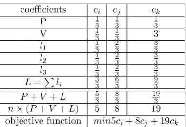
Table 3.1
Creating the objective function for a sample 3-dimensional loop
coefficients ci cj ck
P 1
3 1 3
1 3
V 1
3 1
3 3
l1 1
3 2 3
3 3
l2 1
3 2 3
3 3
l3 1
3 2 3
3 3
L=∑l
i 33
6 3
9 3
P+V +L 5
3 8 3
19 3
n×(P+V +L) 5 8 19
objective function min5ci+ 8cj+ 19ck
In this transformation, each row is dedicated to a loop through loop nest, and each column is representing the position of the corresponding loop (row) in the loop nest, that is, if the first row of Θ is (0,1,0), it denotes that the position of the first loop in transformed loop nest would be the second position. As explained so far, with respect to the final aim of parallelization and vectorization at the same time in the loop nest, it is required that first row and last row of the transformation Θ show the parallel and the vector loops, respectively. However, since in the proposed method transformation Θ is obtained row by row from the outermost row to the innermost row, it is clear that the parallel loop has to be selected at first and the vector loop has to be selected at last. In the following transformation Θ, the row denoting parallel loop is highlighted as green (box with dashed line) and the row denoting vector loop is highlighted as blue (box with dotted line).
With these explanations, in the objective function of the proposed method the priority of the parallel loop is selected as the highest and the priority of vector loop is selected as the lowest. In the other hand, loop nests may have some loops neither parallelizable nor vectorizable; these loops are the loops with dependence and transformation Θ is legal if it satisfies all dependences in the loop nest. Since the first and last rows represent parallel and vector loops respectively, so dependences have to be satisfied in the middle rows highlighted as red (box with solid line) in the transformation, so the priority of loops with dependence is mid. By middle rows we mean the rows of the transformation Θ that are between the first and the last rows. Because the formulated ILP problem in Sec. 3.1.1 is a minimization problem, the loops with the highest priority (parallel loops) have smallest coefficients and similarly the loops with the lowest priority (vector loops) have the highest coefficient. Hence, the objective function of sample three-dimensional loop nest in Listing 6 is created according to the Table 3.1.
Listing 6
Sample 3d-loop
for(k= 0;k <= 100;k+ +){ for(j= 0; j <= 100;j+ +){
for(i= 0;i <= 100;i+ +){ S: A[i, j, k] =A[i, j, k] +B[i, j, k];
} } }
vector which are described as follows:
Data localityin this paper means whether the arrays are stored in the memory as row-major or column-major. There is a row (i.e. l1, l2, ...) in the table for each reference. The final locality, L, is defined as L=∑li. Values of eachl
iin the table is computed as follows: if arrays are stored as row-major in the memory, li,j = dimensionj loop, where lij is the value in column cj of row li. If arrays are stored as column-major in
the memory, li,j = dimensionloop−j +1
dimensionloop . In this example, it is assumed that the arrays are stored as row-major.
So, the first row of data locality, l1, is for the first reference in the statement within loop nest i.e. A[i, j, k] (left-hand-side). The values of this row are 1
3, 2 3, and
3
3. In this example dimensionloop = 3 and because the loop indexi is the first subscript in the reference, so its value is 13, and so on.
Parallelparameter denotes the loops which its iterations can be executed in parallel. Values of this row in the table belong to{n,1
n}wherenis the number of dimensions. The presence ofnmeans that the iterations of the corresponding loop can not be executed in parallel, and the presence of 1
n means that the iterations of the corresponding loop can be executed in parallel. In Listing 6, iterations of all loops can be executed in parallel, so the values of all entries of this row are 1
n.
Vector parameter denotes the loops with contiguous data which do not carry any dependence. Values of this row in the table belong to {n, 1
n}, where n is the number of dimensions. The presence of n means that the corresponding loop can be vectorized and the presence of 1
n means that the corresponding loop is not vectorizable. In this example, the loop with indexkcan be vectorized. So in the table, vector parameter of this loop is 1
3 (heren= 3) and other loops are 3.
Finally, the parameters of Table 3.1 is used as n×(P+V +L) to obtain the objective function, wheren is the number of dimensions andP,V, andLare parallel, vector and locality parameters, respectively.
3.1.2. Automatically Getting Objective Function from Data Dependences. In order to automat-ically obtain objective function from data dependences, Algorithm 1 is proposed. As explained in the Sec. 3.1.1, the loops that could be executed in parallel will be run in the cores, because the formulated ILP problem in the previous section is minimization, in step 1 the algorithm gives the lowest coefficient 1
n for all of them, denoting that one of these loops should be scheduled first. The loops that could be vectorized will be run in the short-vectors within each core, so the algorithm gives the highest value nfor them, denoting that one of these loops should be scheduled last, where nis the number of dimensions. The arrays storage layout is used in the algorithm to have better data locality. In step 2, the objective function is get byP+V +Land since all terms of objective function have denominator n, the final objective function is get byn×(P +V +L) which omits denominators.
3.2. Formulating Constraints. In the following subsections, constraints of the problem are formulated for ILP
3.2.1. Legality of Transformation. One of the benefits of using polyhedral model is that legality of the obtaining transformation can be verified with a built-in set of constraints obtained from Rel. 2.3 [36]. To create the set of semantic-preserving constraints using Rel. 2.3, for each dependence that is for every dependent statements S and T, the obtained legality constraint from (2.3) is (3.3) and in the case of non-uniform dependences, the obtained nonlinear constraint is converted to linear using Farkas lemma [1, 22, 37].
ΘT(−→XT)−ΘS( − →
XS)≥0 (3.3)
3.2.2. Linearly independence rows. After obtaining the transformation Θ, it is required to be applied on the original polyhedron A−→x +−→b ≥−→0 defining the original loop nest. Scattering function leading to the target index −→y = Θ−→x , the polyhedron of the transformed loop nest is defined by (3.4) [12, 15].
(AΘ−1)−→y +−→b ≥−→0 (3.4)
Algorithm 1Automatically obtain objective function for ILP
Input: Data Dependence Matrix
Output: Objective Function
Step1: //for each loop in the loop nest fill the parallel and vector parameters of //Objective Table (OT), Table 3.1 in the paper
n=number of dimensions
forloop index i=1 tonumber of dimensionsdo
//parallel
if (loopLi carries any dependences) then OT[′parallel′, i] =n;
else
OT[′parallel′, i] = 1 n;
end if
//vector
if (loopLi does not carry any dependences AND Loop index ofLi has contiguous data in the memory)
then
OT[′vector′, i] =n;
else
OT[′vector′, i] = 1 n;
end if end for
//locality
foreach reference within loop nest do
forloop index i=1tonumber of dimensionsdo
if arrays are stored as row-major in the memorythen
OT[′locality′, i]+ = j
dimensionloop if this loop index, i, is the jth subscript of the array
else
OT[′locality′, i]+ = dimensiondata−j+1
dimensionloop if this loop index, i, is the jth subscript of the array
end if end for end for
Step 2:
forloop index i=1 tonumber of dimensionsdo
foreach of the parameters (parallel, vector, and locality)do
coefficient of the loopLi in the objective function,coef f icienti= n×(OT[′parallel′, i] +OT[′vector′, i] +OT[′locality′, i]);
end for end for
in order to Θ be invertible, its rows have to be linearly independent. To this order, in the process of obtaining Θ, after obtaining each row a new constraint is added to the set of the constraints of ILP formulation of new row by (3.5) that ensures the solutions are linearly independent [1, 38, 39].
Θ⊥S =I−ΘTS(ΘSΘTS)− 1
ΘS (3.5)
∀i,Θi⊥
S θS∗ ≥0∧
∑
i Θi⊥
In (3.5) and (3.6), ΘS is the obtained transformation for statementSso far, ΘT
S is the transposition of ΘS, I is the identity matrix andθ∗
S is the next row to be found for statementS.
3.3. The Proposed Algorithm. Algorithm 2 is proposed to obtain the transformation used to parallelize and vectorize nested loops simultaneously. In the first step, if there is not enough dependence-free loop for both parallelization and vectorization, loop strip-mining transformation will be applied to have enough dependence-free loops for both parallelization and vectorization. The constraints of ILP will be built in the steps 2 and 3. In step 2, the loop interchange constraint will be built e.g. for a three-dimensional loop the loop interchange constraint is as Rel. 3.2. In step 3, legality constraints will be built according to the data dependences of the given loop nest using Rel. 3.3. The transformation matrix Θ (T in the algorithm) will be found in step 4. Step 4 is used in this algorithm to obtain objective function for each row in the transformation matrix Θ. In this step, after finding each row of the transformation matrix, the linearly independence constraint is added to the constraints set using Rels. 3.5 and 3.6.
Algorithm 2PVL algorithm
Input: Data Dependence Graph (DDG), Dependence polyhedron (DS,T) for each edge in DDG
Output: Transformation matrix T
Step 1:
if (there is not enough dependence-free loop)then
Apply loop strip-mining
end if
Step 2: //build loop interchange constraint
Add ∑
i=|dimensions|
ci = 1 to constraints-set
Step 3: //build legality constraints
for(each dependence e in DDG)do
Build legality constraintsLCeand add to constraints-set
if (e is nonuniform)then
Apply Farkas lemma and get linearized constraints
end if end for
Step 4: //obtain transformation matrix T using ILP formulation
for (each dimensions of original loop nest)do
//objective function:
obj fun = Get new objective function using Algorithm 1 (input:D) r = ILP-SOLVE(obj fun, constraints-set)
Add row r to T
Eliminate satisfied dependences from D
Add linearly independent constraints to constraint-set
end for
Fig. 3.1.The binary expression tree of y[i] = y[i]+b[j]×x[i+j]
two states are possible. In the first state, the subscript of reference in the statement contains loop index i, such as y[i] in this statement. In this state, the intrinsic vector load will load four contiguous elements y[i], y[i+1], y[i+2] and y[i+3] of array y. In the second state, the subscript of reference in the statement does not contain loop index i, such as b[j] in this statement. In this state, the corresponding register vector will load the same element b[j] four times (b[j], b[j], b[j], and b[j]). For example if the statement of the innermost loop is y[i]=y[i]+b[j]×x[i+j] and the loop index of the innermost loop isi, binary expression tree and corresponding intrinsic vector codes are as Fig. 3.1 and Listing 7, respectively. If the current statement within loop nest requires more vector registers than available vector registers in the underlying architecture, then we split that statement into some sub-statements and store result of each sub-statement in a temporary vector register than gather all temporary vector registers in order to make up the result of that statement.
Listing 7
Intrinsic vector code of Fig. 3.1
m128 y4= mm loadu ps(&y[i]); m128 b4= mm set1 ps(b[j]); m128 x4= mm loadu ps(&x[i+j]);
y4 = mm add ps( mm mul ps(b4, x4), y4); mm storeu ps(&y[i], y4);
3.5. Example. In this section, Algorithm 1 and Algorithm 2 are used step by step in order to obtain a proper transformation for following loop nest, which upper bound of loops, N, is divisible by four:
Listing 8
Example loop nest
for(i= 1; i < N; i+ +){ for(j= 1; j < N; j+ +){
for(k= 0;k < N;k+ +){ for(l= 0;l < N;l+ +){
S: A[i, j, k, l] =A[i−1, j−1, k, l] +B[i−1, j−1, k, l]; }
} } }
The iteration domain polyhedron for statementS within the loop nest is:
DS ={(i, j, k, l)|1≤i≤N−1,1≤j≤N−1,0≤k≤N−1,0≤l≤N−1}
The dependence polyhedron for flow dependence (RAW: read after write) from the write at A[i, j, k, l] to the read at A[i−1, j−1, k, l] for any two iterations,I= (i, j, k, l) andI′= (i′, j′, k′, l′) is:
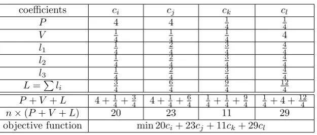
Table 3.2
Creating the objective function for the first row of the transformation matrix for the example loop nest
coefficients ci cj ck cl
P 4 4 1
4 1 4 V 1 4 1 4 1 4 4 l1 1 4 2 4 3 4 4 4 l2 1 4 2 4 3 4 4 4 l3 1 4 2 4 3 4 4 4
L=∑l
i 34
6 4 9 4 12 4
P+V +L 4 +1
4+ 3
4 4 +
1 4+ 6 4 1 4+ 1 4 + 9 4 1 4+ 4 +
12 4
n×(P+V +L) 20 23 11 29
objective function min 20ci+ 23cj+ 11ck+ 29cl
Because this loop nest has two loops with independent iterations, so Step1 of the Algorithm 2 is not required. The loop interchange constraint for this loop nest using Rel. 3.2 is:
ci+cj+ck+cl= 1
and the legality constraints for this dependence using Rel. 3.3 is as follows:
(ci, cj, ck, cl)×(i, j, k, l)T −(ci, cj, ck, cl)×(i′, j′, k′, l′)T ≥0
(ci, cj, ck, cl)×(i, j, k, l)T −(ci, cj, ck, cl)×(i−1, j−1, k, l)T ≥0 ci+cj ≥0
Now the constraints of ILP are determined. The objective function of the ILP is created according to the Table 3.2. In this table, because the loops i and j carry dependence, the corresponding values for these loops in row P (parallel parameter) arenand because the iterations of the loopsk andl are independent the corresponding values for these loops in rowP are 1/n, whichnis number of dimensions (n= 4). The values of rowV (vector parameter) corresponding with loopsiandjare 1/nmeans they are not vectorizable because of the dependence and the value of loop kis 1/n denoting that although iterations of this loop are independent but the data corresponding with this loop in the arrays are not contiguous. Hence, the loopk is not preferred to be vectorized. The value of the looplisn, denotes that this loop is preferred to be vectorized (whichnis the number of dimensions, heren= 4). The locality parameter is the aggregation of thelis, the locality status of each reference within the statement of the loop nest. Since in this example data layout is row-major, for each reference the locality is calculated based on dimensionj
loop, where j denotes that this loop index is jth subscript
in the reference from the left. The final objective function ismin20ci+ 23cj+ 11ck+ 29cl. So, the ILP problem for the first row of the transformation matrix is as follows:
min 20ci+ 23cj+ 11ck+ 29cl s.t. (1)ci+cj+ck+cl= 1;
(2)ci+cj≥0; (3)ci≥0; (4)cj≥0; (5)ck≥0; (6)cl≥0;
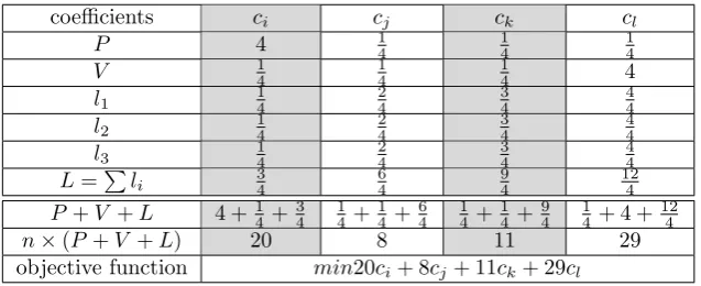
Table 3.3
Creating the objective function for the third row of the transformation matrix for the example loop nest
coefficients ci cj ck cl
P 4 1
4 1 4 1 4 V 1 4 1 4 1 4 4 l1 1 4 2 4 3 4 4 4 l2 1 4 2 4 3 4 4 4 l3 1 4 2 4 3 4 4 4
L=∑l
i 34
6 4 9 4 12 4
P+V +L 4 +1
4+ 3 4 1 4+ 1 4+ 6 4 1 4+ 1 4+ 9 4 1 4+ 4 +
12 4
n×(P+V +L) 20 8 11 29
objective function min20ci+ 8cj+ 11ck+ 29cl
matrix, the linear independence constraint is added to the constraints set according to the Rels. 3.5 and 3.6:
Θ⊥S =
1 0 0 0
0 1 0 0
0 0 0 0
0 0 0 1
hence, the linear independence constraintci+cj+cl≥1 should be added to the constraints set. The ILP formulation for obtaining the second row of the transformation matrix is as follows:
min 20ci+ 23cj+ 11ck+ 29cl s.t. (1)ci+cj+ck+cl= 1;
(2)ci+cj≥0; (3)ci≥0; (4)cj≥0; (5)ck≥0; (6)cl≥0;
(7)ci+cj+cl≥1;
The solution of the above ILP problem gives (1, 0, 0, 0) for the coefficients (ci, cj, ck, cl) of the second row of the transformation matrix. This row of transformation matrix determines the position of the loop i. To obtain the next solution for the third row, linear independence constraintcj+cl≥1 should be added to the constraints set. Because the RAW dependence is carried by this loop, after finding the position of this loop, this dependence will be satisfied and therefore will be removed from the dependence graph and constraints set (ci+cj ≥0). So, the objective function for the next row will change as Table 3.3. The positions of the loops i andkare determined already. Therefore, because of linear independence constraint the values of coefficients corresponding with the loops i and k in the next rows will be zero. Hence, their columns in the Table 3.3 will not have any effects on the solution of the next row. So, we do not change the values of these columns in Table 3.3.
The ILP formulation for obtaining the third row of the transformation matrix is as follows:
min 20ci+ 8cj+ 11ck+ 29cls.t. (1)ci+cj+ck+cl= 1;
(2)ci≥0; (3)cj≥0; (4)ck≥0; (5)cl≥0; (7)cj+cl≥1;
the transformation matrix. This row of transformation matrix determines the position of the loopj. To obtain the next solution for the fourth row, linear independence constraintcl≥1 should be added to the constraints set. Because after finding the third row of the transformation matrix the dependence graph does not change, so the objective function for the next row will not change.
The ILP formulation for obtaining the fourth row of the transformation matrix is as follows:
min 20ci+ 8cj+ 11ck+ 29cls.t. (1)ci+cj+ck+cl= 1;
(2)ci≥0; (3)cj≥0; (4)ck≥0; (5)cl≥0; (7)cl≥1;
The solution of the above ILP problem gives (0, 0, 0, 1) for the coefficients (ci, cj, ck, cl) of the fourth row of the transformation matrix. Therefore, the final transformation matrix is as follows:
Θ =
0 0 1 0
1 0 0 0
0 1 0 0
0 0 0 1
Applying the transformation matrix Θ to the original loop nest moves the loop kto the outermost position as a coarse-grained parallel loop and the loopl to the innermost position as a fine-grained vector loop. Listing 9 shows the resultant final loop nest after generating intrinsic vector code for the statement within the loop.
Listing 9
Final output code for example loop nest
#pragma omp parallel for schedule(static) for(k= 0;k < N;k+ +){
for(i= 1;i < N;i+ +){ for(j = 1;j < N;j+ +){
for(l= 0;l < N;l+ = 4){
m128 a41= mm loadu ps(&A[i−1, j−1, k, l]); m128 b4= mm loadu ps(B[i−1, j−1, k, l]); m128 a42 = mm add ps(a41, b4);
mm storeu ps(&A[i, j, k, l], a42); }
} } }
The final output code of PVL for one-dimensional convolution (Listing 2) is also represented in Listing 10.
Listing 10
Final output code for one-dimensional convolution
int k=ceil(n/p); int m=0;
#pragma omp parallel for schedule(static) for (int I=0; I<n; I+=k){
m=min(I+k−1, n); for (int j = 0; j<n; j++){
for(int i=I; i<m; i+=4){
m128 y4= mm loadu ps(&y[i]); m128 b4= mm set1 ps(b[j]); m128 x4= mm loadu ps(&x[i+j]);
y4 = mm add ps( mm mul ps(b4, x4), y4); mm storeu ps(&y[i], y4);
} } }
4.1. Experimental Setup.
Hardware. The execution time tests were performed on two dual and quad core systems. Dual core system is an Intel Dual Core CPU E2200 with a 2.20GHz frequency, 32KB L1 cache, 1024KB shared L2 cache, 3GBs RAM, and running Linux Ubuntu 12.04 and quad core system is an Intel Core2 Quad CPU Q6600 with a 2.40GHz frequency, 32KB L1 cache, two 4096KB L2 caches, 2GBs RAM and running Linux Ubuntu 12.04. CPU programs were compiled using GCC 4.9.2 with the ’-march=native -mtune=native -O3’ optimization flags in order to generate the best code for underlying architecture.
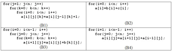
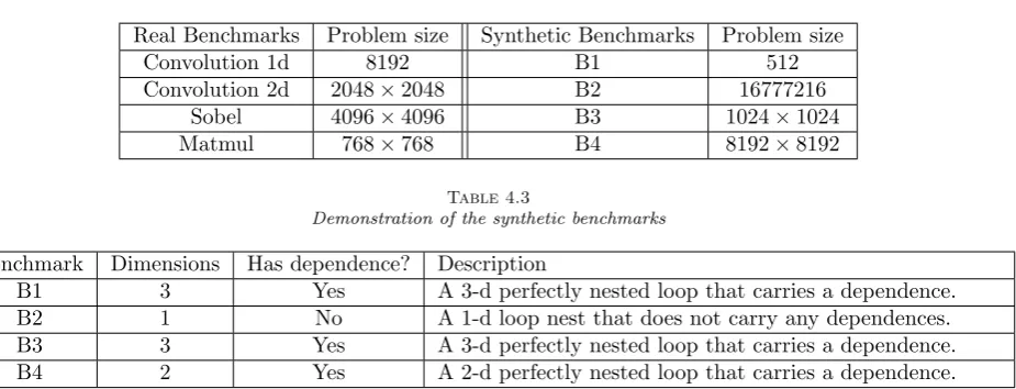
Benchmarks. To test the effectiveness of the proposed parallelization and vectorization technique, we use four data-intensive real benchmarks: matrix multiplication, one-dimensional convolution, two-dimensional convolution, and Sobel filter. Matrix multiplication is the core mechanism in linear algebra applications such as image processing, and physical or economic simulations, and improving it can be very useful in real life applications. Both one and two-dimensional convolutions are very regular in Digital Signal Processing (DSP) field and finally, Sobel filter is an application of two-dimensional convolution. The another set contains four synthetic benchmarks covering four cases that are usual in the scientific applications. Table 4.3 demonstrate each case and the synthetic benchmark covering it. This set of benchmarks is listed in Table 4.1. All the benchmarks use single precision floating point operations. Table 4.2 shows problem sizes used in the benchmarks. All array sizes used in the benchmarks were set to be significantly larger than last level cache of the hardware platform.
4.2. Experimental Results. For the given problem sizes in the Table 4.2, the parallelized and vectorized codes are generated by the PVL method. The experimental evaluations in the follow show that, as theoretically
Table 4.1
Table 4.2
The Problem sizes used in benchmarks
Real Benchmarks Problem size Synthetic Benchmarks Problem size
Convolution 1d 8192 B1 512
Convolution 2d 2048×2048 B2 16777216
Sobel 4096×4096 B3 1024×1024
Matmul 768×768 B4 8192×8192
Table 4.3
Demonstration of the synthetic benchmarks
Benchmark Dimensions Has dependence? Description
B1 3 Yes A 3-d perfectly nested loop that carries a dependence.
B2 1 No A 1-d loop nest that does not carry any dependences.
B3 3 Yes A 3-d perfectly nested loop that carries a dependence.
B4 2 Yes A 2-d perfectly nested loop that carries a dependence.
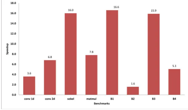
expected, when benchmarks are parallelized and vectorized using PVL method, because the PVL attempts to use both cores and SIMD short vectors to execute the benchmark, the execution time of the benchmarks reduce significantly. As a result of using all available resources of the platform, the PVL could approach to the peak performance of the underlying platform. Figures 4.1 and 4.2 show the gained speed up through the proposed approach over the sequential execution of the original programs on both systems. The average speedup of the proposed method on two and four threads (cores) is about 6.56 and 9.17, respectively. As it is clear in the proposed method, the speedup is achieved not only by multiple cores, but (1) through parallelization using multiple cores and (2) vectorization using short-vectors within each core and also (3) trying to optimize data locality to reduce cache miss. Hence, the gained speedup usually is more than number of cores.
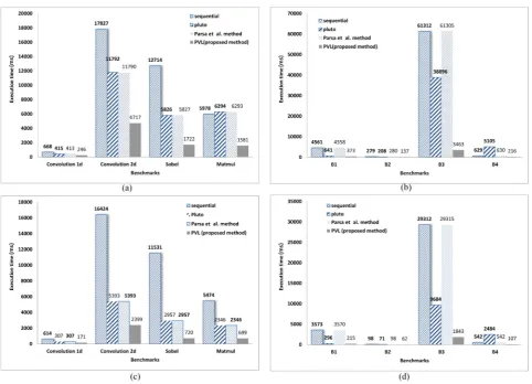
Figure 4.3 shows the execution time of the sequential, Pluto [40], Parsa et al. [22] method, and PVL (proposed method) on both sets of benchmarks on two and four cores systems. We compiled the sequential program and output of mentioned three methods using GCC compiler. Figures 4.3 (a) and 4.3 (c) are the execution time of the real benchmarks on two cores and four cores systems, respectively. Figures 4.3 (b) and 4.3 (d) are the execution time of the synthetic benchmarks on two cores and four cores systems, respectively. In all benchmarks, execution time of the PVL (proposed method) is much faster than the others.
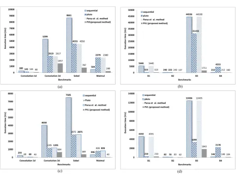
4.3. Execution with -O3 flag. The underlying hardware architecture of the proposed method and both compared methods are modern multi-core architectures with given sources for parallel and vector executions: cores and short-vectors. However, both compared methods are giving priority to the cores and postponing vectorization. We claim that in order to have best execution time, both cores and short-vectors have to be given enough importance. So, we try to find loop transformation proper for both cores and short-vectors at the same time. In order to demonstrate our claim, we have compared the proposed method with two main research of the filed in two different scenarios: (1) at first, we have executed the results of the compared methods without any changes on the given hardware. In this scenario both of the compared methods have used only cores for execution of the benchmarks (Fig. 4.1 shows the execution times related to the this case), and (2) in order to also use short-vectors as a postponed transformation (exactly as the original intention of the compared methods), after getting results of compared methods, auto vectorization of the GCC compiler have enabled by using -O3 flag. -O3 flag of GCC not only enables auto vectorization but also it enables the highest level of safe optimizations in the compiler. By this way, both cores and short-vectors are used.
Fig. 4.1.Speedup of PVL (the proposed method) over sequential programs on Intel Dual Core CPU E2200 @ 2.20GHz CPU.
Fig. 4.2. Speedup of PVL (the proposed method) over sequential programs on Intel Core2 Quad CPU Q6600 @ 2.40GHz CPU.
to be given enough importance and also transforming schema of the PVL for modern multicore architectures is better that Pluto, and Parsa et al. approach.
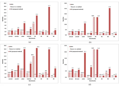
Figure 4.5 shows the speedup of the Pluto, Parsa et al. approach, and the PVL over sequential programs on two different systems with/without -O3 flag of the GCC compiler. In both sets of real and synthetic benchmarks, the speedup of the PVL is higher than the speed up of the Pluto, and Parsa et al. method. The average of the achieved speedup for the PVL (proposed method), Pluto, and Parsa et al. method over sequential in two systems with/without -O3 flag is as Table 4.4.
Figure 4.6 shows the improvement in execution time of the PVL (proposed method) over Pluto, and Parsa et al. method. Average improvement percentage in execution time of PVL over Pluto, and Parsa et al. method is as Table 4.5.
Fig. 4.3.Execution time of the sequential program, Pluto, the Parsa et al. method and the PVL (proposed method) on Intel Dual Core CPU E2200 @ 2.20GHz and Intel Core2 Quad CPU Q6600 @ 2.40GHz systems. (a) Execution of benchmarks set one on Intel Dual Core CPU E2200 @ 2.20GHz system, (b) Execution of benchmarks set two on Intel Dual Core CPU E2200 @ 2.20GHz system, (c) Execution of benchmarks set one on Intel Core2 Quad CPU Q6600 @ 2.40GHz system, and (d) Execution of benchmarks set two on Intel Core2 Quad CPU Q6600 @ 2.40GHz system
Table 4.4
The average speedup achieved by different methods
PVL (proposed method) Pluto Parsa et al. method
E2200 without -O3 6.7 2.0 1.3
E2200 with -O3 8.2 3.2 1.3
Q6600 without -O3 9.2 3.5 1.9
Q6600 with -O3 8.9 4.6 1.8
Table 4.5
The average improvement in execution time over Pluto, and Parsa et al. method
Improvement over Pluto(%) Improvement over Parsa et al. method (%)
E2200 without -O3 63.6 68.6
E2200 with -O3 61.3 64.8
Q6600 without -O3 57.8 68.8
Fig. 4.4.Execution time of the sequential program, Pluto, the Parsa et al. method, and the PVL (proposed method) on Intel Dual Core CPU E2200 @ 2.20GHz and Intel Core2 Quad CPU Q6600 @ 2.40GHz systems with -O3 flag enabled. (a) Execution of benchmarks set one on Intel Dual Core CPU E2200 @ 2.20GHz system with -O flag enalbed, (b) Execution of benchmarks set two on Intel Dual Core CPU E2200 @ 2.20GHz system with -O3 flag enabled, (c) Execution of benchmarks set one on Intel Core2 Quad CPU Q6600 @ 2.40GHz system with -O3 flag enabled, and (d) Execution of benchmarks set two on Intel Core2 Quad CPU Q6600 @ 2.40GHz system with -O3 flag enabled
the cores, (2) vectorize dependence-free loop which has contiguous data in the memory in the short-vectors within each core, and (3) improve data locality of the loops. After applying the transformation to the loop nest, intrinsic vector codes are generated to the innermost vectorizable loop using the proposed approach. Since data dependences are unavoidable in programs and they have to be satisfied as long as we want to preserve the semantic of programs, while looking for proper transformation using proposed method, we try to satisfy data dependences in the middle loops, as much as possible.
Finally, to achieve the peak performance of different hardware architectures, concentrating on both cores (outer parallelization) and data locality is not sufficient. Nowadays, widely available vector units are critical to achieving this peak performance in modern architectures. Thus, the vectorization stage should not be left to the post-transformation stage and it should be used simultaneously beside outer parallelization and data locality improvements. Although the result of the proposed method is significantly better than the state-of-the-art compiler Pluto and also the result of Parsa et al. [22], the result can be improved further by using cache configurations of the underlying system, loop tiling, and considering temporal locality.
Fig. 4.5.Speedup of Pluto, the Parsa et al. method and the PVL (proposed method) over sequential program on two core and 4 core systems. (a) Intel Dual Core CPU E2200 @ 2.20GHz system without -O3 flag, (b) Intel Dual Core CPU E2200 @ 2.20GHz system with -O3 flag enabled, (c) Intel Core2 Quad CPU Q6600 @ 2.40GHz system without -O3 flag, and (d) Intel Core2 Quad CPU Q6600 @ 2.40GHz system with -O3 flag enabled
REFERENCES
[1] U. Bondhugula,Effective automatic parallelization and locality optimization using the polyhedral model, Dissertation, (2008), The Ohio State University.
[2] L. Chai, Q. Gao, and D. K. Panda,Understanding the impact of multi-core architecture in cluster computing: A case study with intel dual-core system, In Seventh IEEE International Symposium on Cluster Computing and the Grid, (2007), pp. 471–478.
[3] Top 500 SuperComputer Sites, http://www.top500.org/. Accessed 20 December 2016. [4] G. E. Blelloch,Vector models for data-parallel computing, Cambridge: MIT press, (1990).
[5] R. Allen and K. Kennedy,Optimizing compilers for modern architectures: a dependence-based approach, San Francisco: Morgan Kaufmann, (2001).
[6] F. Franchetti,Performance portable short vector transforms, Dissertation, (2003), Karlsruhe Institute of Technology. [7] P. Bulic, and V. Gustin,An extended ANSI C for processors with a multimedia extension, International Journal of Parallel
Programming, 31 (2003), pp. 107–136.
[8] S. Raman, K. Pentkovski, and J. Keshava,Implementing streaming SIMD extensions on the Pentium III processor, IEEE micro, 20 (2000), pp. 47–57.
[9] C. Lomont,Introduction to intel advanced vector extensions, Intel White Paper, (2011), pp. 1–21.
[10] K. Stock, T. Henretty, I. Murugandi, P. Sadayappan, and R. Harrison,Model-driven simd code generation for a multi-resolution tensor kernel, In Parallel & Distributed Processing Symposium (IPDPS), IEEE, 51 (2011), pp. 1058–1067. [11] J. M. Cebrian, M. Jahre, and L. Natvig,ParVec: vectorizing the PARSEC benchmark suite, Computing Journal, 97
Fig. 4.6. Improvements in execution time over Pluto, and Parsa et al. method on two core and 4 core systems. (a) Intel Dual Core CPU E2200 @ 2.20GHz system without -O3 flag, (b) Intel Dual Core CPU E2200 @ 2.20GHz system with -O3 flag enabled, (c) Intel Core2 Quad CPU Q6600 @ 2.40GHz system without -O3 flag and (d) Intel Core2 Quad CPU Q6600 @ 2.40GHz system with -O3 flag enabled
[12] L. N. Pouchet,When iterative optimization meets the polyhedral model: one-dimensional date, Dissertation, (2006), Uni-versity of Paris-Sud XI.
[13] M. W. Benabderrahmane , L. N. Pouchet, A. Cohen, and C. Bastoul,The polyhedral model is more widely applicable than you think, In Compiler Construction, (2010), pp. 283–303.
[14] S. Girbal, N. Vasilache, C. Bastoul, A. Cohen, D. Parello, M. Sigler, and O. Temam,Semi-automatic composition of loop transformations for deep parallelism and memory hierarchies, International Journal of Parallel Programming, 34 (2006), pp. 261–317.
[15] C. Bastoul, Code generation in the polyhedral model is easier than you think, In Proceedings of the 13th International Conference on Parallel Architectures and Compilation Techniques, (2004), pp. 7–16.
[16] J. Xue,Loop tiling for parallelism, Springer Science & Business Media, (2000).
[17] R. Allen and K. Kennedy,Vector register allocation, IEEE Transactions on Computers, 41 (1992), pp. 1290–1317. [18] R. Xu, S. Chandrasekaran, X. Tian, and B. Chapman,An Analytical Model-Based Auto-tuning Framework for
Locality-Aware Loop Scheduling, In International Conference on High Performance Computing, (2016), pp. 3–20.
[19] D. Unat, T. Nguyen, W. Farooqi, M. N. Bastem, G. Michelogiannakis, and J. Shalf,Tida: High-level programming abstractions for data locality management, In International Conference on High Performance Computing, (2016), pp. 116– 135.
[20] S. Naci,Optimizing Inter-Nest Data Locality Using Loop Splitting and Reordering, In Parallel and Distributed Processing Symposium, (2007), pp. 1–8.
[21] O. Ozturk,Data locality and parallelism optimization using a constraint-based approach, Journal of Parallel and Distributed Computing, 71 (2011), pp. 280–287.
[23] W. Bielecki, and M. Palkowski,Loop Nest Tiling for Image Processing and Communication Applications, In International Multi-Conference on Advanced Computer Systems, (2016), pp. 305–314.
[24] K. Qiu, Y. Ni, W. Zhang, J. Wang, X. Wu, C. J. Xue, and T. Li,An adaptive Non-Uniform Loop Tiling for DMA-based bulk data transfers on many-core processor, In Computer Design (ICCD), (2016), pp. 9–16.
[25] S. Parsa, S. Lotfi,A new genetic algorithm for loop tiling, The Journal of Supercomputing, 37 (2006), pp. 249–269. [26] S. Krishnamoorthy, M. Baskaran, U. Bondhugula, J. Ramanujam, A. Rountev, and P. Sadayappan,Effective
auto-matic parallelization of stencil computations, In ACM Sigplan Notices, 42 (2007), pp. 235–244.
[27] U. Bondhugula, M. Baskaran, S. Krishnamoorthy, J. Ramanujam, A. Rountev, and P. Sadayappan,Automatic trans-formations for communication-minimized parallelization and locality optimization in the polyhedral model, In Compiler Construction, (2008), pp. 132–146.
[28] V. Bandishti, I. Pananilath, and U. Bondhugula,Tiling stencil computations to maximize parallelism, In Proceedings of the International Conference on High Performance Computing, Networking, Storage and Analysis, (2012), pp. 40–51. [29] M. Baskaran, B. Pradelle, B. Meister, A. Konstantinidis, and R. Lethin,Automatic code generation and data
man-agement for an asynchronous task-based runtime, In Proceedings of the 5th Workshop on Extreme-Scale Programming Tools, (2016), pp. 34–41.
[30] J. Cong, M. Huang, P. Pan, Y. Wang, and P Zhang,Source-to-source optimization for HLS, In FPGAs for Software Programmers, (2016), pp. 137–163.
[31] Q. Lu, C. Alias, U. Bondhugula, T. Henretty, S. Krishnamoorthy, J. Ramanujam, and T. F. Ngai, Data layout transformation for enhancing data locality on nuca chip multiprocessors, In Parallel Architectures and Compilation Techniques, (2009), pp. 348–357.
[32] B. Jang, P. Mistry, D. Schaa, R. Dominguez, and D. Kaeli,Data transformations enabling loop vectorization on multi-threaded data parallel architectures, In ACM Sigplan Notices 45 (2010), pp. 353–354.
[33] A. Krechel, H. J. Plum, and K. Stuben, Parallelization and vectorization aspects of the solution of tridiagonal linear systems, Parallel Computing, 14 (1990), pp. 31–49.
[34] C. Aykanat, F. Ozguner, and D. S. Scott, Vectorization and parallelization of the conjugate gradient algorithm on hypercube-connected vector processors, Microprocessing and Microprogramming, 29 (1990), pp. 67–82.
[35] J. Crawford, Z. Eldredge, and G. A. Parker, Using vectorization and parallelization to improve the application of the APH hamiltonian in reactive scattering, In Computational Science and Its Applications ICCSA, Springer Berlin Heidelberg, (2013), pp. 16–30.
[36] L. N. Pouchet, U. Bondhugula, C. Bastoul, A. Cohen, J. Ramanujam, P. Sadayappan, and N. Vasilache, Loop transformations: convexity, pruning and optimization, In ACM SIGPLAN Notices, 46 (2011), pp. 549–562.
[37] P. Feautrier,Some efficient solutions to the affine scheduling problem. Part II. Multidimensional time, International journal of parallel programming, 21 (1992), pp. 389–420.
[38] R. Penrose,A generalized inverse for matrices, In Mathematical proceedings of the Cambridge philosophical society, 51 (1955), pp. 406–413.
[39] S. Pop, A. Cohen, C. Bastoul, S. Girbal, G. A. Silber, and N. Vasilache,GRAPHITE: Loop optimizations based on the polyhedral model for GCC, 4th GCC Developer’s Summit, (2006), pp. 179–198.
[40] PLUTO - An automatic parallelizer and locality optimizer for affine loop nests, http://pluto-compiler.sourceforge.net/
Edited by: Dana Petcu
Received: December 2, 2016
![Fig. 3.1. The binary expression tree of y[i] = y[i]+b[j]×x[i+j]](https://thumb-us.123doks.com/thumbv2/123dok_us/8745592.1747237/12.595.250.347.125.187/fig-binary-expression-tree-y-i-y-i.webp)