The optimization model of the vendor selection for the joint procurement from a total cost of ownership perspective

JIEM, 2015 – 8(4): 1251-1269 – Online ISSN: 2013-0953 – Print ISSN: 2013-8423 http://dx.doi.org/10.3926/jiem.1551

The Optimization Model of the Vendor Selection for the Joint

Procurement from a Total Cost of Ownership Perspective

Fu-Bin Pan

School of Management, Xiamen University of Technology(China)

[email protected]

Received: June 2015 Accepted: September 2015

Abstract:

Purpose: This paper is an attempt to establish the mathematical programming model of the

vendor selection for the joint procurement from a total cost of ownership perspective.

Design/methodology/approach: Fuzzy genetic algorithm is employed to solve the model,

and the data set of the ball bearings purchasing problem is illustrated as a numerical analysis.

Findings: According to the results, it can be seen that the performance of the optimization

model is pretty good and can reduce the total costs of the procurement.

Originality/value: The contribution of this paper is threefold. First, a literature review and

classification of the published vendor selection models is shown in this paper. Second, a

mathematical programming model of the vendor selection for the joint procurement from a

total cost of ownership perspective is established. Third, an empirical study is displayed to

illustrate the application of the proposed model to evaluate and identify the best vendors for

ball bearing procurement, and the results show that it could reduce the total costs as much as

twenty percent after the optimization.

1. Introduction

Vendor/supplier selection is one of the most important activities of acquisition since the results have a great impact on the quality of goods and performance of the supply chains (Chen, Lin & Huang, 2006; Castro, Gómez & Franco, 2009; Thrulogachantar & Zailani, 2011). It is also necessary to anticipate the evaluation of performance of the suppliers to establish a collaborative relationship (Ha, Park & Cho, 2011). Essentially, vendor selection is a decision process regarding to reducing the initial set of potential suppliers to the final choices (Boer, Labro & Morlacchi, 2001; Wu & Barnes, 2011). Procurement management is an extremely important activity in supply chain management (Masella & Rangone, 2000; Azoulay-Schwartz, Kraus & Wilkenfeld, 2004). As elaborated later in the detailed review of literature, within the domain of procurement, vendor selection is one of the highly researched problems due to the high degree of complexity and criticality of the domain. The evaluation criteria may be different there would be divergent vendor evaluation criteria for a specific procurement decision making process. The presence of multiple such divergent and multidimensional criteria makes the supplier selection problem very complex.

Although a wide variety of decision support theories have been illustrated in the domain of vendor selection, it is necessary to make quantitative researches in terms of the vendor selection. However, most of the current literature focused on the vendor selection from one factory, there has been limited research focused on the vendor selection for the joint procurement from more than one factory belong to one enterprise group from a total cost of ownership perspective, which is the primary motivation of this research.

The paper is organized as follows. The next section introduces the related literature about supplier/vendor selection. Following is the mathematical programming model of the vendor selection for the joint procurement from a total cost of ownership perspective. Section 4 describes the fuzzy genetic algorithm applied in this research. In the following section, the numerical analysis is illustrated. Finally, the suggestions for the joint procurement in terms of reducing the total cost of the value chain of the firm are identified and discussed along with the related managerial implications.

2. Literature Review

2.1. Vendor Selection

• make or buy,

• supplier selection,

• contract negotiation,

• design collaboration,

• procurement, and

• sourcing analysis.

Aksoy and Ozturk (Aksoy & Ozturk, 2011) investigate the supplier selection and performance evaluation in just-in-time production environments.

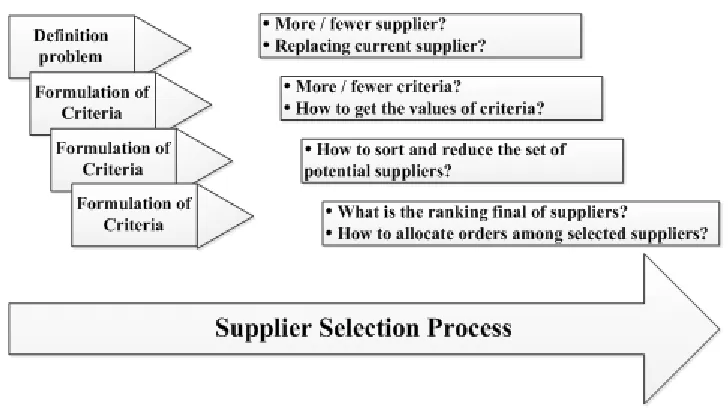
Figure 1. The supplier selection framework

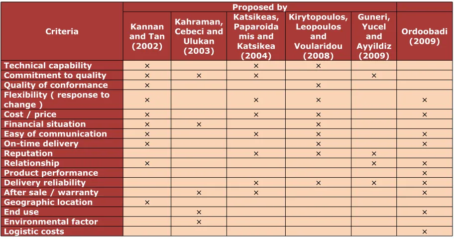
includes purchasing strategy system, supplier selection system and supplier management system is proposed (Lee, Ha & Kim, 2001). Lee (Lee, 2009) provides a fuzzy supplier selection model with the consideration of benefits, opportunities, costs and risks. Table 1 shows some important criteria for vendor selection.

Criteria Proposed by Kannan and Tan (2002) Kahraman, Cebeci and Ulukan (2003) Katsikeas, Paparoida mis and Katsikea (2004) Kirytopoulos, Leopoulos and Voularidou (2008) Guneri, Yucel and Ayyildiz (2009) Ordoobadi (2009)

Technical capability × × ×

Commitment to quality × × × ×

Quality of conformance × ×

Flexibility ( response to

change ) × × × ×

Cost / price × × × ×

Financial situation × × ×

Easy of communication × × × ×

On-time delivery × × ×

Reputation × × ×

Relationship × × ×

Product performance ×

Delivery reliability × × × ×

After sale / warranty × × ×

Geographic location ×

End use × ×

Environmental factor ×

Logistic costs ×

Table 1. Supplier performance criteria according to selected authors

2.2. The Total Cost of Ownership Approach

The concept of Total Cost of Ownership (TCO) refers to all costs associated with the procurement process throughout the entire value chain of the firm. The costs of the acquisition and subsequent use of an item or service that is to be purchased is determined. The approach goes beyond price to consider all costs over the items’ entire life such as those related to service, quality, delivery, administration, communication, failure, maintenance, etc. (Ellram, 1994; Ellram, 1995). The analysis of costs throughout the entire value chain of a company is an important topic in today’s management accounting literature (Shank & Govindarajan, 1992).

There are some researches elaborate on the application of the TCO concept in procurement management (Carr & Ittner, 1992; Cavinato, 1992). A hierarchical structure in activities with respect to the procurement problem is identified as follows:

• the supplier level activities,

• the order level activities and

The supplier level costs refer to the costs incurred and conditions imposed whenever the purchasing company actually uses the supplier over the decision horizon. For example, the costs on the supplier level include a quality audit cost incurred by the buyer for the evaluation of a supplier, the cost of a dedicated purchasing manager and additional research and development costs due to use a particular supplier. The order level parameters indicate costs incurred and conditions imposed each time an order is placed with a particular supplier and include, amongst others, costs associated with reception, transportation, invoicing, ordering and receiving credit notes. The unit level costs includes the costs related to the units of the products for which the procurement decision has to be made, for instance, price, internal failure, external failure and inventory holding.

3. Vendor Selection Mathematical Model

In this section, we present the mathematical programming decision model that was used for the determination of an optimal sourcing strategy for the ball bearing product group. The only assumption used is the fact that the company can place at most one order per time period with each supplier. This assumption is not restrictive, however, as the typical order frequency could determine the length of the time bucket to be a month, a week or even a day.

3.1 Description of the Problem

This model is based on the consideration of the joint procurement of all the factories in the same enterprise group, and the model consumptions are as following:

• The cost of ordering per order of the suppliers and the price of the ball bearing in the

procurement process is irrelevant for the factories they serviced during the procurement, but the capacity and the price of the logistic to different suppliers from the same factory may vary.

• The requirements for the ball bearing may be different for the factories, and the

3.2. Symbols of the Model

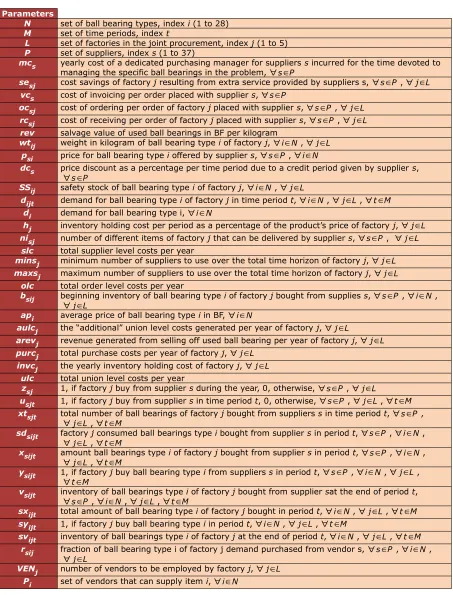
Before starting the model, symbols of the model are shown in Table 2.

Parameters

N set of ball bearing types, index i (1 to 28)

M set of time periods, index t

L set of factories in the joint procurement, index j (1 to 5)

P set of suppliers, index s (1 to 37)

mc_s yearly cost of a dedicated purchasing manager for suppliers s incurred for the time devoted to managing the specific ball bearings in the problem,∀s∈P

se_sj cost savings of factory j resulting from extra service provided by suppliers s,∀s∈P ,∀j∈L vc_s cost of invoicing per order placed with supplier s,∀s∈P

oc_sj cost of ordering per order of factory j placed with supplier s,∀s∈P,∀j∈L rc_sj cost of receiving per order of factory j placed with supplier s,∀s∈P ,∀j∈L rev salvage value of used ball bearings in BF per kilogram

wt_ij weight in kilogram of ball bearing type i of factory j,∀i∈N,∀j∈L p_si price for ball bearing type i offered by supplier s,∀s∈P ,∀i∈N

dc_s price discount as a percentage per time period due to a credit period given by supplier s,

∀s∈P

SS_ij safety stock of ball bearing type i of factory j,∀i∈N,∀j∈L

d_ijt demand for ball bearing type i of factory j in time period t,∀i∈N,∀j∈L,∀t∈M d_i demand for ball bearing type i,∀i∈N

h_j inventory holding cost per period as a percentage of the product’s price of factory j,∀j∈L ni_sj number of different items of factory j that can be delivered by supplier s,∀s∈P , ∀j∈L

slc total supplier level costs per year

mins_j minimum number of suppliers to use over the total time horizon of factory j,∀j∈L maxs_j maximum number of suppliers to use over the total time horizon of factory j,∀j∈L

olc total order level costs per year

b_sij beginning inventory of ball bearing type i of factory j bought from supplies s,∀s∈P ,∀i∈N,

∀j∈L

ap_i average price of ball bearing type i in BF,∀i∈N

aulc_j the “additional” union level costs generated per year of factory j,∀j∈L

arev_j revenue generated from selling off used ball bearing per year of factory j,∀j∈L purc_j total purchase costs per year of factory j,∀j∈L

invc_j the yearly inventory holding cost of factory j,∀j∈L ulc total union level costs per year

z_sj 1, if factory j buy from supplier s during the year, 0, otherwise,∀s∈P ,∀j∈L

u_sjt 1, if factory j buy from supplier s in time period t, 0, otherwise,∀s∈P ,∀j∈L,∀t∈M xt_sjt total number of ball bearings of factory j bought from suppliers s in time period t,∀s∈P ,

∀j∈L,∀t∈M

sd_sijt factory j consumed ball bearings type i bought from supplier s in period t,∀s∈P ,∀i∈N,

∀j∈L,∀t∈M

x_sijt amount ball bearings type i of factory j bought from supplier s in period t,∀s∈P ,∀i∈N,

∀j∈L,∀t∈M

y_sijt 1, if factory j buy ball bearing type i from suppliers s in period t,∀s∈P ,∀i∈N,∀j∈L,

∀t∈M

v_sijt inventory of ball bearings type i of factory j bought from supplier sat the end of period t,

∀s∈P,∀i∈N,∀j∈L,∀t∈M

sx_ijt total amount of ball bearing type i of factory j bought in period t,∀i∈N,∀j∈L,∀t∈M sy_ijt 1, if factory j buy ball bearing type i in period t,∀i∈N,∀j∈L,∀t∈M

sv_ijt inventory of ball bearings type i of factory j at the end of period t,∀i∈N,∀j∈L,∀t∈M r_sij fraction of ball bearing type i of factory j demand purchased from vendor s,∀s∈P ,∀i∈N,

∀j∈L

VEN_j number of vendors to be employed by factory j,∀j∈L P_i set of vendors that can supply item i,∀i∈N

3.3. Mathematical Model

With the notation given above, the mathematical decision model is described as follow, and the objective of the model is based on the research of Degraeve and Roodhooft (1999):

Min slc + olc + ulc (1)

slc=

∑

s∈P

∑

mc_sz_sj−

∑

j∈L

(

∑

(

se_sj

∑

i∈Nt

∑

p_sijx_sijt

)

)

olc=

∑

s∈P

∑

∑

(

vc_s+oc_sj+rc_sj

)

ulc=

∑

j∈L

(

purc_j+invc_j−arev_j

)

purc_j=

∑

s∈P

∑

∑

ps_si

(

)

invc_j=

∑

s∈P

∑

∑

h ps_siv_sijt+

∑

i∈N

37h_jap_iSS_ij, ∀j∈L ₍₆₎

arec_j=

∑

i∈Nt

∑

rev wt_ijd_ij ∀j∈L ₍₇₎

∑

s∈P

∑

sd_sijt=d_ijt, ∀j∈L ₍₈₎

b_sij+x_sijt−v_sijt=sd_sijt ∀s∈P, ∀i∈N, ∀j∈L, t=1 (9)

v_sij(t−1)+x_sijt−v_sijt=sd_sijt ∀s∈P, ∀i∈N, ∀j∈L, ∀t∈M∖

{

}

v_sij≤

∑

l∈M∖{1,... ,t}

d_ijly_sijt, ∀s∈P, ∀i∈N, ∀j∈L, ∀t∈M ₍₁₁₎

∑

i∈N

x_sijt=xt_sjt, ∀s∈P, ∀j∈L, ∀t∈M ₍₁₂₎

xt_sij≤

∑

i∈N

u_sjt

(

∑

l∈M∖{1,... ,t}

d_ijl

)

u_sij≤

∑

i∈N

y_sijt, ∀s∈P, ∀j∈L, ∀t∈M ₍₁₄₎

y_sjit≤u_sjt, ∀s∈P, ∀i∈N, ∀j∈L, ∀t∈M (15)

∑

s∈P

z_sj≥mins_j ∀j∈L ₍₁₆₎

∑

s∈P

z_sj≤

∑

t∈M

u_sjt, ∀s∈P, ∀j∈L ₍₁₈₎

u_sjt≤z_sj, ∀s∈P, ∀j∈L, ∀t∈M (19)

z_sj∈

{

}

u_sjt∈

{

}

y_sijt∈

{

}

∑

s∈P

x_sijt=sx_ijt, ∀i∈N, ∀j∈L, ∀t∈M ₍₂₃₎

∑

s∈P

v_sijt=sv_ijt, ∀i∈N, ∀j∈L, ∀t∈M ₍₂₄₎

sx_ijt≤

(

∑

l∈M∖{1,... ,t}

d_ijl

)

sy_ijt≤

∑

s∈P

y_sijt, ∀i∈N, ∀j∈L, ∀t∈M ₍₂₆₎

y_sijt≤sy_ijt, ∀sP, ∀iN, ∀jL, ∀tM (27)

∑

t∈C

sx_ijt≤

∑

t∈C

sy_ijt

(

∑

g

d_ijr

)

{

}

The calculation methods of costs are given by Equation (1) - Equation (6). Equation (1) is objective function, which is used to evaluate alternative procurement policies, is a minimization of the total cost of ownership and reflects net prices and resources consumed by the activities in the three hierarchical levels distinguished. Equation (2) is the supplier level cost. The supplier level costs are incurred whenever the purchasing company actually uses supplier s

over the planning horizon, i.e. zsj = 1. A dedicated purchasing manager can be put to some

alternative use if supplier s is not chosen, i.e. zsj = 0. Equation (3) is the order level cost. The

order level costs are incurred in those time periods t when an order is placed with a particular

supplier, i.e. usjt = 1. They consist of the invoice cost and the ordering cost when factory j

purchasing from supplier s. Equation (4) is the union level cost. The union level costs consist of

the inventory holding cost. The inventory holding cost applies to the total amount of factory j’s

ball bearings type i of supplier s held in inventory in each time period t, vsijt. Equation (7) is the

additional revenue. Additional revenue is generated by selling off used ball bearings which can partly be recycled. The salvage value which essentially includes the value of the steel is applied

to the weight and the union consumed in time period t, dijt.

The constraints relevant to the procurement problem of the ball bearing are given by Equation (8) ~ Equation (28). Equation (8) will determine the consumption of ball bearings type i that

factory j bought from each supplier in each time period of the planning horizon, sdsijt. Equation

(9) is the consumption of ball bearing type i from each supplier in the first time period, sdsijt, t =

1. Equation (10) model the consumption of products from each supplier in later time periods,

sdsijt. Equation (11) essentially model the logical relationship between the ordering, ysijt, and

the order quantity variables, xsijt. Equation (12) is the total amount of ball bearings of any type

that factory j bought from a vendor s in time period t, xtsjt. Equation (13) model the proper

relationship between the ordering variables, usjt, and the total amount ordered. The logical

conditions Equation (14) and Equation (15) are required to correctly define the ordering

variables usjt which are used in the objective function at the order level. The conditions

Equation (16) and Equation (17) force the purchasing plan to have at least the minimum number, mins, and at most the maximum number, maxs, of suppliers over the complete time

horizon. Using constraint (18), the decision variable zsj will be equal to 0, if the model suggests

factory j not to buy from the supplier s, while constraint (19) forces zsj to be equal to 1, if

during some time period t, an order has been placed with supplier s. To conclude the model

specification, constraints (20) - (22), impose the proper integrality and non negativity conditions that apply to the decision variables. Equation (23) and Equation (24) define the

total quantity bought and inventory of factory j’s ball bearing type i in time period t.

Inequalities (25) model the relationship between the total amount ordered and the ordering decision while inequalities (26) and (27) enforce the logical relationships among the 0/1 decision variables involved. Cutting planes (28) represent facet defining inequalities for the lot size polytope (8) - (10).

4. Improved Fuzzy Genetic Algorithm

Vendor selection is one of combinational optimization problems. As shown in this section, the combinatorial problem formulated in section 3 can be reduced to a standard knapsack model, and thus is NP-complete problem. An improved fuzzy genetic algorithm is proposed to get the better solution in limited time.

This computation is followed by running GA operations such as selection, crossover and mutation. Selection retains the successful solutions (operator chains), whereas crossover and mutation are included to try to diversify the remaining candidate solutions for the next generations. In the next step, the parameters of the GA are updated by an adaptive fuzzy logic controller to improve the algorithm’s performance. The newly adjusted parameters are then used in the next generation. This evolutionary process is repeated until a predefined number of generations is reached.

The performance of GA is quite sensitive to control parameters. A tendency for all of the population to converge to a single suboptimal solution is also possible given a low mutation rate. If all of the members of the population are very similar, the crossover operator has little function and mutation turns out to be the primary operator (Jafari, Mashohor & Vamamkhasti, 2011). This negative effect triggers the problem of premature convergence, where the solving procedure is trapped in a suboptimal state and most of the operators are unable to generate offspring that surpass their parents any more. The use of fuzzy logic controllers to adapt GA parameters is one possible solution to overcome these impediments and improve the performance of the GA.

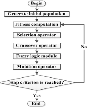
In this study, we propose an adaptive fuzzy logic-based genetic approach to the detection of vendor selection problem. As the approach’s major novelty, an adaptive-fuzzy logic module is integrated with the conventional GA in an attempt to improve the performance of the GA and reduce the premature convergence problem by adjusting the algorithm’s parameters. The flow chart of fuzzy logic genetic algorithm is shown in Figure 2.

4.1. Design of GA

4.1.1. Encoding

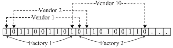
Traditionally, a chromosome is a sequence of binary digits, which represents a solution in the problem domain. The bits of the chromosome are referred to as its genes and are mapped to parts of a solution. Binary digit encoding method is used in this paper. There is an example that includes two factories and ten vendors, and the binary digit encoding of this example is shown in Figure 3.

Figure 3. Binary digit encoding

4.1.2. Fitness Function

Usually, the reciprocal of objective function is chose as fitness function. But the fitness value will be small and can’t be adjust. The difference of fitness value in different problems is greatly, so a new fitness function is proposed as follow:

tc/(slc + olc + ulc) (29)

tc is the maximum value of Equation (1).

4.1.3. Selection Operator

Binary tournament selection: In this selection process, two individuals are selected at random from the population and the fittest one is selected for reproduction.

4.1.4. Crossover Operator

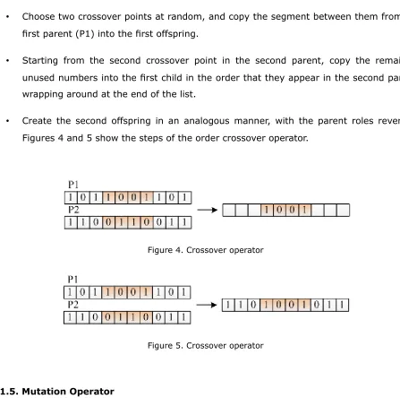
in the second parent, copy the elements to the offspring in the order they appear in the second parent, avoiding repetition. The second offspring is created in the same way, reversing the roles of the parents. The steps are shown:

• Choose two crossover points at random, and copy the segment between them from the

first parent (P1) into the first offspring.

• Starting from the second crossover point in the second parent, copy the remaining

unused numbers into the first child in the order that they appear in the second parent, wrapping around at the end of the list.

• Create the second offspring in an analogous manner, with the parent roles reversed.

Figures 4 and 5 show the steps of the order crossover operator.

Figure 4. Crossover operator

Figure 5. Crossover operator

4.1.5. Mutation Operator

Invert mutation: This operator works by randomly selecting two positions in the string and reversing the order in which the values appear between those positions (Figure 6).

Every chromosome in the population has a certain probability Pm to participate in the mutation operation. In next section, an adaptive-fuzzy logic module will be proposed to adjust the mutation probability.

The crossover and mutation operators described before require the selection of two indices in the genotype. Usually this choice is made at random, however we remark that the problem we are treating has a very special feature that can be exploited: changes in the end of the genotype have more impact on the final drawing obtained than changes in the beginning of the genotype. The reason for this is that the first edges inserted during the planarization step hardly cause crossings, while those inserted later are the ones that cause crossings. Remember that the genotype represents the order of insertion for the planarization algorithm. Given this observation, it makes sense to bias the selection of the two indices involved in crossover and mutation operators.

4.2. Adaptive-fuzzy Logic Module

The fuzzy logic module is composed of fuzzification, fuzzy inference and clarifications (Chamani, Pourshahabi & Sheikholeslam, 2013). Under the consideration that the fitness value of the chromosome has an impact on the natural evolution, an adaptive-fuzzy logic module which could adjust mutation probability according to the fitness value of the chromosome and the average fitness value of the population is proposed in this paper. The idea is as following:

• improve the mutation probability to eliminate low fitness values of individuals when

there is a significant difference between the fitness value of current chromosome and the highest fitness value of chromosome. Otherwise, lower mutation probability;

• improve the mutation probability to avoid the premature convergence when the range

of the average fitness value is small, otherwise, lower mutation probability.

F is the fitness value of current chromosome. Fr is the average fitness value of chromosomes of

generation r’s population. Fmax is the fitness value of the best chromosome in current

population. Fmin is the fitness value of the worst chromosome in current population. The output

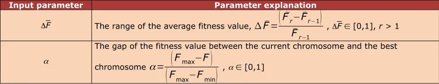
parameter is the mutation probability, and the input parameters are shown in Table 3.

Input parameter Parameter explanation

F The range of the average fitness value, ¯F=

(

)

F_r−1 , F  [0,1], r > 1

a

The gap of the fitness value between the current chromosome and the best chromosomea=

(

)

(

)

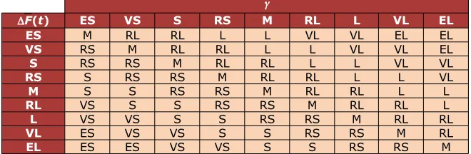
There are nine sematic values in the fuzzy logic module, which ES means extremely small, VS means very small, S means small, RS means relatively small, M means medium, RL means relatively lager, L means lager, VL means very lager and EL means extremely lager. The triangle membership function is used in this paper. According to the sematic value and triangle membership function, we can get the graphic of membership function as shown in Figure 7.

Figure 7. The membership function graphic of input and output parameter

According to the fuzzy logic and the membership, we can get the fuzzy logic rules as shown in Table 4.

g

F(t) ES VS S RS M RL L VL EL

ES M RL RL L L VL VL EL EL

VS RS M RL RL L L VL VL EL

S RS RS M RL RL L L VL VL

RS S RS RS M RL RL L L VL

M S S RS RS M RL RL L L

RL VS S S RS RS M RL RL L

L VS VS S S RS RS M RL RL

VL ES VS VS S S RS RS M RL

EL ES ES VS VS S S RS RS M

Table 4. The fuzzy logic rules of mutation probability

5. Numerical Analysis

In this section, an empirical study is displayed to illustrate the application of the proposed model to evaluate and identify the best vendors for conducting the ball bearing in real world case.

5.1 Background and Problem Descriptions

The M corporation has been used ball bearing as one of the materials since the begging of 1999. With the rapidly development of M corporation, the demand of the ball bearing is increasing, so M corporation needs to purchase more than ten million ton ball bearing from the suppliers. This corporation asks the subsidiary companies to reduce the costs in order to be competitive, while as one of the major materials, the total costs of the ball bearing procurement has a large proportion of the operations costs, which makes the M corporation to reduce the total costs of the ball bearing through optimization the vendor selection and the purchasing plan.

5.2. Data Collection

There are five subsidiary companies in M corporation purchasing ball bearing from thirty-seven suppliers, and the time period for the ball bearing procurement is one month. These five subsidiary companies shall submit their orders for the ball bearing to the corporation, and then the corporation concentrates the orders for joint procurement. The orders (before optimization) from January 2014 to October are collected from M, and then the numerical analysis is illustrated by substituting the numbers into the model established in this research to identify the optimal solution for the procurement in terms of the vendor selection and the purchasing plan.

5.3. Result of numerical analysis

The results of the numerical analysis of the purchasing cost are shown in Table 5. The validity of the model and algorithm are tested by comparing the costs before and after optimization. Under the consideration of the confidentiality of the enterprise data, not all the results are shown in Table 5 except for the vendor number, quantities purchased and the total costs.

Month numberVendor Quantities (milliontons) Cost (million dollar) before after before after before after January 32 28 0.8314 0.8315 121.8250 121.7482

February 31 30 0.8542 0.8540 130.3936 129.7482

March 32 30 0.9167 0.9168 142.2443 141.9940

April 34 32 0.9597 0.9598 143.1680 143.1254

May 33 31 1.0821 1.0821 160.3997 159.6855

June 35 32 1.0536 1.0536 156.7125 156.6598

July 35 33 1.1765 1.1766 171.0749 170.7364

August 36 33 1.1379 1.1378 165.4165 165.1630

September 37 34 1.2674 1.2675 183.4435 183.3819

October 36 32 1.0317 1.0317 154.1257 153.5582

Total 341 315 10.3112 10.3114 1528.804 1525.801

From the comparison results above, it can be seen that the quantities purchased after the optimization is no less than that before optimization, but the total costs has been reduced in each time period of the procurement. Take the order of May 2014 for example, 0.7142 million dollars is reduced comparing with the cost before optimization. 3.003 million dollar is reduced during the ten month totally, that is, average 0.3003 million dollars cost reductions monthly, which is as high as nearly twenty percent of cost reductions.

6. Conclusions and Suggestions for Future Research

This study is focused on establishing the mathematical programming model of the vendor selection for the joint procurement from more than one factory belong to one enterprise group from a total cost of ownership perspective, which is an improved model of vendor selection for the joint procurement from one factory. Adaptive-fuzzy genetic algorithm is employed to solve the model, and the data set of the ball bearings purchasing problem is illustrated as a numerical analysis. According to the results, it can be seen that the performance of the optimization model is pretty good and can reduce the total costs of the procurement.

The contribution of this paper is threefold. First, a mathematical programming model of the vendor selection for the joint procurement from a total cost of ownership perspective is established; second, an improved adaptive-fuzzy genetic algorithm is employed to solve the model; third, an empirical study is displayed to illustrate the application of the proposed model to evaluate and identify the best vendors for ball bearing procurement, and the results show that it could reduce the total costs as much as twenty percent after the optimization.

Future research should be conducted in developing mu multiple item mathematical programming vendor selection models with inventory management, since the simultaneous decision to select vendors and to determine order quantities seems to be saving on TCO. A second fruitful path for future research is to introduce uncertainty with respect to requirements, deliveries, quality, prices etc. in decision models. Thirdly, the same methodology can also be applied to other real life data sets to check whether the conclusions remain.

Acknowledgments

References

Aksoy, A., & Ozturk, N. (2011). Supplier selection and performance evaluation in just-in-time

production environments. Expert Systems with Applications, 38, 635 1-63 59.

http://dx.doi.org/10.1016/j.eswa.2010.11.104

Azoulay-Schwartz, R., Kraus, S., & Wilkenfeld, J. (2004). Exploitation vs. exploration: Choosing

a supplier in an environment of incomplete information. Decision Support Systems, 38(1),

1-18. http://dx.doi.org/10.1016/S0167-9236(03)00061-7

Boer, L.D., Labro, E., & Morlacchi, P. (2001). A review of methods supporting supplier selection.

European Journal of Purchasing Supply Management, 7, 75-89.

http://dx.doi.org/10.1016/S0969-7012(00)00028-9

Carr, L., & Ittner, C. (1992). Measuring the cost of ownership. Journal of Cost Management,

6(3), 7-13.

Castro, W., Gómez, O., & Franco, L. (2009). Selección de proveedores: una aproximación al

estado del arte. Cuaderno de Administración, 22, 145-167.

Cavinato, J. (1992). A total cost/value model for supply chain competitiveness. Journal of

Business Logistics, 13(2), 285-301.

Chamani, M.R., Pourshahabi, S., & Sheikholeslam, F. (2013). Fuzzy genetic algorithm approach

for optimization of surge tanks. Scientia Iranica, 20(2), 278-285.

Chan, F., & Chan, H. (2004). Development of the supplier selection model a case study in the

advanced technology industry. Proceedings of the Institution of Mechanical Engineers, 218,

1807-1824. http://dx.doi.org/10.1177/095440540421801213

Chang, B., Chang, C., & Wu, C. (2011). Fuzzy DEMATEL method for developing supplier

selection criteria. Expert Systems with Applications, 38, 1850-1858.

http://dx.doi.org/10.1016/j.eswa.2010.07.114

Chen, C., Lin, C., & Huang, S. (2006). A fuzzy approach for supplier evaluation and selection.

International Journal of Production Economy, 102, 289-301.

http://dx.doi.org/10.1016/j.ijpe.2005.03.009

Choy, K., Lee, W., & Lo, V. (2002). An intelligent supplier management tool for benchmarking

suppliers in outsource manufacturing. Expert Systems with Applications, 22, 213-224.

http://dx.doi.org/10.1016/S0957-4174(01)00055-0

Degraeve, Z., & Roodhooft, F. (1999). A mathematical programming approach for procurement

using activity based costing. Business Finance and Accounting, 7, 77-89.

Ding, H., Benyoucef, L., & Xie, X. (2005). A simulation optimization methodology for supplier

selection problem. International Journal of Computer Integrated Manufacturing, 18(2–3),

Ellram, L. (1994). Total Cost Modeling in Purchasing. Center for Advanced Purchasing Studies, AZ.

Ellram. L. (1995). Total cost of ownership an analysis approach for purchasing. Journal of

Physical Distribution and Logistics, 25(8), 4-23. http://dx.doi.org/10.1108/09600039510099928

Emre, S., & Mustafa, T. (2013). An adaptive fuzzy-genetic algorithm approach for building

detection using high-resolution satellite images. Computers, Environment and Urban

Systems, 39, 48-62. http://dx.doi.org/10.1016/j.compenvurbsys.2013.01.004

Francisco, R., Lauro, O., & Luiz, C. (2014). A comparison between Fuzzy AHP and Fuzzy

TOPSIS methods to supplier selection. Applied Soft Computing, 21, 194-209.

http://dx.doi.org/10.1016/j.asoc.2014.03.014

Guneri, A.F., Yucel, A., & Ayyildiz, G. (2009). An integrated fuzzy-LP approach for a supplier

selection problem in supply chain management. Expert Systems with Applications, 36,

9223-9228. http://dx.doi.org/10.1016/j.eswa.2008.12.021

Ha, B., Park, Y., & Cho, S. (2011). Suppliers’ affective trust and trust in competency in buyer.

International Journal of Operation Production Management, 31, 56-77.

http://dx.doi.org/10.1108/01443571111098744

Jafari, S.A., Mashohor, S., & Varnamkhasti, M.J. (2011).Committee neural networks with fuzzy

genetic algorithm. Journal of Petroleum Science and Engineering, 76, 217-223.

http://dx.doi.org/10.1016/j.petrol.2011.01.006

Kahraman, C., Cebeci, U., & Ulukan, Z. (2003). Multi-criteria supplier selection using fuzzy.

Logistics Information Management, 16, 382-394. http://dx.doi.org/10.1108/09576050310503367

Kannan. V.R., & Tan, K.C. (2002). Supplier selection and assessment: Their impact on business

performance. Journal of Supply Chain Manage, 38, 11-21.

http://dx.doi.org/10.1111/j.1745-493X.2002.tb00139.x

Katsikeas, C.C., Paparoidamis, N.G., & Katsikea, E. (2004). Supply source selection criteria:

The impact of supplier performance on distributor performance. Industrial Marketing

Management, 33, 755-764. http://dx.doi.org/10.1016/j.indmarman.2004.01.002

Kar, A. (2014). A Hybrid Group Decision Support System for Supplier Selection using Analytic

Hierarchy Process, Fuzzy Set Theory and Neural Network. Journal of Computational Science,

15, 231-245.

Kirytopoulos, K., Leopoulos, V., & Voulgaridou, D. (2008). Supplier selection in pharmaceutical

industry: An analytic network process approach. Benchmark International Journal, 15,

494-516. http://dx.doi.org/10.1108/14635770810887267

Lee, H. (2009). A fuzzy supplier selection model with the consideration of benefits,

opportunities, costs and risks. Expert Systems with Applications, 36, 2879-2893.

Lee, E., Ha, S., & Kim, S. (2001). Supplier selection and management system considering

relationships in supply chain management. IEEE Transactions on Engineering Management,

48(3), 307-318. http://dx.doi.org/10.1109/17.946529

Liu, F., Ding, F., & Lall, V. (2003). Using data envelopment analysis to compare suppliers for

supplier selection and performance improvement. Supply Chain Management: An

International Journal, 5(3), 143-150. http://dx.doi.org/10.1108/13598540010338893

Masella, C., & Rangone, A. (2000). A contingent approach to the design of vendor selection

systems for different types of co-operative customer/supplier relationships. International

Journal of Operations and Production Management, 20, 70-84.

http://dx.doi.org/10.1108/01443570010287044

Ordoobadi, S.M. (2009). Development of a supplier selection model using fuzzy logic. Supply

Chain Management International Journal,14, 314-327.

http://dx.doi.org/10.1108/13598540910970144

Shank, J., & Govindarajan, V. (1992). Strategic cost management: The value chain

perspective. Journal of Management Accounting Research, 4, 179-197.

Thrulogachantar, P., & Zailani, S. (2011). The influence of purchasing strategies on

manufacturing performance. Journal of Manufacturing Technology Management, 22,

641-663. http://dx.doi.org/10.1108/17410381111134482

Ware, N., Singh, S., & Banwet, D. (2014). A mixed-integer non-linear program to model

dynamic supplier selection problem. Expert system with Applications, 41(2), 671-678.

http://dx.doi.org/10.1016/j.eswa.2013.07.092

Wu, C., & Barnes, D. (2011). A literature review of decision-making models and approaches for

partner selection in agile supply chains. Journal of Purchasing Supply Management, 17,

256-274. http://dx.doi.org/10.1016/j.pursup.2011.09.002

Journal of Industrial Engineering and Management, 2015 (www.jiem.org)

Article's contents are provided on an Attribution-Non Commercial 3.0 Creative commons license. Readers are allowed to copy, distribute and communicate article's contents, provided the author's and Journal of Industrial Engineering and Management's names are included.