Memory Efficient Kernel Approximation
Si Si∗ [email protected]
Google Research
Mountain View, CA 94043, USA
Cho-Jui Hsieh [email protected]
Departments of Computer Science and Statistics University of California, Davis
Davis, CA 95616, USA
Inderjit S. Dhillon [email protected]
Department of Computer Science University of Texas at Austin Austin, TX 78701, USA
Editor:Le Song
Abstract
Scaling kernel machines to massive data sets is a major challenge due to storage and computation issues in handling large kernel matrices, that are usually dense. Recently, many papers have suggested tackling this problem by using a low-rank approximation of the kernel matrix. In this paper, we first make the observation that the structure of shift-invariant kernels changes from low-rank to block-diagonal (without any low-rank structure) when varying the scale parameter. Based on this observation, we propose a new kernel approximation framework – Memory Efficient Kernel Approximation (MEKA), which considers both low-rank and clustering structure of the kernel matrix. We show that the resulting algorithm outperforms state-of-the-art low-rank kernel approximation methods in terms of speed, approximation error, and memory usage. As an example, on the covtype dataset with half a million samples, MEKA takes around 70 seconds and uses less than 80 MB memory on a single machine to achieve 10% relative approximation error, while standard Nystr¨om approximation is about 6 times slower and uses more than 400MB memory to achieve similar approximation. We also present extensive experiments on applying MEKA to speed up kernel ridge regression.
Keywords: kernel approximation, Nystr¨om method, kernel methods
1. Introduction
Kernel methods (Sch¨olkopf and Smola, 2002) are a class of machine learning algorithms that first map samples from input space to a high-dimensional feature space. In the high-dimensional feature space, various methods can be applied depending on the machine learning task, for example, kernel support vector machine (SVM) (Cortes and Vapnik, 1995) (Hsieh, Si, and Dhillon, 2014a) and kernel ridge regression (Saunders, Gammerman, and Vovk, 1998). A key issue in scaling up kernel machines is the storage and computation
∗. This work was done before joining Google.
c
of the kernel matrix, which is usually dense. Storing the dense matrix takes O(n2) space, while computing it requiresO(n2d) operations, wherenis the number of data points andd
is the dimension. A common approach to achieve scalability is to approximate the kernel matrix using limited memory storage. This approach not only resolves the memory issue, but also speeds up kernel machine solvers, because the time complexity for using the kernel is usually proportional to the amount of memory used to represent the kernel. Most kernel approximation methods aim to form a low-rank approximation G ≈ CCT for the kernel matrixG, with C ∈Rn×k and rank kn. Although it is well known that Singular Value Decomposition (SVD) yields the best rank-kapproximation, it often cannot be applied as it requires the entire kernel matrix to be computed and stored. To overcome this issue, many methods have been proposed to approximate the best rank-kapproximation of a kernel ma-trix, including Greedy basis selection techniques (Smola and Sch¨olkopf, 2000), incomplete Cholesky decomposition (Fine and Scheinberg, 2001), and Nystr¨om methods (Williams and Seeger, 2001).
However, it is unclear whether low-rank approximation is the most memory efficient way to approximate a kernel matrix. In this paper, we first make the observation that for practically used shift-invariant kernels, the kernel structure varies from low-rank to block-diagonal as the scaling parameter γ varies from 0 to ∞. This observation suggests that even the best rank-k approximation can have extremely large approximation error when
γ is large, so it is worth exploiting the block structure of the kernel matrix. Based on this idea, we propose a Memory Efficient Kernel Approximation (MEKA) framework to approximate the kernel matrix. Our proposed framework considers and analyzes the use of clustering in the input space to efficiently exploit the block structure of shift-invariant kernels. We show that the individual blocks generated by kmeans clustering have low-rank structure, which motivates us to apply Nystr¨om low-rank approximation to each block separately. Between-cluster blocks are then approximated in a memory-efficient manner. Our approach only needs O(nk+ (ck)2) memory to store a rank-ck approximation(where
cn is the number of clusters), while traditional low-rank methods needO(nk) space to store a rank-kapproximation. Therefore, using the same amount of storage, our method can achieve lower approximation error than the commonly used low-rank methods. Moreover, our proposed method takes less computation time than other low-rank methods to achieve a given approximation error.
Theoretically, we show that under the same amount of storage, the error bound of our approach can be better than standard Nystr¨om if the gap between the k+ 1-st and
which takes more than 2700 seconds and uses more than 2 GBytes memory on the same problem.
Parts of this paper have appeared previously in (Si, Hsieh, and Dhillon, 2014a). In this paper, we provide: (1) a more detailed survey of state-of-the-art methods; (2) much more comprehensive experimental comparisons; (3) thorough investigation of the influence of the parameters in our method; (4) the application of applying the block structure of kernel matrix to speed up kernel SVM; and (5) more discussion including how to achieve stable results and solve non-psd issues in MEKA.
The rest of the paper is outlined as follows. We first present related work in Section 2. We then explain the popular Nystr¨om approximation method and present motivation for our framework in Section 3. We then show the block structure of kernel matrix and its application to speed up kernel SVM in Section 4. Our main kernel approximation algorithm MEKA is proposed and analyzed in Section 5. Experimental results are given in Section 6, and conclusion and discussion are provided in Section 7.
2. Related Research
To approximate the kernel matrix using limited memory, one common way is to use a low-rank approximation. The best low-rank-kapproximation can be obtained by the SVD, but it is computationally prohibitive when ngrows to tens of thousands. To address the scalability issue of SVD, approximate SVD solvers such as randomized SVD (Halko, Martinsson, and Tropp, 2011) have been widely used for large-scale data. To exploit the sparse structure of large-scale network data, an alternative is to apply CUR matrix decomposition (Mahoney and Drineas, 2009) that explicitly expresses the low-rank decomposition in terms of a small number of rows and columns of the original data matrix. Another way is building a hi-erarchical tree to initialize a block Lanczos algorithm to efficiently compute the spectral decomposition of large-scale graphs (Si, Shin, Dhillon, and Parlett, 2014b). Unfortunately, to approximate kernel matrices, all the above approaches need to compute the entire kernel matrix, so the time complexity is at leastO(dn2).
Many algorithms have been proposed to overcome the prohibitive time and space com-plexity of SVD for approximating kernel matrices. They can be categorized into two classes: methods that explicitly approximate kernel matrices, and methods that approximate the kernel function.
generate structured landmark points to speed up Nystr¨om approximation (Si, Hsieh, and Dhillon, 2016).
Different Nystr¨om sampling strategies are analyzed and compared in (Kumar, Mohri, and Talwalkar, 2012; Gittens and Mahoney, 2013). Besides Nystr¨om approximation, Fine and Scheinberg (2001) use the incomplete Cholesky decomposition with pivoting for ap-proximating kernel matrices, which requires O(nk2 +nkd) time for computing a rank-k
approximation. Bach and Jordan (2005) incorporate side information (labels) into the in-complete Cholesky decomposition, and show that the resulting problem can be solved with the same O(nk2 +nkd) time complexity. Finally, Achlioptas, McSherry, and Sch¨olkopf (2001) propose a sampling and reweighted approach to obtain an unbiased estimator of the kernel-vector product, and use subspace iteration to approximate the topk eigenvectors.
Approximating the kernel function. The second class of methods is to directly approximate the kernel function without computing elements of the kernel matrix, so the approximation does not depend on the data. To approximate the kernel function, a typical approach is to find a feature mapping Z :Rd→Rk where the kernel function K(x,y) can be approximated byZ(x)TZ(y). Rahimi and Recht (2007, 2008) define the random feature map for shift invariant kernel functions based on the Fourier transform. In the resulting Random Kitchen Sinks (RKS) algorithm, the main computation turns out to be the matrix vector multiplicationWxi for each instancexi, whereW is a Gaussian random matrix. To improve efficiency, Le, Sarlos, and Smola (2013) show that the computation ofWxi can be sped up by the fast Hadamard transform. On the other hand, Yang et al. (2014) propose to use a quasi Monte Carlo approach to improve the approximation performance of RKS. In addition to shift invariant kernels, Kar and Karnick (2012) construct the random feature map for polynomial kernels, and Hamid et al. (2014) propose the condensed random feature map to improve performance.
Besides the above approaches based on random feature maps, there are other methods that directly approximate the kernel function. Cotter, Keshet, and Srebro (2011) approxi-mate the Gaussian kernel by thet-th order Taylor expansion, but it requiresO(dt) features, which is computationally burdensome for larged ort. Chang et al. (2010) propose to use the kernel expansion for low-degree polynomial kernels. Recently, Yang et al. (2012) showed that the Nystr¨om method has a better generalization error bound than the RKS approach if the gap in the eigen-spectrum of the kernel matrix is large.
our proposed approach can obtain accurate results in 10 minutes with only 500 MBytes memory (as shown in Section 6). To achieve this, we need totally different algorithms than the ones in CLRA for clustering and approximating blocks to yield our memory-efficient scheme.
More specifically, CLRA was designed to approximate sparse adjacency matrices, but cannot be directly applied to large kernel matrices as that would require computation and storage of the entire kernel matrix at a cost of O(n2d) time and O(n2) space. To over-come this problem, we propose the following innovations: (1) We perform clustering, and then apply Nystr¨om approximation to cluster blocks to avoid computing all within-block entries; (2) We theoretically justify the use of kmeans clustering to explore the within-block structure of the kernel; (3) We propose a sampling approach to capture between-block in-formation; (4) We theoretically show the error bound of our method and compare it with the traditional Nystr¨om approach.
3. Preliminaries and Motivation
Let K(·,·) denote the kernel function, and G ∈Rn×n be the corresponding kernel matrix whereGij =K(xi,xj), and xi,xj ∈Rdare data points. Computing and storing the kernel matrix Gusually takes O(n2d) time and O(n2) space, which is prohibitive when there are millions of samples. One way to deal with these challenges is to approximate the dense kernel matrixG by a low-rank approximation ˜G. By doing this, kernel machines are transformed to linear problems which can be solved efficiently. The best rank-k approximation of G
is given by its singular value decomposition(SVD), i.e., G ≈ UkΣkUkT, where Σk is the diagonal matrix of largest k singular values and Uk contains the corresponding singular vectors.
However, computing the SVD ofGis computationally prohibitive and memory intensive. Many fast kernel approximation algorithms have thus been proposed and studied. Nystr¨om kernel approximation is a widely used approximation approach, which uses a sample of
m data points and does not need to form the entire G explicitly to generate its low-rank approximation. In standard Nystr¨om approximation (proposed in Williams and Seeger (2001)), we first uniformly at random samplemdata points and assemble the corresponding
m columns of G as the n×m matrix C. LetM be the m×m kernel matrix between the
m sampled points, then the standard Nystr¨om method generates a rank-k approximation toGas
G≈G˜ =CMk+CT, (1)
whereMk is the best rank-k approximation of M (by SVD) and Mk+ is its pseudo-inverse. Various extensions to this Nystr¨om based kernel approximation have been proposed. For example, k-means Nystr¨om(Zhang, Tsang, and Kwok, 2008; Zhang and Kwok, 2010) uses clusters centroids as the landmark points to form C; ensemble Nystr¨om(Kumar, Mohri, and Talwalkar, 2009) combines a collection of standard Nystr¨om approximations. We will compare state-of-the-art Nystr¨om based methods in Section 6.
We use the Gaussian kernel as an example to discuss the structure of the kernel matrix under different scale parameters. Given two samples xi and xj, the Gaussian kernel is given by K(xi,xj) =e−γkxi−xjk22, where γ is a scale or width parameter; the corresponding
to obtain an approximation for kernel matrices. However, under different scale parameters, the kernel matrix has quite different structures, suggesting that different approximation strategies should be used for differentγ.
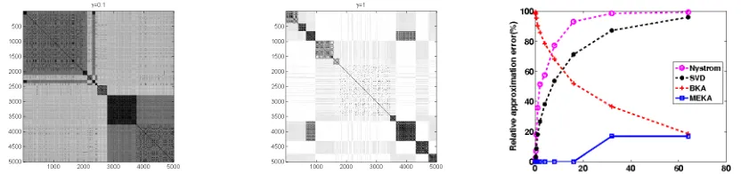
Let us examine two extreme cases of the Gaussian kernel: whenγ →0,G→eeT where e = [1, . . . ,1]T. As a consequence, G is close to low-rank when γ is small. However, at the other extreme as γ → ∞, G changes to the identity matrix, which has full rank with all eigenvalues equal to 1. In this case, G does not have a low-rank structure, but has a block/clustering structure. This observation motivates us to consider both low rank and clustering structure of the kernel matrix. Figures 1a and 1b give an example of the structure of a Gaussian kernel with differentγ on a real dataset by randomly sampling 5000 samples from the covtype dataset.
Before discussing further details, we first contrast the use of block and low-rank ap-proximations on the same dataset. We compare approximation errors for different methods when they use the same amount of memory in Figure 1c. Clearly, low-rank approximation methods work well only for very small γ values. Block Kernel Approximation (BKA), as proposed in Section 4.1, is a simple way to use clustering structure ofGthat is effective for large γ. Our proposed algorithm, MEKA, considers both block and low-rank structure of the kernel, and thus performs better than others under different γ values as seen in Figure 1c.
(a) The Gaussian kernel matrix withγ= 0.1 oncovtypedataset
(b) The Gaussian kernel matrix withγ= 1 oncovtypedataset
(c) Comparison of different kernel approximation methods for various γ.
Figure 1: (a) and (b) show that the structure of the Gaussian kernel matrix K(x,y) =
e−γkx−yk2 for the covtype data tends to become more block diagonal as γ increases(dark regions correspond to large values, while lighter regions correspond to smaller values). Plot (c) shows that low-rank approximations work only for small γ, and Block Kernel Approx-imation (BKA) works for large γ, while our proposed method MEKA works for small as well as largeγ.
4. Block Kernel Approximation
4.1 Clustering Structure of Shift-invariant Kernel Matrices
There has been substantial research on approximating shift-invariant kernels (Rahimi and Recht, 2007). A kernel functionK(xi,xj) is shift-invariant if the kernel value depends only on xi−xj, that is, K(xi,xj) = f(η(xi−xj)) where f(·) is a function that maps Rd to R, and η > 0 is a constant to determine the “scale” of the data. η is very crucial to the performance of kernel machines and is usually chosen by cross-validation. We further define
gu(t) =f(ηtu) to be a one variable function alongu’s direction whereuis an unit vector. We assume the kernel function satisfies the following property:
Assumption 1gu(t)is differentiable for all t6= 0.
Most of the practically used shift-invariant kernels satisfy the above assumption, for ex-ample, the Gaussian kernel (K(x,y) = e−γkx−yk22), and the Laplacian kernel (K(x,y) = e−γkx−yk1). It is clear that η2 is equivalent to γ for the Gaussian kernel if written in the form ofK(x,y) =f(η(x−y)). Whenη is large, off-diagonal blocks of shift-invariant kernel matrices will become small, and most of the information is concentrated in the diagonal blocks. To approximate the kernel matrix by exploiting this clustering structure, we first present a simple Block Kernel Approximation (BKA) as follows. Given a good partition V1, . . . ,Vc of the data points, where each Vs is a subset of {1, . . . , n}, BKA approximates the kernel matrix as:
G≈G˜ ≡
G(1,1) 0 . . . 0 0 G(2,2) . . . 0
..
. ... . .. ...
0 0 . . . G(c,c)
. (2)
Here,G(s,s)denotes the kernel matrix for blockVs – note that this implies that diagonal blocks ˜G(s,s)=G(s,s) and all the off-diagonal blocks, ˜G(s,t)= 0 withs6=t.
BKA is useful when ηis large. By analyzing its approximation error, we now show that k-means in the input space can be used to capture the clustering structure for shift-invariant kernels. The approximation error equalskG˜−Gk2
F =
P
i,jK(xi,xj)2−
Pc
s=1
P
i,j∈VsK(xi,xj) 2. Since the first term is fixed, minimizing the error kG˜−Gk2
F is the same with maximizing the second term, the sum of squared within-cluster entries D=Pc
s=1
P
i,j∈VsK(xi,xj) 2. However, directly maximizing D will not give a useful partition – the maximizer will assign all the data into one cluster. The same problem occurs in graph clustering (Shi and Malik, 2000; von Luxburg, 2007). A common approach is to normalize Dby each cluster’s size|Vs|. The resulting spectral clustering objective (also called ratio association) is:
Dkernel({Vs}cs=1) = c
X
s=1 1 |Vs|
X
i,j∈Vs
K(xi,xj)2. (3)
Theorem 1 For any shift-invariant kernel that satisfies Assumption 1,
Dkernel({Vs}c
s=1)≥C¯−η2R2Dkmeans({Vs}cs=1) (4)
where C¯ = nf(0)2 2, R is a constant depending on the kernel function, and Dkmeans ≡
Pc s=1
P
i∈Vskxi −msk 2
2 is the k-means objective function, where ms = (
P
i∈Vsxi)/|Vs|, s= 1,· · ·, c, are the cluster centers.
Proof We useu to denote the unit vector in the direction of xi−xj (xi 6=xj). By the mean value theorem, we have
K(xi,xj) =gu(ηkxi−xjk2) =gu(0) +ηg0u(s)kxi−xjk2 for somes∈(0, ηkxi−xjk2). By definition,f(0) =gu(0), so
f(0)≤K(xi,xj) +ηRkxi−xjk2, (5) whereR := sup
θ∈R,kvk=1
|gv0(θ)|. (6)
Squaring both sides of (5) we have
f(0)2 ≤K(xi,xj)2+η2R2kxi−xjk22+ 2K(xi,xj)(ηRkxi−xjk2).
From the classical arithmetic and geometric mean inequality, we can upper bound the last term by
2K(xi,xj)(ηRkxi−xjk2)≤K(xi,xj)2+η2R2kxi−xjk22,
therefore
f(0)2
2 ≤K(xi,xj)
2+η2R2kxi−xjk2
2. (7)
Plugging (7) into (3), we have
Dkernel({Vs}cs=1)≥ c
X
s=1 1 |Vs|
X
i,j∈Vs
f(0)2 2 −η
2R2kx
i−xjk22
≥ nf(0) 2 2 −η
2R2 c
X
s=1 1 |Vs|
X
i,j∈Vs
kxi−xjk22,
which can be manipulated to prove the desired bound (4).
(a)covtype (b)cadata
Figure 2: The Gaussian kernel approximation error of BKA using different ways to generate five partitions on 500 samples from covtype and cadata; on these data sets k-means in the input space performs similarly to spectral clustering on the kernel matrix, but is more efficient.
4.2 Speeding up Kernel SVM with BKA
In this section we will show how to use block kernel approximation(BKA) to divide kernel SVM problem into subproblems and significantly speed up the computation. Given a set of instance-label pairs (xi, yi), i= 1, . . . , n,xi∈Rdandy
i ∈ {1,−1}, the main task in training the kernel SVM is to solve the following quadratic optimization problem:
min
α f(α) = 1 2α
TQα−eTα, s.t. 0≤α≤C, (8)
whereeis the vector of all ones;C is the balancing parameter between loss and regulariza-tion in the SVM primal problem;α∈Rn is the vector of dual variables; andQis ann×n matrix withQij =yiyjGij, where Gij =K(xi,xj) is the kernel value betweeni-th andj-th sample. Lettingα∗ denote the optimal solution of (8), the decision value for a test data x can be computed by
n
X
i=1
α∗iyiK(x,xi). (9)
Due to high computation cost of directly solving kernel SVM, we can approximate the kernel matrix G by BKA to divide whole kernel SVM problem into subproblems, where each subproblem can be handled efficiently and independently.
To do this, we first partition the dual variables into k subsets {V1, . . . ,Vk}, where {V1, . . . ,Vk} are partitions generated by performing kmeans on the data points, and then solve the respective subproblems independently
min α(c)
1 2(α(c))
TQ
(c,c)α(c)−eTα(c), s.t. 0≤α(c)≤C, (10) where c= 1, . . . , k,α(c) denotes the subvector {αi |i∈ Vc} and Q(c,c) is the submatrix of
dataset Number of Number of d training samples testing samples
ijcnn1 49,990 91,701 22
census 159,619 39,904 409
covtype 464,810 116,202 54
Table 1: Dataset statistics
The quadratic programming problem (8) has n variables, and takes at least O(n2) time to solve in practice. By dividing it intok subproblems (10) with equal sizes, the time complexity for solving the subproblems can be reduced toO(k·(nk)2) =O(n2/k). Moreover, the space requirement is also reduced from O(n2) to O(n2/k2).
After computing all the subproblem solutions, we concatenate them to form an approxi-mate solution for the whole problem ¯α= [ ¯α(1), . . . ,α¯(k)], where ¯α(c)is the optimal solution for thec-th subproblem.
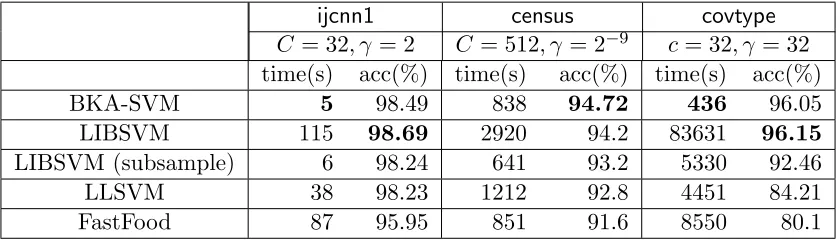
4.3 Comparing BKA-SVM with Low-rank Kernel SVM Solvers(BKA-SVM)
We now compare block structure based kernel SVM solver–BKA-SVM with low-rank struc-ture based kernel SVM solvers. All the experiments are conducted on an Intel 2.66GHz CPU with 8G RAM. We use 3 benchmark datasets as shown in Table 1. The thee datasets can be downloaded from http://www.csie.ntu.edu.tw/~cjlin/libsvmtools/datasets or the UCI data repository. We use a random 80%-20% split for covtype, and the original training/testing split for other datasets.
4.3.1 Competing Methods
We include the following exact kernel SVM solvers (LIBSVM), approximate low-rank SVM solvers (LLSVM, FastFood) in our comparison:
1. LIBSVM: the implementation in the LIBSVM library (Chang and Lin, 2011) with a small modification to handle SVM without the bias term – we observe that LIBSVM has similar test accuracy with/without bias. We also include the results for using LIBSVM with random 1/5 subsamples on each dataset in Table 2.
2. LLSVM: improved Nystr¨om method for nonlinear SVM by (Wang et al., 2011). We solve the resulting linear SVM problem by the dual coordinate descent solver in LIB-LINEAR (Hsieh et al., 2008).
3. FastFood: use random Fourier features to approximate the kernel function (Le et al., 2013). We solve the resulting linear SVM problem by the dual coordinate descent solver inLIBLINEAR.
ijcnn1 census covtype
C = 32, γ = 2 C = 512, γ = 2−9 c= 32, γ= 32 time(s) acc(%) time(s) acc(%) time(s) acc(%)
BKA-SVM 5 98.49 838 94.72 436 96.05
LIBSVM 115 98.69 2920 94.2 83631 96.15
LIBSVM (subsample) 6 98.24 641 93.2 5330 92.46
LLSVM 38 98.23 1212 92.8 4451 84.21
FastFood 87 95.95 851 91.6 8550 80.1
Table 2: Comparison on real datasets using the RBF kernel.
4.3.2 Parameter Setting
We consider the RBF kernel K(xi,xj) = exp(−γkxi−xjk2
2). We use same kernel func-tion for both training and test phases. We chose the balancing parameter C and kernel parameter γ by 5-fold cross validation on a grid of points: C = [2−10,2−9, . . . ,210] and
γ = [2−10, . . . ,210] for ijcnn1, census, and covtype. For BKA-SVM, we set the number of clusters to be 64 for these three datasets. There is a tradeoff between the number of clus-ters and prediction accuracy. If we increase the number of clusclus-ters, BKA-SVM will become faster, but the prediction accuracy will mostly decrease. On the other hand, if the number of clusters is set smaller, BKA-SVM can achieve higher accuracy (in most cases), while takes more time to train. The following are parameter settings for other methods in Table 2: the rank is set to be 3000 in LLSVM; number of Fourier features is 3000 in Fastfood1; the tolerance in the stopping condition for LIBSVM is set to 10−3 (the default setting of
LIBSVM).
Tables 2 present time taken and test accuracies. Experimental results show that the BKA-SVM achieves near-optimal test performance. Also we observe that BKA-SVM per-forms better than low-rank approximation based methods for kernel SVM problem showing the benefit of using block structure of kernel matrix.
We can see that BKA exploits the block structure of kernel matrix, and can speed up the training of kernel SVM. As shown in Tandon et al. (2016), BKA can also be used for speeding up kernel ridge regression problem. About the memory requirement, which is the main theme of this paper, BKA takes O(nk2) memory to approximate the kernel matrix, while popular low-rank based kernel approximation methods are more memory efficient, and only need linear memory to represent the kernel matrix.
5. Memory Efficient Kernel Approximation
There are two main drawbacks of the BKA approach: (i) it ignores all off-diagonal blocks, which results in large error whenη is small (as seen in Figure 1(c)); (ii) for large-scale kernel approximation, it is too expensive to compute and store all the diagonal block entries. To
overcome these two drawbacks, we propose to use low-rank representation for each block in the kernel matrix.
5.1 Low Rank Structure of Each Block
To motivate the use of low-rank representation in our proposed method, we first present the following bound:
Theorem 2 Given data pointsx1, . . . ,xn ∈Rd, and a partition V1, . . . ,Vc, and assume f
is Lipschitz continuous, then for any s, t (s=t or s6=t)
kG(s,t)−G(s,t)k kF≤4Ck−1/d
p
|Vs||Vt|min(rs, rt),
where G(s,t)k is the best rank-k approximation to G(s,t); C is the Lipschitz constant of the shift-invariant function f; rs is the radius of the s-th cluster.
Proof To prove this theorem, we use the -net theorem in (Cucker and Smale, 2001), which states that when all the data xi∈Rd,i= 1,· · · , nare in a ball with radius r, there exist T = (4r¯r)d balls of radius ¯r that cover all the data points. If we set T to bek, then ¯
r=k−1/d4r.
Let x1, . . . ,xns be the data points in the s-th cluster, and let y1, . . . ,ynt be the data points in the t-th cluster, and ns = |Vs|, nt = |Vt|. Our goal is to show that G(s,t) is low-rank, whereG(s,t)i,j =K(xi,yj). Assumertis the radius of thet-th cluster, therefore we can find kballs with radius ¯r=k−1/d4rt to cover{yj}nj=1t .
Assume centers of the balls for t-th cluster are m1,m2, . . . ,mk, then we can form a low-rank matrix ¯G(s,t) = ¯UV¯T, where for alli= 1, . . . , ns, j = 1, . . . , nt, and q= 1, . . . , k,
¯
Ui,q=K(xi,mq) and ¯Vj,q =
(
1 ifyj ∈Ball(mq),
0 otherwise.
Assume yj is in ballq, then
(G(s,t)ij −G¯(s,t)ij )2= (f(xi−yj)−f(xi−mq))2 ≤C2k(xi−yj)−(xi−mq)k2 =C2kyj−mqk22
≤C2¯r2.
Therefore, if (G(s,t))∗ is the best rank-kapproximation for G(s,t), then kG(s,t)−(G(s,t))∗kF ≤ kG(s,t)−G¯(s,t)kF ≤Ck−1/d4rt
√
nsnt. (11)
Similarly, by coverings-th cluster{xi}ns
i=1 withkballs we can get the following inequality:
kG(s,t)−(G(s,t))∗kF ≤Ck−1/d4rs √
nsnt. (12)
16 14 13 7 7
14 29 13 9 9
13 13 20 10 10
7 9 10 29 11
7 9 10 11 28
(a) k-means clustering.
139 99 101 44 45 99 116 86 43 44 101 86 131 46 47
44 43 46 47 45
45 44 47 45 49
(b) a random partition.
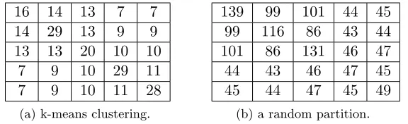
Table 3: Rank of each of the 5 blocks (from a subsampled ijcnn1 data set) using different partition strategies: (a) by k-means clustering; (b) by a random partition.
Theorem 2 suggests that each block(diagonal or off-diagonal block) of the kernel matrix will be low-rank if we find the partition by k-means in the input space and the radius of the cluster is small. In the following we present empirical confirmation of this result. In Table 3, we present the numerical rank of each block, where numerical rank for am by nmatrix
A is defined as the number of singular values with magnitude larger than max(n, m)kAk2δ whereδ is a small tolerance 10−6. We sample 4000 data points from theijcnn1dataset and generate 5 clusters by k-means and random partition. Table 3a shows the numerical rank for each block using k-means, while Table 3b shows the numerical rank for each block when the partitions are random. We observe that by using k-means, the rank of each block is fairly small.
5.2 Memory Efficient Kernel Approximation (MEKA)
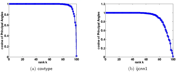
Based on the above observation, we propose a fast and memory efficient scheme to approx-imate shift-invariant kernel matrices. As suggested by Theorem 2, each block tends to be low-rank after k-means clustering; thus we can form a rank-k approximation for each of thec2 blocks separately to achieve low error; however, this approach would requireO(cnk) memory, which can be prohibitive. Therefore, our proposed method first performs k-means clustering, and after rearranging the matrix according to clusters, it computes the low-rank basis only for diagonal blocks (which are more dominant than off-diagonal blocks) and uses them to approximate off-diagonal blocks. Empirically, we observe that the principal angles between the dominant singular subspaces of diagonal block and off-diagonal block are small (as shown in Figure 3). In Figure 3, we randomly sampled 1000 data points from the cov-type and ijcnn1 datasets and generated 5 clusters by k-means for each dataset. The blue line shows the cosines of the principal angles between the dominant singular subspace of a diagonal block G(s,s) and that of an off-diagonal block G(s,t) for different ranksk, where s
andtare randomly chosen. We can observe that most of the cosines are close to 1, showing that there is substantial overlap between the dominant singular subspaces of the diagonal and off-diagonal block.
(a)covtype (b)ijcnn1
Figure 3: The cosines of the principal angles between the dominant singular subspaces of diagonal block and off-diagonal block of a Gaussian kernel ((a): γ = 0.1 and 1000 random samples from covtype; (b): γ = 1 and 1000 random samples from ijcnn1) with respect to different ranks. The cosines of the principal angles are close to 1 showing that two subspaces are similar.
W(s)L(s,s)(W(s))T, we form the following memory-efficient kernel approximation: ˜
G=W LWT, (13)
whereW is a diagonal matrix as
W ≡
W(1) 0 . . . 0
0 W(2) . . . 0 ..
. ... . .. ...
0 0 . . . W(c)
; (14)
andLis a “link” matrix consisting ofc2 blocks, where eachk
s×ktblockL(s,t)captures the interaction between thesth andtth clusters. For now, let us first assume ks=k ∀s(we will discuss different strategies to choose ks later). Note that if we were to restrict L to be a block diagonal matrix, ˜Gwould still be a block diagonal approximation ofG. However, we consider the more general case that L is dense. In this case, each off-diagonal block G(s,t)
is approximated as W(s)L(s,t)(W(t))T, and this approximation is memory efficient as only
O(k2) additional memory is required to represent the (s, t) off-diagonal block. If a rank-k
approximation is used within each cluster, then the generated approximation has rankck, but only needs a total of O(nk+ (ck)2) storage.
Computing W(s). Since we aim to deal with dense kernel matrices of huge size, we use the standard Nystr¨om approximation to compute low-rank “basis” for each diagonal block. When applying the standard Nystr¨om method to ans×ns block G(s,s), we sample
m columns from G(s,s), evaluate their kernel values, compute the rank-k pseudo-inverse of an m×m matrix, and form G(s,s) ≈ W(s)L(s,s)(W(s))T. The time required per block is
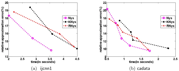
in Section 2. In Figure 4 we compare using standard Nystr¨om(Nys)(Williams and Seeger, 2001), k-means Nystr¨om(KNys)(Zhang and Kwok, 2010), and Nystr¨om with randomized SVD(RNys)(Li, Kwok, and Lu, 2010) to generateW(s) on bothijcnn1and cadatadatasets. As shown in Figure 4, we observe that the standard Nystr¨om method combined with MEKA gives excellent performance.
(a) ijcnn1 (b)cadata
Figure 4: Comparison of using Nys, KNys, and RNys to obtain the basisW(s) for diagonal blocks in MEKA on ijcnn1 and cadata datasets. The x-axis shows the computation time and y-axis shows the relative kernel approximation error(%).
Computing L(s,t). The optimal least squares solution forL(s,t)(s6=t) is the minimizer of the local approximation errorkG(s,t)−W(s)L(s,t)(W(t))Tk
F. However, forming the entire
G(s,t) block can be time consuming. For example, computing the whole kernel matrix for
mnist2m with 2 million data points takes more than a week. Therefore, to compute L(s,t), we propose to randomly sample a (1 +ρ)k×(1 +ρ)ksubmatrix ˆG(s,t)from G(s,t), and then find L(s,t) that minimizes the error on this submatrix. If the row/column index set for the subsampled submatrix ˆG(s,t) inG(s,t) is vs/vt, thenL(s,t) can be computed in closed form:
L(s,t)= ((Wv(s)s )TWv(s)s )−1(Wv(s)s )TGˆ(s,t)Wv(t)t ((Wv(t)t )TWv(t)t )−1,
whereWv(s)s and W (t)
vt are formed by the rows inW(s) and W(t) with row index sets vs and vt respectively.
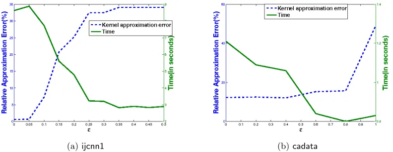
Since there are only k2 variables in L(s,t), we do not need too many samples for each block, and the time to compute L(s,t) is O((1 +ρ)3k3). In practice, we observe that set-ting ρ to be 2 or 3 is enough for a good approximation, so the time complexity is O(k3). Empirically, many values in the off-diagonal blocks are close to zero, and only a few of them have large values as shown in Figure 1. Based on this observation, we further propose a thresholding technique to reduce the time for storing and computing L(s,t). Since the distance between cluster centers is a good indicator for the values in an off-diagonal block, we can set the whole block L(s,t) to 0 if K(ms,mt) ≤ for some thresholding parameter
of thresholding parameter on the ijcnn1 and cadata data in Figure 5. When is large, although MEKA yields higher approximation error(because it omits more off-diagonal in-formation), it is faster. On the other hand, for small, when more off-diagonal information is considered, we notice an increase in time and smaller in approximation error. In practice, we need to use cross-validation to select.
(a)ijcnn1 (b)cadata
Figure 5: Time (in seconds) and kernel approximation quality of MEKA when varying the thresholding parameterfor setting off-diagonal blocks inL to be zero.
Choosing the rank ks for each cluster. We need to decide the rank for the
sth(s= 1,· · ·, c) cluster,ks, which can be done in different ways: (i) the samek for all the clusters; (ii)ksis proportional to the size ofsthcluster; (iii) eigenvalues based approach. For (iii), supposeM(s)is thems×msmatrix consisting of the intersection ofmssampled columns inG(s,s), andMis thecm×cm(Pc
s=1ms =cm) block-diagonal matrix withM(s)as diagonal block. We can choosekssuch that the set of top-ckeigenvalues ofMis the union of the eigen-values ofM(s)in each cluster, that is, [σ1(M), . . . , σck(M)] =∪cs=1[σ1(M(s)), . . . , σks(M
(s))]. To use (iii), we can oversample points in each cluster, e.g., sample 2k points from each cluster, perform eigendecompostion of a 2k×2k kernel matrix, sort the eigenvalues from
c clusters, and finally select the top-ck eigenvalues and their corresponding eigenvectors. Comparing these three strategies, (i) achieves lower memory usage and is fastest, and (ii) is more accurate than (i) with more memory usage, while (iii) is slowest but achieves lower error for diagonal blocks. In Figure 6, we compare these three sampling strategies to choose
ks on ijcnn1 and cadata datasets. It is shown that these three methods perform similarly well and choosing ks to be same for each cluster performs sightly better than by the size of each cluster and singular values based approach. In the experiment, we set all the clus-ters to have the same rank k. We show that this simple choice of ks already outperforms state-of-the-art kernel approximation methods.
(a)ijcnn1 (b)cadata
Figure 6: Comparison of different strategies to choose the rankks of each cluster in MEKA on ijcnn1and cadatadatasets.
Method Storage Rank Time Complexity
RKS (Rahimi and Recht, 2008) O(cnk) ck O(cnkd)
Nystr¨om(Williams and Seeger, 2001) O(cnk) ck O(cnm(ck+d) + (cm)3)
SVD O(cnk) ck O(n3+n2d)
MEKA O(nk+ (ck)2) ck O(nm(k+d) +cm3+TL+TC)
Table 4: Memory and time analysis of various kernel approximation methods, whereTL is the time to compute the matrixL and TC is the time for clustering in MEKA.
meansTL can at most be O(12c2k3); (2)TC is proportional to the number of samples. For a large dataset, we sample 20000 points for k-means, and thus the clustering is more efficient than working on the entire data set.
Algorithm 1 Memory Efficient Kernel Approximation (MEKA) Input : Data points{(xi)}n
i=1, scaling parameterγ, rank k, and no. of clusters c. Output: The rank-ck approximation ˜G=W LWT using O(nk+ (ck)2) space Generate the partition V1, . . . ,Vc by k-means;
for s= 1, . . . , c do
Perform the rank-kapproximation G(s,s)≈W(s)L(s,s)(W(s))T by standard Nystr¨om;
end
forall(s, t)(s6=t) do
Sample a submatrix ¯G(s,t) fromG(s,t) with row index set vs and column index setvt;
FormWv(s)s by selecting the rows inW
(s) according to index setvs; FormWv(t)t by selecting the rows in W(t) according to index setvt; Solve the least squares problem: ¯G(s,t)≈Wv(s)s L
(s,t)(W(t) vt )
Dataset TC TW TL
pendigit 0.05 0.69 0.35
ijcnn1 0.15 1.27 0.84
covtype 1.83 9.82 12.23
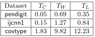
Table 5: Time (in seconds) for each step of MEKA, where TW is the time to compute low-rank approximation for the diagonal block matrices; TL is the time to form the “link” matrixL;TC is the time for performing k-means clustering.
In Table 5, we show the time cost for each step of MEKA on pendigit, ijcnn1, and
covtype datasets. The execution time of our proposed algorithm mainly consists of three parts:(1) time for performing k-means clustering (TC), (2) time for forming the “basis” W
from the diagonal blocks (TW), (3) time to compute the link matrix L from off-diagonal blocks (TL). From Table 5, we observe that compared with TW and TL, TC is fairly small and TW dominates the whole process in most cases. For covtype data set, since we choose
c to be large,TL is sightly larger thanTW. We will analyzeTW,TL, and TC for different c in the experiment part.
5.3 Analysis
We now bound the approximation error for our proposed method. We show that when
σk+1−σck+1 is large, whereσk+1 andσck+1 are thek+ 1st andck+ 1st singular values ofG respectively, and entries in off-diagonal blocks are small, MEKA has a better approximation error bound compared to standard Nystr¨om that uses similar storage.
Theorem 3 Let ∆ denote a matrix consisting of all off-diagonal blocks of G, so ∆(s,t) =
G(s,t) for s6=t and all zeros when s=t. We sample cm points from the dataset uniformly at random without replacement and split them according to the partition from k-means, such that each cluster has ms benchmark points and Pcs=1ms = cm. Let Gck be the best
rank-ckapproximation ofG, and G˜ be the rank-ck approximation from MEKA. Suppose we choose the rankks for each diagonal block using the eigenvalue based approach as mentioned
in Section 5.1, then with probability at least 1−δ, the following inequalities hold for any sample of sizecm:
kG−G˜k2≤ kG−Gckk2+ 1 √
c
2n
√
mGmax(1 +θ) + 2k∆k2,
kG−G˜kF≤ kG−GckkF+
64k m
14
nGmax(1+θ)
1
2+2k∆kF
where θ = qnn−−0.5m β(m,n)1 log1δdGmax/G 1 2
max; β(m, n) = 1− 2 max{m,n1 −m};Gmax = maxiGii;
and dGmax represents the distance maxijp
Proof Let B denote the matrix formed by the diagonal block of G, that is, B≡
G(1) 0 . . . 0 0 G(2) . . . 0
..
. ... . .. ... 0 0 . . . G(c)
. (15)
According to the definition of ∆, G= B+ ∆. In MEKA, the error kG˜ −Gk2 consists of two components,
kG˜−Gk2 =kB˜−B+ ( ˜∆−∆)k2 ≤ kB˜−Bk2+k∆˜ −∆k2 (16) where ˜B and ˜∆ are the approximations forB and ∆ in MEKA respectively.
Let us first consider the error in approximating the diagonal blocks kB˜−Bk2. Since we sample cm benchmark points from n data points uniformly at random without re-placement and distribute them according to the partition coming from k-means, the s -th cluster now has ms benchmark points with Ps=cs=1ms = cm. For the s-th diagonal blockG(s), we will perform the rank-ksapproximation using standard Nystr¨om, so we have
G(s)≈E(s)(Mk(s)s )+E(s), whereE(s)denotes the matrix formed bymssampled columns from
G(s) and M(s)
ks is ams×ms matrix consisting of the intersection of sampled ms columns. Suppose we use the singular value based approach to choose ks for s-th cluster as de-scribed in Section 5.1, and
Mck+equiv
(Mk(1) 1 )
+ 0 . . . 0
0 (Mk(2) 2 )
+ . . . 0
..
. ... . .. ...
0 0 . . . (Mk(c)
c ) +, (17)
where M is the cm ×cm block diagonal matrix that consists of the intersection of the sampled cmcolumns. Then we can see that approximating the diagonal blocks B is equiv-alent to directly performing standard Nystr¨om on B by sampling cm benchmark points uniformly at random without replacement to achieve the rank-ckapproximation. The stan-dard Nystr¨om’s norm-2 and Frobenius error bound are given in (Kumar et al., 2009), so kB−B˜k2 can be bounded with probability at least 1−δ as
kB−B˜k2 ≤ kB−Bckk2+ 2n
√
cmBmax[1 +
s
n−cm n−0.5
1
β(cm, n)log 1 δd B max/B 1 2
max], whereBck denotes the best rank-ckapproximation to B;Bmax= maxiBii;dBmaxrepresents the distance maxijpBii+Bjj−2Bij.
To bound k∆˜ −∆k2, recall that some off-diagonal blocks in MEKA are set to 0 by thresholding and 0 is one special solution of least squares problem to compute L(s,t), we have k∆˜ −∆k2 ≤ k∆k2.
Furthermore, according to perturbation theory (Stewart and Ji-Guang, 1990), we have
The inequality in (16) combined with (18) gives a bound onkG˜−Gk2 as,
kG˜−Gk2≤ kB−Bckk2+k∆k2+ 2n
√
cmBmax[1 +
s
n−cm n−0.5
1
β(cm, n)log 1 δd B max/B 1 2 max]
≤ kG−Gckk2+ 2k∆k2+ 2n
√
cmBmax[1 +
s
n−cm n−0.5
1
β(cm, n)log 1 δd B max/B 1 2 max]
≤ kG−Gckk2+ 2k∆k2+ 2n
√
cmGmax[1 +
s
n−cm n−0.5
1
β(cm, n)log 1 δd G max/G 1 2 max]
≤ kG−Gckk2+ 2k∆k2+ 1 √
c
2n
√
mGmax[1 +
s
n−m n−0.5
1
β(m, n)log 1 δd G max/G 1 2 max],
whereGck denotes the best rank-ckapproximation toG;Gmax= maxiGii;dGmaxrepresents the distance maxij
p
Gii+Gjj−2Gij. The third inequality is becauseG=B+ ∆,Bmax≤
Gmax and dBmax≤dmaxG . The last inequality is because nm andncm.
Similarly by using perturbation theory and upper bounds for the Frobenius error of standard Nystr¨om, the result follows.
When ks(s= 1,· · · , c) is balanced (meaningks is approximately the same for each clus-ter) andnis large, MEKA provides a rank-ckapproximation using roughly the same amount of storage as rank-k approximation by standard Nystr¨om. Interestingly, from Theorem 3, ifkG−Gkk2− kG−Gckk2 ≥2k∆k2, then
kG−G˜k2≤ kG−Gkk2+ 1 √
c
2n
√
mGmax(1 +θ).
The second term in the right hand side of above inequality is only √1
c of that in the spectral norm error bound for standard Nystr¨om that uniformly samplesmcolumns without replace-ment inGto obtain the rank-kapproximation as shown in (Kumar, Mohri, and Talwalkar, 2009). Thus, if there is a large enough gap betweenσk+1 andσck+1, the error bound for our proposed method is better than standard Nystr¨om that uses similar storage. Furthermore, when γ is large,Gtends to have better clustering structure, suggesting in Theorem 3 that k∆k is usually quite small. Note that when using the same rank kfor all the clusters, the above bound can be worse because of some extreme cases, e.g., all the top-ck eigenvalues are in the same cluster. In practice we do not observe those extreme situations. We also want to mention that bothk∆kF and k∆k2 will be affected by the number of clustersc.
6. Experimental Results
Dataset n d Dataset n d wine 6,497 11 census 22,784 137
cpusmall 8,192 12 ijcnn1 49,990 22
pendigit 10,992 16 covtype 581,012 54
cadata 20,640 8 mnist2m 2,000,000 784
Table 6: Data set statistics (n: number of samples;d: dimension of samples).
the Gaussian kernel, but we observe similar behavior on other shift-invariant kernels (see Section 6.2). Note that the same kernel function is used in both training and test phases. We compare our method with six state-of-the-art kernel approximation methods:
1. The standard Nystr¨om method (denoted by Nys)(Williams and Seeger, 2001). In the experiment, we uniformly sample 2kcolumns of Gwithout replacement, and run Nystr¨om for rank-k approximation.
2. Kmeans Nystr¨om (denoted by KNys)(Zhang and Kwok, 2010), where the landmark points are the cluster centroids. As suggested in (Zhang et al., 2012), we sample 20000 points for clustering when the total number of data samples is larger than 20000.
3. Random Kitchen Sinks (denoted by RKS)(Rahimi and Recht, 2008), which approxi-mates the shift-invariant kernel based on its Fourier transform.
4. Fastfood with “Hadamard features” (denoted by fastfood)(Le, Sarlos, and Smola, 2013).
5. Ensemble Nystr¨om (denoted by ENys) (Kumar, Mohri, and Talwalkar, 2009). Due to concern for the computation cost, we set the number of “experts” in ENys 3.
6. Nystr¨om using randomized SVD (denoted by RNys)(Li, Kwok, and Lu, 2010). We set the number of power iterations q= 1 and oversampling parameter p= 10.
We compare all the methods on two different tasks: kernel low-rank approximation and kernel ridge regression. We do not compare with BKA in this section, because (1) the approximation error of BKA is large whenγis small (as shown in Figure 1); (2) BKA is time consuming because it needs to compute all the diagonal blocks’ kernel values, which needs
O(n2cd) time; (3) BKA is not memory efficient to approximate the kernel matrix, because it needs O(nc2) space to store the approximation. All the experiments are conducted on a machine with an Intel Xeon X5440 2.83GHz CPU and 32G RAM.
6.1 Kernel Approximation Quality
We now compare the kernel approximation quality for the above methods.
Main results. The kernel approximation results are shown in Figure 7 and Table 7. We use relative kernel approximation error kG−G˜kF/kGkF to measure the quality. We randomly sampled 20000 rows of G to evaluate the relative approximation error for
Dataset k γ c Nys RNys KNys ENys RKS fastfood MEKA
pendigit 128 2 5 0.1325 0.1361 0.0828 0.2881 0.4404 0.4726 0.0811
ijcnn1 128 1 10 0.0423 0.0385 0.0234 0.1113 0.2972 0.2975 0.0082
covtype 256 10 15 0.3700 0.3738 0.2752 0.5646 0.8825 0.8920 0.1192
Table 7: Comparison of approximation error of our proposed method with six other state-of-the-art kernel approximation methods on real datasets, where γ is the Gaussian scaling parameter; c is the number of clusters in MEKA; k is the rank of each diagonal-block in MEKA and the rank of the approximation for six other methods. Note that for a given
k, every method has roughly the same amount of memory. All results show relative kernel approximation errors for each k.
and from 20 to 200 for the pendigitdata. Figure 7 shows that our proposed approximation scheme always achieves lower error with less time and memory. The main reason is that using similar amount of time and memory, our method aims to approximate the kernel matrix by a rank-ckapproximation, while all other methods are only able to form a rank-k
approximation.
In Table 7, we fix the rank k and γ, so that each method has the same memory usage of low-rank representation, and compare MEKA with them in terms of relative approxima-tion error. As it can be seen, under the same amount of memory, our proposed method consistently yields lower approximation error than other methods.
Also as we can see from Table 7 and Figure 8, Nystr¨om based methods perform much better than random features based methods (including RKS and Fastfood here) in terms of kernel approximation quality. Therefore we do not show their performance in Figure 7, so that we could see the difference between MEKA and other Nystr¨om based methods.
Robustness to the Gaussian scaling parameter γ. To show the robustness of our proposed algorithm with differentγ as explained in Section 3, we test its performance on the ijcnn1 (Figure 9a), cadata (Figure 9b) and sampled covtype datasets (Figure 1c). The relative approximation errors for different γ values are shown in the figures using a fixed amount of memory. For large γ, the kernel matrix tends to have a block structure, so our proposed method yields lower error than other methods. The gap becomes larger as γ increases. Interestingly, Figure 1c shows that the approximation error of MEKA is superior to even the exact SVD, as it is much more memory efficient. Even for small γ
where the kernel exhibits low-rank structure, our proposed method performs better than Nystr¨om based methods, suggesting that it can get the low-rank structure of the kernel matrix.
(a) pendigit (γ = 2), memory vs approx. error.
(b)ijcnn1(γ= 1), memory vs ap-prox. error.
(c) covtype (γ = 1), memory vs approx. error.
(d) pendigit (γ = 2), time vs ap-proximation error.
(e)ijcnn1(γ= 1), time vs approx-imation error.
(f) covtype (γ = 1), time vs ap-proximation error.
(g)pendigit (γ = 10), memory vs approximation error.
(h)ijcnn1(γ= 10), memory vs ap-proximation error.
(i) covtype (γ = 10), memory vs approximation error.
(j)pendigit (γ = 10), time vs ap-proximation error.
(k) ijcnn1 (γ = 10), time vs ap-proximation error.
(l) covtype (γ = 10), time vs ap-proximation error.
Figure 8: Comparison between Nystr¨om based methods (MEKA and standard Nystr¨om) and random feature based methods (RKS and fastfood). We can see that Nystr¨om based methods perform much better than random feature based methods for kernel approximation.
(a)ijcnn1. (b)cadata.
Figure 9: The kernel approximation errors for different Gaussian scaling parameter γ.
ijcnn1dataset when varying the number of clusters c. Here the parameter γ is set to be 1. From Figure 10b, we observe that when the number of clusterscis small,TW will dominate the whole process. As cincreases, the time for computing the link matrix L,TL, increases. This is because the number of off-diagonal blocks increases quadratically with c. Since the time complexity for k-means is O(ncd),TC increases linearly withc.
6.2 The Performance of MEKA for Approximating the Laplacian Kernel
(a) kernel approximation under different num-bers of clusters c in MEKA. For standard Nystr¨om(Nys), Randomized Nystr¨om(RNys), and Kmeans Nystr¨om(KNys), we use the same memory with MEKA.
(b) Time for each step of MEKA when varying the number of clustersc. TC is the time for
perform-ing k-means clusterperform-ing; TW is the time to form
the “basis”W from the diagonal blocks; andTL
is the time to computeLfrom off-diagonal blocks.
Figure 10: The kernel approximation errors and time cost for each step of MEKA when varyingc onijcnn1 dataset.
(a) memory vs approximation error. (b) time vs approximation error.
Figure 11: Low-rank Laplacian kernel approximation results forijcnn1dataset.
6.3 Kernel Ridge Regression
Next we compare the performance of various methods on kernel ridge regression (Saunders, Gammerman, and Vovk, 1998):
max α λα
Tα+αTGα−2αTy, (19)
where Gis the kernel matrix formed by training samples {x1, . . . ,xl}, andy∈Rl are the targets. For each kernel approximation method, we first form the approximated kernel ˜G, and then solve (19) by conjugate gradient (CG). The main computation in CG is the matrix vector product ˜Gv. Using low-rank approximation, this can be computed usingO(nk) flops. For our proposed method, we compute W LWTv, where WTv = Pc
Dataset k γ c λ Nys RNys KNys ENys RKS fastfood MEKA wine 128 2−10 3 2−4 0.7514 0.7555 0.7568 0.7732 0.7459 0.7509 0.7375
cadata 128 22 5 2−3 0.1504 0.1505 0.1386 0.1462 0.1334 0.1502 0.1209 cpusmall 256 22 5 2−4 8.8747 8.6973 6.9638 9.2831 9.6795 10.2601 6.1130 census 256 2−4 5 2−5 0.0679 0.0653 0.0578 0.0697 0.0727 0.0732 0.0490 covtype 256 22 10 2−2 0.8197 0.8216 0.8172 0.8454 0.8011 0.8026 0.7106
mnist2m 256 2−5 40 2−5 0.2985 0.2962 0.2725 0.3018 0.3834 na 0.2667
Table 8: Comparison of our proposed method with six other state-of-the-art kernel approx-imation methods on real datasets for kernel ridge regression, where λ is the regularization constant. All the parameters are chosen by cross validation, and every method has roughly the same amount of memory as in Table 7. All results show test RMSE for regression for each k. Note that k for fastfood needs to be larger than d, so we cannot test fastfood on
mnist2mwhen k= 256.
O(nk) flops,L(Wv) requiresO(kLk0) flops, andW(LWTv) requiresO(nk) flops. Therefore, the time complexity for computing the matrix vector product for both MEKA and low-rank approximation methods is proportional to the memory for storing the approximate kernel matrices. Besides kernel approximation algorithms, we compare our method with another divide-and-conquer based kernel ridge regression method (denoted DC-KRR)(Zhang et al., 2013). The basic idea in Zhang et al. (2013) is to randomly partition the data into c parts and then train a kernel ridge regression model in each partition. To test a new data point, it will be tested on each submodel and the final prediction is the average ofc predictions.
The parameters are chosen by five fold cross-validation and shown in Table 8. The rank for these algorithms is varied from 100 to 1000. The test root mean square error (test RMSE) is defined as kyte −Gteαk, where yte ∈ Ru is testing labels and Gte ∈
Ru×l is the approximate kernel values between testing and training data. Thecovtypeandmnist2m
data sets are not originally designed for regression, and here we set the target variables to be 0 and 1 formnist2mand -1 and 1 forcovtype. Table 8 compares the kernel ridge regression performance of our proposed scheme with six other methods given the same amount of memory or samekin terms of test RMSE. It shows that our proposed method consistently performs better than other methods. Figure 12 shows the time usage of different methods for regression by varying the memory or rankk. As we can see that using the same amount of time, our proposed algorithm always achieves the lowest test RMSE. The total running time consists of the time for obtaining the low-rank approximation and time for regression. The former depends on the time complexity for each method, and the latter depends on the memory requirement to store the low-rank matrices. As shown in the previous experiment, MEKA is faster than the other methods while achieving lower approximation error and using less memory. As a consequence, it achieves lower test RMSE in less time compared to other kernel approximation methods.
7. Conclusions and Discussions
(a)wine, time vs regression error. (b)cpusmall, time vs regression er-ror.
(c) cadata, time vs regression er-ror.
(d) census, time vs regression er-ror.
(e)covtype, time vs regression er-ror.
(f)mnist2m, time vs regression er-ror.
Figure 12: Kernel ridge regression results for various data sets. Methods with regression error above the top ofy-axis are not shown. All results are averaged over five independent runs.
parameter is changed. Our method exploits both low-rank and block structure present in the kernel matrix, and thus performs better than previously proposed low-rank based methods in terms of approximation and regression error, speed and memory usage. The code for MEKA is available at www.cs.utexas.edu/~ssi/meka/. We will discuss next about some typical problems encountered when using MEKA and how to deal with them.
7.1 Dealing with the Non-PSD Issue
If for each off-diagonal block, we sample all the entries, the resulting approximate matrix in MEKA will be positive semidefinite(PSD). The reason is as follow: if we use all the all-diagonal blocks to compute the link matrix L, the approximation will be G≈ W LWT
withL=WTGW. Since Gis PSD, so it is with L, which provesW LWT will be PSD. However, due to the sampling procedure in MEKA, the resulting approximate matrix might not be PSD, which will cause some problems when PSD is required for some ap-plications, e.g., kernel SVM with hinge loss. There are two simple and effective ways to solve this issue: (1) The first method (MEKA-PSD) is to set negative eigenvalues to 0. The procedure is first to perform eigen-decomposition on the small ck×ck ”link” matrix
L=U SUT(whereU and S are the eigenvector and eigenvalue matrices forL respectively) in the MEKA representation, and then shrink its negative eigenvalues to be 0, which forms the new eigenvalue matrix ¯SforL. After that, the new MEKA approximation will become:
¯
shrinking operation, both the kernel approximation error and computation time will in-crease slightly. We show the comparison of Nys, MEKA and MEKA-PSD onijcnn1dataset in Figure 13. We can see that to achieve similar approximation, MEKA-PSD is slightly slower than MEKA, but still performs better than Nys, which also generates PSD kernel approximation. (2) The second method is to directly add a small valueto the diagonal of
¯
G, which is equivalent to using regularization term when applying MEKA for kernel meth-ods. We show the kernel ridge regression results in Table 8, where we add regularization term to MEKA. Note that to make sure the resulting MEKA approximation is PSD for the second method,should be equal or larger than the absolute value of the smallest negative eigenvalue of ¯G.
Figure 13: MEKA-PSD kernel approximation results forijcnn1dataset.
7.2 Dealing with the Instability Issue
There are two steps in Algorithm 1 that might cause the approximation unstable. One is due to the basis formed from each diagonal block–Wi. If the kernel matrix has strong block-diagonal structure, choosing columns from block-diagonal blocks to formW will perform well; on the contrary, if the kernel matrix does not have very strong block structure, other sampling strategies can be involved, for example, sampling columns from the rows corresponding to each partition to form the basis. Another step which might cause unstable result is due to insufficient entries sampled when forming the ”link” matrix L. One way to solve this issue is to sample more entries from each off-diagonal block to form L when the computation time is not the main concern.
7.3 Other Applications using MEKA
In the experiment section, we apply MEKA for kernel approximation and kernel ridge regression, and besides that we could use our MEKA framework for many other machine learning applications: such as speeding up the computation of the inverse of the kernel matrix.
G≈W LWT, the inverse operation can be done in a faster fashion using Woodbury formula.
(λI+G)−1 ≈(λI+W LWT)−1 = 1
λ(I −W(λL
−1+WTW)−1WT)
We can see that after the approximation, we only need to inverse theck×ckmatrix which reduce the time complexity for inverse of the dense matrix fromO(n3) toO(n(ck)2+ (ck)3). Besides speeding up the matrix inverse, MEKA can also be used to approximate the eigendecomposition of kernel matrix and used in various machine learning applications, for instance, manifold learning and kernelized dimensionality reduction.
Acknowledgments
This research was supported by NSF grants CCF-1320746, IIS-1546452 and CCF-1564000. Cho-Jui Hsieh also acknowledges support from XSED E startup resources.
References
D. Achlioptas, F. McSherry, and B. Sch¨olkopf. Sampling techniques for kernel methods. In
Advances in Neural Information Processing Systems, 2001.
F. R. Bach and M. I. Jordan. Predictive low-rank decomposition for kernel methods. In
International Conference on Machine Learning, 2005.
K. Bache and M. Lichman. UCI machine learning repository, 2013. URLhttp://archive. ics.uci.edu/ml.
Chih-Chung Chang and Chih-Jen Lin. LIBSVM: A library for support vector machines.
ACM Transactions on Intelligent Systems and Technology, 2:27:1–27:27, 2011.
Y.-W Chang, C.-J. Hsieh, K.-W. Chang, M. Ringgaard, and C.-J Lin. Training and testing low-degree polynomial data mappings via linear SVM. Journal of Machine Learning Research, 11:1471–1490, 2010.
C. Cortes and V. Vapnik. Support-vector networks. Machine Learning, 20:273–297, 1995.
A. Cotter, J. Keshet, and N. Srebro. Explicit approximations of the Gaussian kernel.
arXiv:1109.47603, 2011.
F. Cucker and S. Smale. On the mathematical foundations of learning. Bulletin of the American Mathematical Society, 39:1–49, 2001.
S. Fine and K. Scheinberg. Efficient SVM training using low-rank kernel representations.
Journal of Machine Learning Research, 2:243–264, 2001.
N. Halko, P. G. Martinsson, and J. A. Tropp. Finding structure with randomness: Prob-abilistic algorithms for constructing approximate matrix decompositions. SIAM Review, 53(2):217–288, 2011.
R. Hamid, Y. Xiao, A. Gittens, and D. DeCoste. Compact random feature maps. In
International Conference on Machine Learning, 2014.
C.-J. Hsieh, K.-W. Chang, C.-J. Lin, S. S. Keerthi, and S. Sundararajan. A dual coordinate descent method for large-scale linear SVM. In International Conference on Machine Learning, 2008.
C.-J. Hsieh, S. Si, and I. S. Dhillon. A divide-and-conquer solver for kernel support vector machines. In International Conference on Machine Learning, 2014a.
C.-J. Hsieh, S. Si, and I. S. Dhillon. Fast prediction for large-scale kernel machines. In
Advances in Neural Information Processing Systems, 2014b.
P. Kar and H. Karnick. Random feature maps for dot product kernels. In International Conference on Machine Learning, 2012.
S. Kumar, M. Mohri, and A. Talwalkar. Ensemble Nystr¨om methods. InAdvances in Neural Information Processing Systems, 2009.
S. Kumar, M. Mohri, and A. Talwalkar. Sampling methods for the Nystr¨om method.Journal of Machine Learning Research, 13:981–1006, 2012.
Q. V. Le, T. Sarlos, and A. J. Smola. Fastfood – approximating kernel expansions in loglinear time. In International Conference on Machine Learning, 2013.
M. Li, J. T. Kwok, and B.-L. Lu. Making large-scale Nystr¨om approximation possible. In
International Conference on Machine Learning, 2010.
M. W. Mahoney and P. Drineas. CUR matrix decompositions for improved data analysis.
Proceedings of the National Academy of Science, 2009.
A. Rahimi and B. Recht. Random features for large-scale kernel machines. InAdvances in Neural Information Processing Systems, 2007.
A. Rahimi and B. Recht. Weighted sums of random kitchen sinks: replacing minimization with randomization in learning. In Advances in Neural Information Processing Systems, 2008.
C. Saunders, A. Gammerman, and V. Vovk. Ridge regression learning algorithm in dual variables. In International Conference on Machine Learning, 1998.
B. Savas and I. S. Dhillon. Clustered low rank approximation of graphs in information science applications. In SIAM Conference on Data Mining, 2011.
J. Shi and J. Malik. Normalized cuts and image segmentation. IEEE Trans. Pattern Analysis and Machine Intelligence, 22(8):888–905, 2000.
S. Si, C.-J. Hsieh, and I. S. Dhillon. Memory efficient kernel approximation. InInternational Conference on Machine Learning, 2014a.
S. Si, D. Shin, I. S. Dhillon, and Beresford N. Parlett. Multi-scale spectral decomposition of massive graphs. In Advances in Neural Information Processing Systems, 2014b.
S. Si, C.-J. Hsieh, and I. S. Dhillon. Computationally efficient Nystr¨om approximation using fast transforms. In International Conference on Machine Learning, pages 2655– 2663, 2016.
A. J. Smola and B. Sch¨olkopf. Sparse greedy matrix approximation for machine learning. In International Conference on Machine Learning, 2000.
G.W. Stewart and Sun Ji-Guang. Matrix Perturbation Theory. Academic Press, Boston, 1990.
Rashish Tandon, Si Si, Pradeep Ravikumar, and Inderjit Dhillon. Kernel ridge regression via partitioning. arXiv preprint arXiv:1608.01976, 2016.
U. von Luxburg. A tutorial on spectral clustering. Statistics and Computing, 17(4), 2007.
S. Wang, C. Zhang, H. Qian, and Z. Zhang. Improving the modified Nystr¨om method using spectral shifting. In ACM SIGKDD Conferences on Knowledge Discovery and Data Mining, 2014.
Z. Wang, N. Djuric, K. Crammer, and S. Vucetic. Trading representability for scalabil-ity: Adaptive multi-hyperplane machine for nonlinear classification. In ACM SIGKDD Conferences on Knowledge Discovery and Data Mining, 2011.
Christopher Williams and M. Seeger. Using the Nystr¨om method to speed up kernel ma-chines. In Advances in Neural Information Processing Systems, 2001.
J. Yang, V. Sindhwani, H. Avron, and M. W. Mahoney. Quasi-Monte Carlo feature maps for shift-invariant kernels. InInternational Conference on Machine Learning, 2014.
T. Yang, Y.-F. Li, M. Mahdavi, R. Jin, and Z.-H. Zhou. Nystr¨om method vs random Fourier features: A theoretical and empirical comparison. In Advances in Neural Information Processing Systems, 2012.
K. Zhang and J. T. Kwok. Clustered Nystr¨om method for large scale manifold learning and dimension reduction. IEEE Trans. Neural Networks, 21(10):1576–1587, 2010.
K. Zhang, I. W. Tsang, and J. T. Kwok. Improved Nystr¨om low rank approximation and error analysis. In International Conference on Machine Learning, 2008.