The Thirty-Third AAAI Conference on Artificial Intelligence (AAAI-19)
Optimization of Hierarchical Regression Model with
Application to Optimizing Multi-Response Regression K-ary Trees
Pooya Tavallali
Electrical Engineering and Computer Science, University of California, Merced
Peyman Tavallali
Jet Propulsion Laboratory, California Institute of Technology, Pasadena, CA 91109, USA
Mukesh Singhal
Electrical Engineering and Computer Science, University of California, Merced {corresponding author:[email protected]}
Abstract
A fast, convenient and well-known way toward regression is to induce and prune a binary tree. However, there has been lit-tle attempt toward improving the performance of an induced regression tree. This paper presents a meta-algorithm capa-ble of minimizing the regression loss function, thus, improv-ing the accuracy of any given hierarchical model, such as k-ary regression trees. Our proposed method minimizes the loss function of each node one by one. At split nodes, this leads to solving an instance-based cost-sensitive classification problem over the node’s data points. At the leaf nodes, the method leads to a simple regression problem. In the case of binary univariate and multivariate regression trees, the com-putational complexity of training is linear over the samples. Hence, our method is scalable to large trees and datasets. We also briefly explore possibilities of applying proposed method to classification tasks. We show that our algorithm has significantly better test error compared to other state-of-the-art tree algorithms. At the end, accuracy, memory usage and query time of our method are compared to recently in-troduced forest models. We depict that, most of the time, our proposed method is able to achieve better or similar accuracy while having tangibly faster query time and smaller number of nonzero weights.
Tree structured models are among the oldest ones in the su-pervised learning literature. Decision trees are popular in the scientific community due to their simple deployment, train-ing and interpretation. In (Breiman et al. 1984), authors de-scribe the fundamentals of binary decision trees and their applications, in both classification and regression. While de-cision trees can operate on problems with any number of labeled classes, other popular models, such as support vec-tor machine, do not extend to multi-class problems naturally (Criminisi and Shotton 2013).
Despite mentioned advantages, tree training is a greedy algorithm that leads to sub-optimal structure and parame-ters. In this paper, we tackle this issue by providing a meta-algorithm that improves the performance of a given
multi-Copyright c2019, Association for the Advancement of Artificial Intelligence (www.aaai.org). All rights reserved.
response regression k-ary tree while keeping the training complexity linear for univariate and multivariate trees.
Conventionally, the goal is to minimize the following ob-jective function
Lα(T) =L(T) +α|T|, α >0.
HereL(T)is the loss function of a treeT.|T|is the number of leaf nodes, andα > 0is a complexity cost. Pruning is performed in order to achieve a minimum of this cost func-tionLα(T)over the validation set. Finding the optimum of
this objective function is an NP-complete problem (Laurent and Rivest 1976). Therefore, traditionally, it is not surprising that standard algorithms to train a tree are applied greedily.
A decision tree is trained by recursively partitioning the feature space into two (or several) parts, optimally with re-spect to some criteria (Breiman et al. 1984). The criteria are usually mean squared error for regression and purity cost functions for classification. the induction algorithm stops as soon as some stopping criteria are triggered, e.g., maximum depth and minimum number of samples at nodes. At test time, an input sample follows a path from the root to a leaf based on the hierarchy of decisions made at the split nodes. Finally, the prediction happens at a leaf node. In regression trees, the model at a leaf is a constant function in the space of target values.
There are two common split functions at nodes of a de-cision tree. The first type is called a univariate, a.k.a axis-aligned, node that consists of a single feature and a thresh-old to drive data to left or right. Finding optimal feature and threshold with respect to a criterion can be done by exhaus-tive search over all possible feature and threshold combina-tions. At nodejconsisting ofNjsamples with a
dimension-ality of p, optimal combination is found inO(Njp) using
Here, the optimization method is performed by applying co-ordinate descent over weights one at a time (Breiman et al. 1984; Murthy, Kasif, and Salzberg 1994). The trees using second type of split nodes are called multivariate or oblique trees.
A main limitation of above-mentioned methods is that the greedy algorithms lead to sub-optimal and usually inaccu-rate trees. In addition, for multivariate trees, the coordinate descent optimization used at the split nodes may get stuck at a local minimum. Therefore, researchers have investi-gated several heuristics to avoid local optima such as restart-ing from a random initialization or applyrestart-ing random pertur-bations to escape from them (Murthy, Kasif, and Salzberg 1994). Unfortunately, these heuristics have shown marginal improvements(Murthy, Kasif, and Salzberg 1994).
To tackle above-mentioned shortcomings, we propose a meta-algorithm framework addressing the issue of optimiz-ing a hierarchical model that is constrained to drive data down to only one child at a split node (e.g., k-ary tree). This means that each sample can only follow one path through the structure. Inspired by (Jordan and Jacobs 1994), our pro-posed framework optimizes a given multi-response regres-sion k-ary tree by optimizing one node at a time while keep-ing the rest of structure fixed. Optimizkeep-ing a split nodejonly depends on the set of samplesSjpassing through the node.
Minimizing the loss function depends on the traversed route of a sample from the nodej. This means that nodejshould be able to route the samples inSjcorrectly to one of its
chil-dren such that the loss function is decreased optimally. We show that this leads to an instance-based cost-sensitive clas-sification problem and solve it for cases of multivariate and univariate multi-response regression binary trees. At the leaf nodes, the prediction function is a constant function whose optimal value is the mean of the target responses in Sj.
The algorithm iterates over tree nodes until there is no fur-ther improvement in the loss function. Generally, this meta-algorithm can be applied to different supervised learning problems and loss functions. At the end of proposed method, we explore possibility of applying our method to classifica-tion task and show that for a specific case of using 0-1 mis-classification loss for mis-classification binary tree will reduce to TreeAlternatingOptimization (TAO) (Carreira-Perpi˜n´an and Tavallali 2018).
In the literature of multi-response regression trees, the convention is to induce an individual tree for each output response. During the test time, each output is predicted by its corresponding tree (Breiman et al. 1984). This approach leads to large models. In this paper, we do not follow this convention. Instead, a single tree is induced to predict all output values (De’Ath 2002), simultaneously.
In the rest of this paper, we first present related work. The proposed method is explained in detail and solutions to different kinds of splitting nodes are proposed. In ”Ex-periments and Results” section , proposed method is com-pared with the state-of-the-art regression algorithms on var-ious datasets. We also compare optimized regression trees with regression forest models. These experiments demon-strate generally better accuracy, query complexity and mem-ory size.
Related Work
Classification and regression trees (CART) baseline meth-ods are presented in (Breiman 2001). These methmeth-ods are based on greedily growing and then pruning a tree. Despite being sub-optimal, they provide a good approximation for axis-aligned trees.
A recent survey by (Borchani et al. 2015) presents dif-ferent state-of-the-art approaches toward multi-response re-gression tasks. The authors categorize the multi-rere-gression to two groups. The first is a set of problem transformation methods that transform the multi-output problem into inde-pendent single-output problems solved by a single-output regression algorithm. The second group is a set of algo-rithm adaptation methods that adapt a specific single-output method to directly handle multi-output data sets. In this group, an example is the work done by (De’Ath 2002) that builds a regression tree following the same steps as CART. The only difference from the original CART is the redefi-nition of splitting criterion of a node as the sum of squared error over the multi-responses.
Authors in (Kocev et al. 2009) have explored and com-pared both mentioned groups of learning multi-response re-gression. In (Kocev et al. 2013), for purpose of improv-ing performance, authors have considered the compari-son of both previously mentioned groups using ensemble techniques of bagging (Breiman 1996) and random forests (Breiman 2001).
There are also papers aiming at different approaches to-ward inducing a regression tree. The concern of these papers is mainly concentrated around the splitting criterion used at the growing phase of a tree (Ikonomovska, Gama, and Dˇzeroski 2011; Levati´c et al. 2014).
Beside the regression trees, there is an extensive literature on classification trees that aim at exploring different split-ting criterion and pruning schemes of a classification tree (Quinlan 2014; Loh and Shih 1997).
There have been many attempts toward optimal learn-ing of fixed structure decision trees, specially, multivariate ones. For example, (Bennett 1992; 1994) has proposed a linear/multi-linear programming formulation towards find-ing a global optimum. This method was only proposed for binary classification and is also restricted to trees with few splits due to high complexity of the proposed optimization method.
variables. The optimization is initialized from an already in-duced tree called CO2 (Norouzi et al. 2015b) that utilizes a similar approach, this time in the induction phase of a mul-tivariate tree.
Recently, in (Bertsimas and Dunn 2017), the authors have attempted to find an optimal decision tree with a fixed depth. It is done by linearizing the tree loss function along linear and binary constraints. This results is a mixed integer op-timization (MIO). However, the algorithm has no guaran-tee on the computational complexity estimate since the pro-posed MIO solver attempts to find an exact solution to an NP-complete problem.
Compared to the conventional decision trees, soft deci-sion trees incorporate probabilistic routes from the root node to the leaf nodes, (Jordan and Jacobs 1994). The learning process of these trees is cast as a maximum likelihood es-timation. Log likelihood of a data set is obtained by mul-tiplying densities at the leaf nodes. Later, it is optimized over weights. Generally, there are two approaches for solv-ing this problem. One is through introducsolv-ing misssolv-ing data and then applying expectation maximization algorithm. The other consists of using backpropagation and applying a gra-dient based method (Jordan and Jacobs 1994). However, the main drawback of a soft decision tree is the computational complexity at the test time since all nodes have to be evalu-ated for a prediction. In contrast, a decision tree just needs to evaluate one path from the root node to a leaf, for each input data point.
A well-known application of decision trees is in ensemble methods. Shallow trees are usually used in boosting methods (Viola and Jones 2004; Freund, Schapire, and Abe 1999), while deep trees are used in random forests (Breiman 2001; Criminisi and Shotton 2013). One of the benefits of using boosting, or random forest models, is that they provide far better test accuracy compared to a single tree. On the other hand, a single tree is more interpretable and faster in test time.
Regression Trees
Consider a training data set(X, Y) containingN pairs of observations(xi, yi),i= 1, ..., N, wherexi∈Rpandyi ∈
Rd. The task of fitting a regression tree can be stated as the
following minimization problem (Breiman et al. 1984):
min
F
1 N
N
X
i=1
L(yi, T(xi;F))
s.t.
Nj≥Nmin∀j∈leaves(T)
D≤Dmax
(1)
whereT is the tree function,F = {f1, ..., f|T|} is the
de-cision functions at each node1, ...,|T|,leaves(T)is set of leaf nodes in T, and L(yi, T(xi;F)) is the regression
er-ror function (mean square erer-ror, absolute erer-ror, etc.). The constraints in (1) contain the limit on the number of mini-mum acceptable samplesNmin at each leaf Nj and tree’s
depthDsmaller than maximum depthDmax. Finding
opti-mal partitioning of the data that minimizes the loss function is NP-complete. Therefore, standard methods approximate it
greedily through locally minimizing some cost function and recursively partitioning the data to grow the tree.
For regression, the cost function is usually squared error. Hence, the decision function parameters at nodejare found through solving the following problem:
fj∗=argmin
fj
{min
c1,c2
X
i:fj(xi)≤0
||yi−c1||2+
X
i:fj(xi)>0
||yi−c2||2}
s.t (xi, yi)∈Sj ∀ i= 1...N.
(2)
The decision functionfj can beWjTxi −bj, for a weight
vector Wj, in a multivariate tree or simply xPi −bj for a
univariate tree withP as one of the features,bj andSj are
the threshold and subset of samples in thejthnode. Further,
fjcorresponds to decision function at thejthnode. Also,c1
andc2are constant vectors with the same dimension as the
output responses.
In an axis-aligned tree, the best features and thresholds are found through exhaustive search. This can be done through an incremental algorithm in linear time O(N p). Problem (2) consists of selecting a feature and threshold such that loss of left and right children are minimized. We have fj = sign(xP −b). Functionfj routes the samples down
to the left or right child. The amount of objective func-tion in (2) does not change when thresholdbis a value be-tween two consecutive values ofxP of samples. Therefore,
in general there areO(N p)different combination of features and thresholds that have to be evaluated and the best com-bination is picked. To do so, exhaustive search is applied (Breiman et al. 1984). A naive approach is to simply cal-culatec1 andc2 for each partition incrementally and then
evaluate objective function in (2) that takes O(N). Since there are alsoN different partitions along each dimension, this takes O(N2p). But one can find the best combination inO(N p). Assume along one dimension likePsamples are sorted and sample indexes correspond to the place of a sam-ple after being sorted. E.g.yicorresponds to the target value
ofithsample after sorting. The loss function for each thresh-old betweeni−1thandithfor the left child can be written
as follows(assumingyiis one dimensional):
Ei−1=
i−1 X
i0=1
(yi0−yˆi−1)2 (3)
For each partition, optimalc1 is the mean of target
val-ues in its partition. Therefore, in (3) we have yˆi−1 =
Pi−1
i00=1
yi0
i−1. For the next partition(or threshold) it can be
written that:
Ei= i
X
i0=1
(yi0−yˆi)2 (4)
It is trivial that yˆi =
(i−1)ˆyi−1+yi
i . By replacing it in (4),
then using (3)and usingPi−1
i0=1(yi0−yˆi−1) = 0we have:
Ei=Ei−1+ (yi−yˆi−1)2(1−
1
The equation (5) enables the incremental calculation of error for left side of each threshold along one dimension. The error for the right side of each threshold should also be calculated and summed with error of the threshold’s left side to have total error for each threshold. Then the error for all dimensions of output and input must be calculated. In total, this takes O(N pd). Note that since the output dimensions are independent, applying equation (5) to each output di-mension individually is easily possible. Also, in this section, the assumption is that samples are sorted before induction of the tree.
Throughout the rest of paper, we call this method of solv-ing problem (2) as multi-response regression tree (MRT) as in (De’Ath 2002). To the best of our knowledge, we have not found any method that constructs oblique multi-response regression tree. However, in case of classifica-tion, for various cost functions, the minimization prob-lem (2) is found by applying coordinate descent optimiza-tion over weights Wj (Murthy, Kasif, and Salzberg 1994;
Breiman et al. 1984). In this paper, the regression oblique trees are called OC1-reg since the same optimization tech-niques, as OC1 in (Murthy, Kasif, and Salzberg 1994), are used to construct oblique regression tree.
Optimization of Hierarchical Model for
Regression (OHMR)
Given a multi-response regression k-ary tree, the objective function can be written as
min
F n
X
i=1
||yi−T(xi;F)||2. (6)
Inspired by (Jordan and Jacobs 1994), the idea of our method is to iterate over nodes of the tree and optimize them one at a time while keeping the rest fixed. The algorithm terminates when no further improvement is possible after two consec-utive passes, over all nodes, or the maximum allowed itera-tions is reached. At nodej, the node receives sample points Sj from its parent and if only operates on these samples.
Therefore, the optimization of nodej only depends onSj
and no other samples. The task of a node is to distribute its samples among its children, hence, the optimization is per-formed on the node parameters infj. This can be cast as the
following problem
min
fj
X
xi∈Sj
||yi−Tj(xi;Fj)||2. (7)
where,Tjis the subtree hanging from nodej,Fjis the set of
decision functions inTjandfj(∈Fj)is the splitting
func-tion at nodej. Now, minimization (7) can be rewritten as
min
fj
X
l
X
(xi,yi)∈Sjl
||yi−Tjl(xi;Fjl)||2
(8)
HereTl
j andFjl correspond to the tree and set of decision
functions at thelth child. First summation is over all
chil-dren of the node. Also, we haveSjl = {(α, β) | (α, β) ∈ Sj & fj(α) =l)}. Tuple of(α, β)corresponds to an
in-put sample atαand its target valueβ. In other words,Sjl is
inputdata{(xi, yi)}Ni=1, initial treeT,
-τ= 0,Eτ =P n
i=1||yi−T(xi;F)||2,Eτ−1=inf
while(Eτ6=Eτ−1and
τ <maximum allowed passes)
foreach depth=levelof the tree
foreach split node”j”atlevel
foreach childl(there arekchildren in a k-ary tree) -computezl
ifor each tuple of(xi, yi)∈Sj
endfor
-optimize cost-sensitive classification problem (9) considering sample costs
endfor
foreach leaf node”j”
-yj=mean of target responses inSj
endfor endfor
-τ=τ+ 1,Eτ =P n
i=1||yi−T(xi;F)||2
endwhile
Figure 1: OHMR applied to a regression tree
set of samples routed to thelthchild by decision function
fj. In short, the problem consists of driving the arrived data
at nodejto its children minimizing the loss function. In this setting, there are two parameter sets to optimize: The first is the partitionsSl
jand the second is the decision node
param-etersfj. In order to findSljfor eachl, computationally, we
introduce a variablezl
ifor each sample point defined as the
amount of loss for samplexisent to thelthchild. In
mathe-matical terms,zli =||yi−Tjl(xi;Fjl)||2. Consequently, the
optimization problem we have is
min
fj
X
l
X
(xi,yi)∈Sj
zilI(fj(xi), l) (9)
where,Iis an indicator function producing0iffj(xi)6=l,
and1iffj(xi) =l. Problem (9) is an instance-based
cost-sensitive classification task because cost of a sample being sent to a child can be different from other samples. The so-lution to (9) depends on the decision function at each split node. Exact solution to the problem (9) could be an NP-hard problem depending on fj. However, one can approximate
it with existing classification methods in the literature. This approximation for multivariate and exact solution for axis-aligned regression trees are described later. Similarly, in the leaf nodes, the solution is based on the model at the leaf node. For example, in case of a constant function, the op-timal value for the constant value is the mean of response values at the leaf node. The psudo-algorithm for our method is given in fig 1. The psudo-algorithm resembles the EM algorithm in (Jordan and Jacobs 1994) but the difference is the solution to the nodes (or gating and expert networks in (Jordan and Jacobs 1994)) and the fact that OHMR is ap-plicable to k-ary and non-probabilistic regression trees. The convergence of our proposed algorithm is guaranteed based on the following theorem.
T, the OHMR converges in a finite number of iterations for a fixed structure.
Proof. The proof is based on k-means clustering method
and is also similarly done in (Carreira-Perpi˜n´an and Tavallali 2018). It is trivial that, at each iteration, the loss function of a node is minimized. Therefore, at each node the loss func-tion may decrease or at least remain the same as before. It is also important to mention that since the structure is fixed, the maximum number of leaf nodes are fixed|leaves(T)|. Hence, the maximum number of different assignments of points to the leaf nodes is fixed and isN|leaves(T)|. In
ad-dition, the regression loss function is bounded from below by0. Together, this means that the loss function cannot de-crease more than a finite number of passes over the structure. Thus, it must stop decreasing at some point.
In case of using an approximate algorithm, in order to guarantee convergence, one can introduce a rejection step in which new parameters to a node are accepted only if the objective function of problem (9) decreases. In practice, we may notice marginal difference for different orders of opti-mizing the nodes. In what follows next, we will propose how to apply the OHMR framework to binary multi-response re-gression univariate and multivariate trees.
OHMR for Multi-response Regression
Multivariate Binary Trees
The decision function at nodes of a multivariate regression tree can be expressed asfj(x;Wj, bj) =sign(WjTx−bj).
Accordingly, we can rewrite problem (9) as
min
Wj,bj
X
(xi,yi)∈Sj
tiL(argmin l
zil, fj(xi)). (10)
Problem (10) is in fact a cost-sensitive binary classification. ti is the cost of misclassifying a sample and is equal to
maxl(zil)−minl(zli). In other words, if a sample is classified
wrongly, there will betiincrease in the loss function. Here,
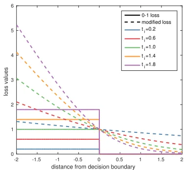
L(.)is a 0-1 misclassification function. Since the objective function of (10) is piecewise constant and discontinuous, the problem is NP-hard and in practice is approximated using surrogate loss (Maibing and Igel 2015). Here, we approxi-mate the solution to problem (10) using a modified logistic regression.
The easiest way to approximate (10) is to replace the 0-1 lossL(.)with a logistic loss. For simplicity of notation, we replace argmin
l
zilwithl∗={−1,1}. Therefore, we have:
min
Wj,bj
X
(xi,yi)∈Sj
tilog(1 +e−(l
∗(WTx
i−b))). (11)
Objective function in problem (11) is a convex function and one can easily optimize it using any gradient-based algo-rithm.However, implementation-wise, one might be inter-ested in using highly optimized existing toolboxes for lo-gistic regression such as liblinear (Fan et al. 2008). As per our search, no toolbox has the option for instance based cost-sensitive binary classification such as in (11). There-fore, we propose the following useful heuristic to use. For
-2 -1.5 -1 -0.5 0 0.5 1 1.5 2
distance from decision boundary 0
1 2 3 4 5 6
loss values
0-1 loss modified loss t
i=0.2
ti=0.6 ti=1.0 t
i=1.4
ti=1.8
Figure 2: 0-1 loss and our proposed surrogate loss functions for different sample weights. Intuitively, as cost of a sam-ple gets higher, the slope of surrogate loss gets steeper and essentially making it easier to classify.
each datapoint multiply it’s features and augmented bias by the misclassification cost of the datapoint (instead ofxi we
feedti×[xi, 1]) and then feed it to the toolbox. The
in-tuition is that the shape of loss function changes such that the loss for misclassified samples with higher costs (heavy samples) rises faster as they get further away from decision boundary(f(x) = 0) than the samples with lower costs (light samples). This still makes the loss function a surrogate to original 0-1 loss. Figure 2 shows 0-1 loss functions and our proposed modification.
OHMR for Multi-response Regression Univariate
Binary Trees
In univariate regression trees, the decision function at a split node is fj = sign(xPj −bj). This formulation is
simi-lar to problem (10) in which all the possible combinations of feature and threshold are O(Njp). In this case, the
so-lution can be found efficiently in O(Njp)by using an
in-cremental algorithm. We are interested in solving (10) with fj = sign(xP −b). This is a selection of a feature and
threshold. Again similar to section case of splitting a uni-variate node, there areO(N)available thresholds along each feature andO(N p)in total. One needs to calculate error for each threshold along a feature and the error. Error of left child is equal to summationEi =P
i
i0=1zi−10 (it is because
zl
i is equal to error of sample sent tolthchild andl = −1
corresponds to left child). Therefore, by shifting indexes, we have Ei = Ei +zi−1 which in practice is calculating
sincezilis one dimensional, computational complexity does not depend on the dimensionality ofyi.
OHMR for Classification Multivariate Binary
Trees
In order to tackle a classification problem, 0-1 loss misclas-sification can be used instead of regression loss in (6) and follow the procedure to problem (9). It is trivial to see that zl
i at the node is either 0 or 1 (because the loss function
produces 0 or 1). Therefore, it is possible to have similar costs for several children while in the regression case zl i
can be any positive real value. Further for case of classifi-cation binary trees, by following the same analysis as for case of binary regression trees, it can be seen that sample costtibecomes either0or1. Essentially meaning the
prob-lem only depends on samples that have sample cost of1; hence, leading to a binary classification(TAO algorithm in (Carreira-Perpi˜n´an and Tavallali 2018)).
An alternative method to solve a classification problem using regression loss is to change the categorical variable outputs to hot-one-vectors. By doing so sample costs at the nodes will remain positive real value; hence, termi-nating confusion caused by0 cost samples. For classifica-tion experiments, in this paper the second method is ap-plied. However, focus of the current paper is on regres-sion problems and We are not trying to address classifi-cation in this paper, as it has been done in some previous work (Norouzi et al. 2015b; 2015a; Frosst and Hinton 2017; Carreira-Perpi˜n´an and Tavallali 2018; Bertsimas and Dunn 2017). However, we are trying to show the capabilities of OHMR in treating classification as regression.
Computational Complexity
Theorem 2 (computational complexity). Computational
complexity of one pass of OHMR over the k-ary tree (k
de-notes the number of children each node has) structure is O(Dg(N, p) +kD2N h(p)), if following condition holds for g(N, p):
X
j
g(Nj, p)≤g(N, p)s.t
(P
jNj≤N
Nj, N∈Z+ . (12)
Here g(.) and h(.) are the computational complexities of
training over N samples and evaluating a sample for the
model at the nodes, respectively.
Proof. First, we define the computational complexity of one pass over the tree.
D
X
n=1 X
depth(j)=n
g(Nj, p) +k(D−n)Njh(p). (13)
Here, the index of first summation is over the depth of the tree and second summation is over the nodes at the same depth of n. depth(j) = n denotes index of any node j that is at depth n. First term, g(Nj, p) is due to training
model at node j. Second term, k(D −n)Njh(p) is due
to propagating each sample (these are Nj samples) down
each k children (which are a subtree of depth D − n)
and calculating its costs at node j. Since each input sam-ple in the structure can only follow a fixed path, at a cer-tain depth, a sample can be present in at most only at one node. As a result, we have P
depth(j)=nNj ≤ N.
Hence, P
depth(j)=ng(Nj, p) ≤ g(N, p). This leads to
the fact that at depth n, we have P
depth(j)=ng(Nj, p) +
k(D − n)Njh(p) ≤ g(N, p) + k(D − n)N h(p). So,
the total computational complexity of training models is PD
n=1g(N, p) + k(D − n)N h(p) = Dg(N, p) +
kD(D2+1)N h(p). Therefore, asymptotically total computa-tional complexity isO(Dg(N, p) +kD2N h(p)).
computational complexity of applying OHMR to regres-sion binary trees: for multivariate case: solving a logistic loss function using truncated Newton method costsO(αN p) (Hsia, Zhu, and Lin 2017) (g(N, p) = αN p). α is the number of iterations performed. Evaluating each split node takesh(p) =p. Therefore, by plugginghandgin theorem 2, OHMR’s learning complexity isO(DαN p+ 2D2N p)).
The algorithm is linear on the number of samples. Simi-larly, for univariate case, the computational complexity is O(DN p+ 2D2).
Experiments and Results
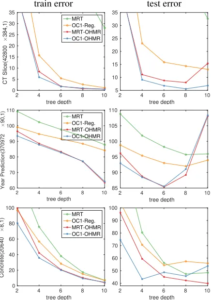
In this section, we present results of experiments to show the merits of our proposed method. In all these experiments, OHMR is applied to an induced MRT or OC1-Reg tree. MRT is similar to the CART algorithm, except that the this algorithm is applied to a multi-response tree like the work in (De’Ath 2002). OC1-reg is also OC1 optimization algorithm for a single oblique tree applied for multi-response regres-sion. To the best of our knowledge, it is the first time this method has been applied to create one OC1 tree for a multi-response regression task. In all experiments, at the split op-timization, logistic regression was trained using (Fan et al. 2008) library. In each figure, the dataset and its dimension-ality is written left to the figure asdatasetname(N×p, d). All reported errors are mean squared error.
The optimized MRT and OC1-Reg are called MRT-OHMR and OC1-MRT-OHMR, respectively. Maximum number of allowed iterations over tree was set to10. As a reminder, we mention that the OHMR model for the experiments is the model introduced for multivariate trees.
Comparison With Regression Trees
During the regression experiments, the datasets were ran-domly partitioned to 64% train, 16% validation and 20% test sets. Concrete Compressive Strength(CCS), Airfoil, CT slice localization and California housing(CADATA) datasets were downloaded from (Dheeru and Karra Taniskidou 2017). Classification datasets and regression dataset of Year Prediction were downloaded from (Chang and Lin 2011).
train error test error
2 4 6 8 10
tree depth 0
5 10 15 20 25 30 35
CT Slice(42800
×
384,1)
MRT OC1-Reg. MRT-OHMR OC1-OHMR
2 4 6 8 10
tree depth 5
10 15 20 25 30 35
2 4 6 8 10
tree depth 60
70 80 90 100 110
Year Prediction(370972
×
90,1) MRTOC1-Reg. MRT-OHMR OC1-OHMR
2 4 6 8 10
tree depth 85
90 95 100 105 110
2 4 6 8 10
tree depth 0
20 40 60 80 100
Concrete(20640
×
8,1)
MRT OC1-Reg. MRT-OHMR OC1-OHMR
2 4 6 8 10
tree depth 40
50 60 70 80 90 100
Figure 3: Train and test errors(mean squared error) of the proposed method as compared to other greedy algorithms in the literature. OHMR has achieved the smallest test error in all 3 datasets, winning all time in 2 datasets and best train in all of them.
and picking the best tree among trees of different depths. In addition, the algorithm is also fast and usually takes 25 seconds to optimize a tree of depth 8 over a dataset like CT Slice using a device with 4 core i7 cpu and 8 GB of ram.
Comparison With Forest Models
The fact with the regression trees is that they are fast in query complexity. Hence, one important problem is to see if an oblique tree can do as good as, or on par as, a forest model while preserving the tree’s faster query complexity. To check this, we compared OHMR with a few recently pro-posed forest models. For a fair comparison, we followed the same dataset partition as in (Begon, Joly, and Geurts 2017; Li and Martin 2017) for each dataset. The query complexity consists of the number of element-wise multiplications and additions needed to propagate a sample down the trees or forest. The number of parameters consists of all existing pa-rameters throughout the model nodes. Methods that do not fit inside the plots are put on the boundaries of them.
For CADATA, dataset was partitioned into66%train and 34%test sets, each experiment was done 10times and the averages of the test errors are reported. For Airfoil and Con-crete, datasets were partitioned into60%train and40%test
sets and each experiment was conducted20times. OHMR was applied to trees of depth2to10. The errors of these trees are reported as a function of query complexity and number of parameters; see figure 4.
In Figure 4, red and blue lines show MRT-OHMR and OC1-OHMR,respectively. Each two consecutive dots on the line represent two trees at consecutive depths. The trees on the lines start from depth 2 and increases up to depth 10. Huber, and Tukey were forest models from (Li and Mar-tin 2017). The forests in this paper were first induced by a random forest of1000trees as a kernel for non-parametric models. Then the non-parametric models were used to pre-dict target values with respect to different loss functions such as Huber (Huber and others 1964) and Tukey (Huber 2011). Random forest (RF) in all datasets consist of 100 trees of depth 9. ET100, ET10, ET1, GIF10, GIF1 are forest mod-els from (Begon, Joly, and Geurts 2017). ET100 is a ran-dom forest of1000fully grown trees. ET10 and ET1 are the same as ET100, except that they are built such that they have as10%and1%many nodes as ET100, respectively. GIF10 and GIF1 are the authors proposed method greedily induc-ing forests that has as10%and1%many nodes as ET100, respectively. Since the information about query complexity of ET100, E10 and ET1 were not available, they were not reported in figures consisting of query complexity.
The query complexity and size of other Huber and Tukey forests are estimated in the experiments based on the mini-mum needed query complexity or number of parameters re-ported in the (Huber and others 1964). Figure 4 ,the graphs in the left column, demonstrates the fact that a single oblique tree can outperform, or do almost as good as, a forest model. However, in all cases, the query complexity of OHMR is or-ders of magnitude smaller.
Figure 4,the graphs in the right column, shows the per-formance of different models with respect to the number of parameters of each model. As a tree grows larger, the num-ber of its parameters increase exponentially. However, still with small trees, OHMR was able to achieve comparable or smaller error compared to the forest models.
Compressed multivariate trees One direct application of OHMR is to use it toward building sparse multivariate trees by imposingl1penalty over the weightsλj||Wj||1of each
node.λjis the regularization parameter for each node. This
helps achieve trees with smaller size and faster query com-plexity, specifically useful for large datasets such as CT slice. To do so, two general approaches can be followed. One is to set λj equal for all nodes and similar to lasso
(Hastie, Tibshirani, and Friedman 2009) follow the regular-ization path (increaseλjfrom a small value to a large value)
and at each value ofλjoptimizing the tree. However, since
the lower level nodes in the tree receive smaller number of samples, their weights get sparser with smaller values ofλj,
resulting in subtrees with no samples; hence, a post process-ing procedure is needed to prune the inactive subtrees (e.g. (Carreira-Perpi˜n´an and Tavallali 2018)). Second approach is to setλjfor each node individually. To do so, a balance
102 103 10 2 3 4 5 CADATA(20640 × 8,1) test error ×10-1 MRT-OHMR OC1-OHMR GIF 10% GIF 1% RF
102 103 104 105 2
3 4 5×10
-1 MRT-OHMR OC1-OHMR ET 100% ET 10% ET 1% GIF 10% GIF 1% RF
102 103
5 10 15 20 Airfoil(1503 × 5,1) test error MRT-OHMR OC1-OHMR RF QRF huber tuckey
102 103
5 10 15 20 MRT-OHMR OC1-OHMR RF QRF huber tuckey
102 103
40 50 60 70 80 90 Concrete(1030 × 8,1) test error MRT-OHMR OC1-OHMR RF QRF huber tuckey
102 103
40 50 60 70 80 90 MRT-OHMR OC1-OHMR RF QRF huber tuckey
query complexity # parameters
Figure 4: Test error(mean squared error) versus query com-plexity and number of parameters are shown over different data sets for OHMR and several forest models.
level nodes do not get heavily penalized. For this we set λj/Nj =Cin whichCis a constant value. As a result,λj
will change proportional to number of samples the node re-ceives. Then, follow the regularization path based onC, in-creasingCfrom a small value to a large one and optimize the tree for each value ofC. In practice, we noticed the second approach results in faster and similar size trees compared to first approach. Further, each node gets similar sparsity ra-tio to other nodes through the tree; hence resulting in no structural changes. Nodes may occasionally get empty (un-less regularization penalty is high). Note that the rejection step must not be applied, otherwise, updates are rejected and sparsity is not achieved. From the trees along the regulariza-tion path, the best tree can be picked by cross-validaregulariza-tion or in case the validation set is not provided, by looking at the train error of the trees versus their sparsity and picking the sparsest tree among trees with lowest train error. The second approach experiment is applied over CT slice and is com-pared with other forest, nearest neighbor and radial basis function (RBF) models. Same data partition as (Begon, Joly, and Geurts 2017) was followed. Figure 5 shows different methods compared to OHMR. Both top graphs of figure 5 show that sparse OHMR was able to achieve mostly smaller test error while having order of exponent faster query and
101 102 103 104 105 average operations per sample 10 17 31 56 100 test error 1 2 3 4 5 6 7 10 12 depth: 2 depth: 4 depth: 6 depth: 8 depth:10 MRT-OHMR:1 OC1-OHMR:1 MRT-OHMR:2 OC1-OHMR:2 MRT OC1-reg other
101 102 103 104 105 106 number of parameters 10 17 31 56 100 test error 1 2 3 4 5 6 7 8 9 10 11 12
103 104 105 106
λ 100 101 102 103 # nodes depth: 2 depth: 4 depth: 6 depth: 8 depth: 10 initial tree:OC1 initial tree:MRT MRT-OHMR OC1OHMR
10-5 10-4 10-3 10-2 λ
j / Nj
100 101 102 103 # nodes depth: 2 depth: 4 depth: 6 depth: 8 depth: 10 initial tree:OC1 initial tree:MRT MRT-OHMR OC1-OHMR
Figure 5: Test error versus query complexity and size are shown over CT slice dataset in top two curves. Other models are shown by × symbol and a number beside it. MRT-OHMR:1, OHMR:1 and MRT-OHMR:2, OC1-OHMR:2 correspond to first and second setup of exper-iments mentioned in compressed trees paragraph respec-tively. 1 is nearest neighbor. 2 is a bagging ensemble of 250 trees of depth 10. Sampling rate was0.7. models 3,4,5,6 and 7 are RBF models with 100,200,300,400,500 basis func-tions and used as transformation to a linear regression. Gaus-sian functions with same variance were used and centers were found using k-means. 8,9,10,11,12, are ET100, ET10, GIF10, ET1 and GIF1 respectively. The bottom two curves show number of nodes remained asλj/Nj or λincreases.
Left and right figures of second row correspond to first and second setup of experiments mentioned in compressed trees paragraph respectively. The black horizontal line displays the selected tree models shown in the bottom two curves.
smaller size. Some nodes getting empty due to receiving no training samples were pruned after the experiment proce-dure. The bottom two graphs of figure 5 have explored num-ber of nodes through the experiments procedure. # nodes is the number of nodes.
OHMR Applied to Axis-aligned Regression Trees
Table 1: Test classification accuracy (avg±stdev) for dif-ferent methods and datasets (sample size×dimensionality, # classes). All models are axis-aligned trees.
DATA SET DEPTH MRT OHMR OCT
BREAST 2 90.8±1.2 92.9±2.0 91.9
CANCER 3 92.9±0.5 93.2±1.2 91.5
(569×30,2) 4 92.8±0.6 93.1±0.5 91.5
SPAMBASE 2 82.5±2.4 85.9±0.9 84.3
(4601×57,2) 3 87.2±1.1 89.1±1.0 86.0
4 89.7±0.9 90.4±0.7 86.1
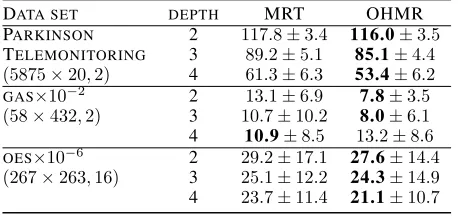
Table 2: Mean squared error over test set (avg±stdev) for different methods and datasets (sample size× dimension-ality, # output dimensionality). All models are axis-aligned trees.
DATA SET DEPTH MRT OHMR
PARKINSON 2 117.8±3.4 116.0±3.5
TELEMONITORING 3 89.2±5.1 85.1±4.4
(5875×20,2) 4 61.3±6.3 53.4±6.2
GAS×10−2 2 13.1±6.9 7.8±3.5
(58×432,2) 3 10.7±10.2 8.0±6.1
4 10.9±8.5 13.2±8.6
OES×10−6 2 29.2±17.1 27.6±14.4
(267×263,16) 3 25.1±12.2 24.3±14.9
4 23.7±11.4 21.1±10.7
Classification as Regression
In this section, we present examples on how a classification problem can be handled as a regression using OHMR. The target classes are changed to hot-one-vector in which the di-mension is 1 if the class of a point belongs to that dimen-sion and other dimendimen-sions are zero. This enables a regres-sion tree to handle a classification problem in the context of regression. Datasets are from in (Chang and Lin 2011). Our proposed method was able to improve significantly over test and train accuracies and outperform recently introduced op-timization method in (Norouzi et al. 2015a) and greedy tree in (Norouzi et al. 2015b) called non-greedy and CO2, re-spectively. Specifically, in MNIST, OHMR was able to pass accuracy90%test accuracy at depth of 4 and also achieve the best accuracy of95.39%at depth 12.
Conclusion
This paper tackled the problem of optimizing a multi-response regression tree through a meta-algorithm that pro-poses general procedure for optimizing any hierarchical (e.g., k-ary trees) structure for regression (OHMR). OHMR provides opportunity for also learning sparse weights at the nodes. Inspired by (Jordan and Jacobs 1994), OHMR is done by iterating over the nodes and optimizing one at a time which leads to instance-based cost-sensitive classification at the split nodes and a regular regression problem at the leaf nodes. Proposed method has an efficient training procedure making it possible to scale the algorithm to larger datasets
5 10 15
tree depth 65
70 75 80 85
test accuracy
connect4(67557 ×126,3)
5 10 15
tree depth 60
70 80 90 100
test accuracy
MNIST(60000×784,10)
MRT OC1-Reg. CO2 non-greedy MRT-OHMR OC1-OHMR
5 10 15
tree depth 60
70 80 90 100
test accuracy
Covtype(581012 ×53,7)
5 10 15
tree depth 60
70 80 90 100
test accuracy
Pendigits(7494 ×16,10)
Figure 6: Test accuracy of the proposed method compared to other greedy and optimization algorithms in the literature. OHMR has almost achieved the best test accuracy in most data sets.
and models. OHMR is also capable of competing with exist-ing ensemble methods and even achievexist-ing smaller test error, hence, possibility of essentially decreasing query complex-ity and size of the model. Because of OHMR other research topics using trees such as using other loss functions toward other tasks such as density estimation, manifold learning, multi-class labeling and using more complicated models at the split nodes have now become easily possible. All that is needed is to approximate or solve problem (9) for any given task.
Acknowledgment
Peyman Tavallali’s research contribution to this paper was carried out at the Jet Propulsion Laboratory, California Insti-tute of Technology, under a contract with the National Aero-nautics and Space Administration.
References
Begon, J.-M.; Joly, A.; and Geurts, P. 2017. Globally in-duced forest: A prepruning compression scheme. In
Inter-national Conference on Machine Learning, 420–428.
Bennett, K. P. 1992. Decision tree construction via linear programming. InProc. 4th Midwest Artificial Intelligence and Cognitive Sience Society Conference, 97–101.
Bennett, K. P. 1994. Global tree optimization: A non-greedy decision tree algorithm. Computing Science and Statistics 26:156–160.
Bertsimas, D., and Dunn, J. 2017. Optimal classification trees. Machine Learning106(7):1039–1082.
Breiman, L. J.; Friedman, J. H.; Olshen, R. A.; and Stone, C. J. 1984. Classification and Regression Trees. Belmont, Calif.: Wadsworth.
Breiman, L. 1996. Bagging predictors. Machine learning 24(2):123–140.
Breiman, L. 2001. Random forests. Machine learning 45(1):5–32.
Carreira-Perpi˜n´an, M. ´A., and Tavallali, P. 2018. Alternat-ing optimization of decision trees, with application to learn-ing sparse oblique trees. InAdvances in Neural Information
Processing Systems, 1219–1229.
Chang, C.-C., and Lin, C.-J. 2011. Libsvm: a library for support vector machines. ACM transactions on intelligent systems and technology (TIST)2(3):27.
Criminisi, A., and Shotton, J. 2013. Decision Forests for
Computer Vision and Medical Image Analysis. Advances in
Computer Vision and Pattern Recognition. Springer-Verlag. De’Ath, G. 2002. Multivariate regression trees: a new technique for modeling species–environment relationships.
Ecology83(4):1105–1117.
Dheeru, D., and Karra Taniskidou, E. 2017. UCI machine learning repository.
Fan, R.-E.; Chang, K.-W.; Hsieh, C.-J.; Wang, X.-R.; and Lin, C.-J. 2008. Liblinear: A library for large linear classifi-cation.Journal of machine learning research9(Aug):1871– 1874.
Freund, Y.; Schapire, R.; and Abe, N. 1999. A short intro-duction to boosting.Journal-Japanese Society For Artificial Intelligence14(771-780):1612.
Frosst, N., and Hinton, G. 2017. Distilling a neural network into a soft decision tree. arXiv preprint arXiv:1711.09784. Garofalakis, M.; Hyun, D.; Rastogi, R.; and Shim, K. 2003. Building decision trees with constraints. Data Mining and
Knowledge Discovery7(2):187–214.
Hastie, T.; Tibshirani, R.; and Friedman, J. H. 2009. The elements of statistical learning: data mining, inference, and prediction. New York, NY: Springer, second edition. Heath, D.; Kasif, S.; and Salzberg, S. 1993. Induction of oblique decision trees. InIJCAI, volume 1993, 1002–1007. Hsia, C.-Y.; Zhu, Y.; and Lin, C.-J. 2017. A study on trust region update rules in newton methods for large-scale linear classification. InAsian Conference on Machine Learning, 33–48.
Huber, P. J., et al. 1964. Robust estimation of a location parameter. The annals of mathematical statistics35(1):73– 101.
Huber, P. J. 2011. Robust statistics. InInternational Ency-clopedia of Statistical Science. Springer. 1248–1251. Ikonomovska, E.; Gama, J.; and Dˇzeroski, S. 2011. Incre-mental multi-target model trees for data streams. In Pro-ceedings of the 2011 ACM symposium on applied comput-ing, 988–993. ACM.
Jordan, M. I., and Jacobs, R. A. 1994. Hierarchical mix-tures of experts and the em algorithm. Neural computation 6(2):181–214.
Kocev, D.; Dˇzeroski, S.; White, M. D.; Newell, G. R.; and Griffioen, P. 2009. Using single-and multi-target regression trees and ensembles to model a compound index of vegeta-tion condivegeta-tion. Ecological Modelling220(8):1159–1168. Kocev, D.; Vens, C.; Struyf, J.; and Dˇzeroski, S. 2013. Tree ensembles for predicting structured outputs.Pattern
Recog-nition46(3):817–833.
Laurent, H., and Rivest, R. L. 1976. Constructing optimal binary decision trees is np-complete.Information processing letters5(1):15–17.
Levati´c, J.; Ceci, M.; Kocev, D.; and Dˇzeroski, S. 2014. Semi-supervised learning for multi-target regression. In In-ternational Workshop on New Frontiers in Mining Complex Patterns, 3–18. Springer.
Li, A. H., and Martin, A. 2017. Forest-type regression with general losses and robust forest. InInternational Conference
on Machine Learning, 2091–2100.
Loh, W.-Y., and Shih, Y.-S. 1997. Split selection methods for classification trees. Statistica sinica815–840.
Maibing, S. F., and Igel, C. 2015. Computational complex-ity of linear large margin classification with ramp loss. In Artificial Intelligence and Statistics, 259–267.
Murthy, S. K.; Kasif, S.; and Salzberg, S. 1994. A system for induction of oblique decision trees. Journal of artificial intelligence research2:1–32.
Nijssen, S., and Fromont, E. 2007. Mining optimal decision trees from itemset lattices. InProceedings of the 13th ACM SIGKDD international conference on Knowledge discovery
and data mining, 530–539. ACM.
Norouzi, M.; Collins, M.; Johnson, M. A.; Fleet, D. J.; and Kohli, P. 2015a. Efficient non-greedy optimization of de-cision trees. InAdvances in Neural Information Processing
Systems, 1729–1737.
Norouzi, M.; Collins, M. D.; Fleet, D. J.; and Kohli, P. 2015b. Co2 forest: Improved random forest by con-tinuous optimization of oblique splits. arXiv preprint
arXiv:1506.06155.
Quinlan, J. R. 2014. C4. 5: programs for machine learning. Elsevier.
Struyf, J., and Dˇzeroski, S. 2005. Constraint based induction of multi-objective regression trees. InInternational
Work-shop on Knowledge Discovery in Inductive Databases, 222–
233. Springer.