Efficient and Scalable Multi-Task Regression on Massive Number of Tasks

The Thirty-Third AAAI Conference on Artificial Intelligence (AAAI-19)

Efficient and Scalable Multi-Task Regression on Massive Number of Tasks

Xiao He

[email protected]

Francesco Alesiani

Ammar Shaker

Abstract

Many real-world large-scale regression problems can be for-mulated as Multi-task Learning (MTL) problems with a mas-sive number of tasks, as in retail and transportation domains. However, existing MTL methods still fail to offer both the generalization performance and the scalability for such prob-lems. Scaling up MTL methods to problems with a tremen-dous number of tasks is a big challenge. Here, we propose a novel algorithm, named Convex Clustering Multi-Task regression Learning (CCMTL), which integrates with con-vex clusteringon thek-nearest neighbor graph of the predic-tion models. Further, CCMTL efficiently solves the under-lying convex problem with a newly proposed optimization method. CCMTL isaccurate,efficientto train, and empir-icallyscales linearlyin the number of tasks. On both syn-thetic and real-world datasets, the proposed CCMTL outper-forms seven state-of-the-art (SoA) multi-task learning meth-ods in terms of prediction accuracy as well as computational efficiency. On a real-world retail dataset with23,812tasks, CCMTL requires only around30seconds to train on a single thread, while the SoA methods need up to hours or even days.

Introduction

Multi-task learning (MTL) is a branch of machine learn-ing that aims at exploitlearn-ing the correlation among tasks. To achieve this, the learning of different tasks is per-formed jointly. It has been shown that learning task re-lationships can transfer knowledge from information-rich tasks to information-poor tasks (Zhang and Yeung 2014) so that overall generalization error can be reduced. With this characteristic, MTL has been successfully applied in use cases ranging from Transportation (Deng et al. 2017) to Biomedicine (Li, He, and Borgwardt 2018).

Various multi-task learning algorithms have been pro-posed in the literature, Zhang and Yang (Zhang and Yang 2017) wrote a comprehensive survey on state-of-the-art (SoA) methods. For instance, feature learning approach (Ar-gyriou, Evgeniou, and Pontil 2007) and low-rank approach (Ji and Ye 2009; Chen, Zhou, and Ye 2011) assume all the tasks are related, which may not be true in real-world ap-plications. Task clustering approaches (Bakker and Heskes 2003; Jacob, Vert, and Bach 2009; Kumar and Daume III Copyright c2019, Association for the Advancement of Artificial Intelligence (www.aaai.org). All rights reserved.

2012) can deal with the situation where different tasks form clusters. However, despite being accurate, these latter meth-ods are computationally expensive for problems with a large number of tasks.

In real-world regression applications, the number of tasks can be tremendous. For instance, in the retail market, shops’ owners would like to forecast the sales amount of all the products based on the historical sales information and exter-nal factors. For a typical shop, there are thousands of prod-ucts, where each product can be modeled as a separate re-gression task. In addition, if we consider large retail chains, where the number of shops in a given region is in the order of hundreds, the total number of learning tasks easily grows up to hundreds of thousands. A similar scenario can also be found in other applications, e.g. demand prediction in trans-portation, where each task is one public transport station de-mand in a city at a certain time per line. Here, at least tens of thousands of tasks are expected.

In all these scenarios, MTL approaches that exploit rela-tionships among tasks are appropriate. Unfortunately most of existing SoA multi-task learning methods cannot be ap-plied, because either they are not able to cope with task heterogeneity or are too computationally expensive, scaling super-linearly in the number of tasks.

To tackle these issues, this paper introduces a novel al-gorithm, named Convex ClusteringMulti-Task regression Learning (CCMTL). It integrates the objective of convex clustering (Hocking et al. 2011) into the multi-task learn-ing framework. CCMTL is efficient with linear runtime in the number of tasks, yet provides accurate prediction. The detailed contributions of this paper are fourfold:

1. Model:A new model for multi-task regression that in-tegrates withconvex clusteringon thek-nearest neigh-bor graph of the prediction models;

2. Optimization Method: A new optimization method for the proposed problem that is proved to converge to the global optimum;

3. Accurate Prediction: Accurate predictions on both synthetic and real-world datasets in retail and trans-portation domains which outperform eight SoA multi-task learning methods;

On a real-world retail dataset with23,812 tasks, the algorithm requires only around 30 seconds to termi-nate, whereas SoA methods typically need up to hours or even days.

Over the remainder of this paper, we introduce the proposed algorithm, present the mathematical proofs and a comprehensive experimental setup that benchmarks CCMTL against the SoA on multiple datasets. Lastly, we discuss related works and conclude the paper.

The Proposed Method

Let us consider a dataset withTregression tasks{Xt, Yt}=

{(xti, yti) : i ∈ {1, ..., Nt}}for each taskt ∈ {1, ..., T}.

Xt ∈RP×Nt _{consists ofN}

tsamples andPfeatures, while

Yt ∈ R1×Nt is the target for task t. There are totallyN

samples, whereN =PT_t=1Nt. We consider linear models

in this paper. Let W = (WT

1, ..., WTT) ∈ RT×P, where

Wt∈RP×1represent the weight vector for taskt.

Model

Task clustering MTL methods learns the task relationships by integrating withk-means (Jacob, Vert, and Bach 2009; Zhou, Chen, and Ye 2011b) or matrix decomposition (Ku-mar and Daume III 2012). Unfortunately, these methods are expensive to train, making them impractical for problems with a massive number of tasks.

Recently,convex clustering(Hocking et al. 2011) has at-tracted much attention. It solves clustering of data X as a regularized reconstruction problem:

min

U

1

2||X−U||

2 F+

λ

2

X

i,j∈G

||Ui−Uj||2 (1)

whereUiis the new representation for theith sample, andG

is the k-nearest neighbor graph onX. It is critical to note that the edge terms involve the `2 norm, not the squared

`2 norm, which is essential to achieve clustering. Further, it has been shown thatconvex clusteringis efficient with lin-ear scalability (Chi and Lange 2015; Shah and Koltun 2017; He and Moreira-Matias 2018).

Suppose we have a noisy observation of the true predic-tion modelsZ ∈ RT×P; we would like to learn less noisy

modelsW byconvex clustering:Z andW would take the role ofXandU in Problem (1), respectively. SinceZis not available in practice and the target of MTL is the prediction, we use the prediction error instead of the reconstruction er-ror and form the problem as follows:

min

W

1 2

T X

t=1

||W_tTXt−yt||22+

λ

2

X

i,j∈G

||Wi−Wj||2 (2)

whereλis a regularization parameter andGis thek-nearest neighbor graph on the prediction models learned indepen-dently for each task.

Note that if we use`1 norm||Wi −Wj||1 as the regu-larizer, Problem (2) equals to the Fused Multi-task Learning (FuseMTL) (Zhou et al. 2012; Chen et al. 2010). However, it has been shown that`2norm works better for clustering in most cases (Hocking et al. 2011). This improvement is also confirmed for MTL in the experimental section.

Optimization

The Problem (2) lies in the general framework of Net-workLasso (Hallac, Leskovec, and Boyd 2015), and hence it could be solved by NetworkLasso, which is based on the general alternating direction method of multipliers (ADMM). However, NetworkLasso is not specifically de-signed for the multi-task regression problem. Further, in our experiments, we find its performance on single thread is rather slow and the convergence is affected by its hyperpa-rameters.

Chi and Lange (Chi and Lange 2015) propose an alternat-ing minimization algorithm (AMA) for convex clustering, which has been shown to be faster than the ADMM based method. Even if the approach can also be applied to solve Problem (2), its convergence is only guaranteed under cer-tain conditions. Later, Wang et al. (Wang et al. 2016) pro-pose a variation of the AMA method forconvex clustering. We test this method to solve Problem (2), but the conver-gence is not always empirically achieved.

Shah and Koltun (Shah and Koltun 2017) propose an ef-ficient method forcontinuous clusteringwith a non-convex regularization function. Inspired by this method, we propose a new efficient algorithm for Problem (2) by iteratively solv-ing a structured linear system.

First we introduce an auxiliary variable L = {li,j} for

each connection between nodeiandjin graphG,li,j≥0,

and we form the following new problem:

min

W,L

1 2

T

X

t=1

||WtTXt−yt||22+

λ

2 X

i,j∈G

(li,j||Wi−Wj||2 2+

1 4l

−1

i,j) (3)

Theorem 1. The optimal solutionW∗ of Problem (2) and Problem (3) are the same if

li,j =

1 2||Wi−Wj||2

(4)

Proof. Theorem 1 can be simply proved by substituting Eq. (4) into Problem (3), obtaining Problem (2).

Intuitively, Problem (3) learns the weights li,j for the

squared`2norm regularizer||Wi−Wj||22as in Graph regu-larized Multi-task Learning (SRMTL) (Zhou, Chen, and Ye 2011b). With noisy edges, squared`2norm forces uncorre-lated tasks to be close, while`2norm is more robust which is confirmed for MTL in the experimental section.

To solve Problem (3), we optimizeW andLalternately. WhenW is fixed, we get the derivative of Problem (3) with respect tolij, set it to zero and get the update rule as shown

in Eq. (4).

WhenLis fixed, Problem (3) equals to

min

W

1 2

T X

t=1

||W_tTXt−yt||22+

λ

2

X

i,j∈G

(li,j||Wi−Wj||22) (5)

In order to solve Problem (5), let us defineX ∈_RT P×N

as a block diagonal matrix

X=



 

X1 . ._.

XT 

defineY ∈R1×N as a row vector

Y = [y1, . . . , yT],

and defineV ∈RT P×1as a column vector

V =



 

W1 .. .

WT 

 

Then, Problem (5) can be rewritten as:

min

V

1 2||V

T_X−y||2 2+

λ

2

X

i,j∈G

(li,j||V((ei−ej)⊗IP)||22)

(6) whereei ∈ RT is an indicator vector with theith element

set to1and others0andIPis an identity matrix of sizeP.

Setting the derivative of Problem (6) with respect toV to zero, the optimal solution ofV can be obtained by solving the following linear system:

(A+B)V =C (7) whereA= (λP

i,j∈Gli,j(ei−ej)(ei−ej)T)⊗IP,B =

XXT,C=XYT, andW is derived by reshapingV.

Convergence Analysis

Theorem 2. Alternately updating Eq. (4) and Eq. (7) onL

andW converges to a global optimum of Problem (2).

Proof. Problem (3) is biconvex onW andL. Therefore, al-ternately updating Eq. (4) and Eq. (7) will converge to a local minimum (Beck 2015). Here we prove it in a different way. We show that this method is a contracting mapM, so that

d(M(x), M(y)) ≤ d(x, y). LetJ(W, L)equals to the ob-jective function defined in Problem (3). We used(x, y) =

|J(W, L)−J(W0, L0)|, withx = (W, L), y = (W0, L0). We then demonstrate that

|J(W+, L+)−J(W∗, L∗)| ≤ |J(W−, L−)−J(W∗, L∗)|

where1 _(W∗_{, L}∗_{) = M(W}∗_{, L}∗_{) because (W}∗_{, L}∗_{) is a}

stationary point. We define (W+_{, L}+_{) = M(W}−_{, L}−_),

where(W−, L−),(W+, L+)are the variables before and after the mapping. Our mappingMis composed of two steps

W− _→W+_{followed byL}−_→L+_{. We show that the first} step is a contraction and that the same is true also for the sec-ond step, and therefore for their composition. The first step updates theW− using the gradient of ∇WJ(W, L−) = 0

and finds the optimal minimum having fixedL−, thus

|J(W+, L−)−J(W∗, L∗)| ≤ |J(W−, L−)−J(W∗, L∗)|

The second step updateslij such that ∇LJ(W+, L) = 0,

thus

|J(W+, L+)−J(W∗, L∗)| ≤ |J(W+, L−)−J(W∗, L∗)|,

where the reduction is both obtained by a gradient descent step or by direct solution sinceJ is convex in the two vari-ables separately. By applying composition of the two opera-tions we have

|J(W+, L+)−J(W∗, L∗)| ≤ |J(W+_{, L}−_)−J(W∗_{, L}∗_)|

≤ |J(W−_{, L}−_)−J(W∗_{, L}∗_)|

1

the superscript *,+ and - indicate the optimal, the starting and the next update values of the variablesWandL.

Algorithm 1:CCMTL

Input :{Xt, Yt}fort={1,2, ..., T},λ

Output:W ={W1, ..., WT}

1 fort←1toTdo

2 SolveWtby Linear Regression on{Xt, Yt}

3 end

4 Constructk-nearest neighbor graphGonW; 5 whilenot convergedo

6 UpdateLusing Eq. (4);

7 UpdateW by solving Eq. (7) using CMG (Ioannis, Miller, and Tolliver 2011);

8 end 9 returnW;

which proves the convergence of the method.

Suppose the method converges to a local optimal solution (W∗, L∗)of Problem (3). SinceL∗satisfies Eq. (4),W∗is also optimal for Problem (2) according to Theorem 1. Prob-lem (2) is convex, thusW∗ is a global optimal solution of Problem (2).

Efficient and Scalable Implementation

CCMTL is summarized in Algorithm 1. Firstly, it initial-izes the weight vectorWtby performing Linear Regression

on each task tseparately. Then, it constructs thek-nearest neighbor graph GonW based on the Euclidean distance. Finally, the optimization problem is solved by iteratively up-datingLandWuntil convergence.

Solving the linear system in Eq. (7) involves inverting a matrix of sizeP T×P T, wherePis the number of features andT is the number of tasks. Direct inversion will lead to cubic computational complexity, which will not scale to a large number of tasks. However, there are certain properties of A andB in Eq. (7) that can be used to derive efficient implementation.

Theorem 3. A and B in Eq. (7) are both Symmetric and Positive Semi-definite andAis a Laplacian matrix.

Proof. Clearly,A andB are Symmetric. For each pair of edge(i, j)inG,(ei−ej)(ei−ej)Tis a Laplacian matrix by

definition. Since the summation of Laplacian matrices and multiplying a positive value to a Laplacian matrix are still Laplacian,λP

i,j∈Gli,j(ei−ej)(ei−ej)

T _{is a Laplacian}

matrix since λ ≥ 0 andlij ≥ 0. The Kronecker product

of a Laplacian matrix and an identity matrix will lead to a block diagonal matrix, where the diagonals are all Laplacian matrices. Therefore,Ais a Laplacian matrix and it is Posi-tive Semi-definite.Bis a dot product, therefore it is Positive Semi-definite as well.

Further, recent studies (Cohen et al. 2014; Kelner et al. 2013) show that linear systems with sparse Laplacian matri-ces can be solved in near-linear time. Among them, (Ioan-nis, Miller, and Tolliver 2011) proposed the Combinato-rial MultiGrid (CMG) algorithm, which is also a CG based method that utilizes the hierarchal structure of the Laplacian matrix. CMG empirically scales linearly w.r.t. the non-zero entries in the Laplacian matrix of the linear system.

Based on Theorem 3, A is a sparse Laplacian matrix. Therefore, we adopt CMG to solve Eq. (7) in CCMTL. Al-though,A+B is not a Laplacian matrix anymore, empir-ically we find out that CMG still converges fast and scales linearly in the number of tasks. We conjecture that this is due to the fact thatBis a structured block diagonal matrix.

The runtime of CCMTL consists of threefold: 1) Initial-ization ofW, 2)k-nearest neighbor graph construction, and 3) optimization of Problem (3). Clearly, initialization ofW

by linear regression is efficient and scales linearly on the number of tasks T. k-nearest neighbor graph construction naively scales quadratically toT. However, it is not the bur-den when using MATLAB’spdist2function even for a syn-thetic dataset with160,000tasks. CCMTL empirically con-verges fast within around30iterations. The majority of run-time is for solving the linear system in Eq. (7). The adopted CMG method scales empirically linearly in the number of non-zero entries inAandBin Eq. (7), which is linear toT.

Experiments

Comparison Methods

We compare our methodCCMTLwith several SoA meth-ods. As baselines, we compare with Single-task learning (STL), which learns a single model by pooling together the data from all the tasks and Independent task learning (ITL), which learns each task independently. These baselines rep-resent the two extreme hypothesis, full independence of the tasks (ITL) and complete correlation of all tasks (STL). MTL methods should find the right balance between group-ing tasks and isolatgroup-ing groups to achieve learngroup-ing general-ization. We further compare to multi-task feature learning method: Joint Feature Learning (L21) (Argyriou, Evgeniou, and Pontil 2007) and low-rank methods: Trace-norm Regu-larized Learning (Trace) (Ji and Ye 2009) and Robust Multi-task Learning (RMTL) (Chen, Zhou, and Ye 2011). We also compare to the other five clustering approaches:CMTL (Ja-cob, Vert, and Bach 2009), FuseMTL(Zhou et al. 2012), SRMTL(Zhou, Chen, and Ye 2011b) and two recently pro-posed modelsBiFactorMTLandTriFactorMTL (Muruge-san, Carbonell, and Yang 2017).

All methods are implemented in Matlab and evaluated on a single thread. We implement CCMTL2, STL and ITL. We use the implementation of L21, Trace, RMTL, SRMTL and FuseMTL from the Malsar package (Zhou, Chen, and Ye 2011b). We get the CMTL, BiFactorMTL and TriFac-torMTL from the authors’ personal website. The number of nearest neighborsk is set to10to get the initial graph. We use the same graph for FuseMTL, SRMTL and CCMTL

2

ccmtlaaai.neclab.eu

Table 1: Summary statistic of the datasets

Name Samples Features Num Tasks

Syn 3000 15 30

ScaleSyn [500k,16000k] 10 [50k,160k]

School 15362 28 139

Sales 34062 5 811

Ta-Feng 2619320 5 23812

Alighting 33945 5 1926

Boarding 33945 5 1926

generated as in Algorithm 1. CCMTL, STL, ITL, L21, Trace and FuseMTL need one hyperparameter that is selected from[10−5_,105_{]. RMTL, CMTL, BiFactorMTL and} TriFac-torMTL needs two hyperparameters that are selected from [10−3_,103_{]. CMTL and BiFactorMTL further need one and} TriFactor further needs two hyperparameters for the number of clusters that are chosen from [2,3,5,10,20,30,50]. All these hyperparameters are selected by internal5-fold cross validation grid search on the training data.

Datasets

We employ both synthetic and real-world datasets. Table 1 shows their statistics. Further details are provided below. Accuracy Synthetic. Syn dataset aims at showing the ability of MTL methods to capture tasks structure. It con-sists of 3groups of tasks with10tasks in each group. We generate15featuresF fromN(0,1). Tasks in group1are constructed from features 1−5 inF and random10 fea-tures. Similarly, Tasks in group2and3are constructed from features6−10and11−15inFrespectively.100samples are generated for each task.

Scaling Synthetic. ScaleSyndatasets aim at showing the computational performance of MTL methods. It has fixed feature size (i.e.P=10), but an exponentially growing num-ber of tasks (from5kto160k). Tasks are generated in groups of fixed size (100). The latent features for tasks in the same group are sampled fromN(C,1), where the centerCis sam-pled fromN(0,1000).100samples are generated for each task as well.

Exam Score Prediction. Schoolis a classical benchmark dataset in Multi-task regression reported in literatures (Ar-gyriou, Evgeniou, and Pontil 2007), (Kumar and Daume III 2012), (Zhang and Yeung 2014). It consists of examination scores of15,362students from139schools in London. Each school is considered as a task and the aim is to predict the exam scores for all the students. We use the dataset from Malsar package (Zhou, Chen, and Ye 2011b).

Table 2: Objective and runtime comparison between the proposed and the ADMM solver onSyndata

Syn λ= 0.01 λ= 0.1 λ= 1 λ= 10 λ= 100

Obj Time(s) Obj Time(s) Obj Time(s) Obj Time(s) Obj Time(s)

ADMM 1314 8 1329 8 1474 9 2320 49 7055 180

The proposed 1314 0.5 1329 0.5 1472 0.5 2320 0.5 6454 0.5

Table 3: Objective and runtime comparison between the proposed and the ADMM solver onSchooldata

School λ= 0.01 λ= 0.1 λ= 1 λ= 10 λ= 100

Obj Time(s) Obj Time(s) Obj Time(s) Obj Time(s) Obj Time(s)

ADMM 664653 605 665611 583 674374 780 726016 4446 776236 5760

The proposed 664642 0.7 665572 0.8 674229 0.9 725027 1.5 764844 1.9

Table 4: Results (RMSE) onSyndataset. The table reports the mean and standard errors over5random runs. The best model and the statistical competitive models (by pairedt-test

withα= 0.05) are shown in bold.

20% 30% 40%

STL 2.905 (0.031) 2.877 (0.025) 2.873 (0.036) ITL 1.732 (0.077) 1.424 (0.049) 1.284 (0.024) L21 1.702 (0.033) 1.388 (0.014) 1.282 (0.011) Trace 1.302 (0.042) 1.222 (0.028) 1.168 (0.023) RMTL 1.407 (0.028) 1.295 (0.024) 1.234 (0.039) CMTL 1.263 (0.038) 1.184 (0.007) 1.152 (0.017) FuseMTL 2.264 (0.351) 1.466 (0.025) 1.297 (0.048) SRMTL 1.362 (0.018) 1.195 (0.014) 1.152 (0.012) BiFactor 1.219 (0.025) 1.150 (0.020) 1.125 (0.013) TriFactor 1.331 (0.239) 1.255 (0.236) 1.126 (0.010) CCMTL 1.192 (0.018) 1.161 (0.018) 1.136 (0.015)

over4months. We build the data in a similar fashion obtain-ing2,619,320samples in total.

Transportation. Demand prediction is an important as-pect for Intelligent Transportation Systems (ITS). We used a confidential real dataset consisting of bus arrival time and passenger counting information at each station for two lines of a major European city in both directions with four trip each. A task (total of1,926) consists on the prediction of the passenger demand at each stop, given the arrival time to the stop and the number of alighting and boarding at the previ-ous two stops. Thealightingandboardingdatasets contain 33,945samples and5features.

Results and Discussion

Comparison with ADMM-based Solver. Firstly, we compare our solver with an ADMM-based solver when de-termining a solution to our problem of (2). The ADMM-based solver is implemented using SnapVX python pack-age from NetworkLasso (Hallac, Leskovec, and Boyd 2015). Both solvers are evaluated on theSynand theSchool bench-mark datasets. Thek-nearest graph,G, is generated as de-scribed in Algorithm 1 and is used to test both solvers with different values for the regularization parameterλ. Tables 2 and 3 show the final objective functions and runtime com-parison onSynandSchooldatasets, respectively. It is clear that, for smallλ(≤1), both solver achieve similar objective

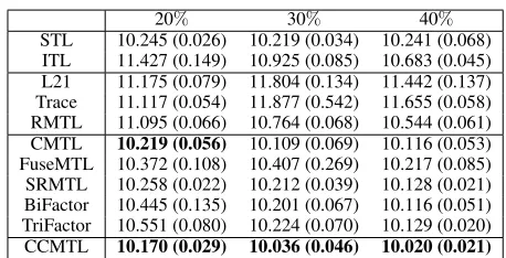
Table 5: Results (RMSE) on Schooldataset. The table re-ports the mean and standard errors over5random runs. The best model and the statistical competitive models (by paired

t-testwithα= 0.05) are shown in bold.

20% 30% 40%

STL 10.245 (0.026) 10.219 (0.034) 10.241 (0.068) ITL 11.427 (0.149) 10.925 (0.085) 10.683 (0.045) L21 11.175 (0.079) 11.804 (0.134) 11.442 (0.137) Trace 11.117 (0.054) 11.877 (0.542) 11.655 (0.058) RMTL 11.095 (0.066) 10.764 (0.068) 10.544 (0.061) CMTL 10.219 (0.056) 10.109 (0.069) 10.116 (0.053) FuseMTL 10.372 (0.108) 10.407 (0.269) 10.217 (0.085) SRMTL 10.258 (0.022) 10.212 (0.039) 10.128 (0.021) BiFactor 10.445 (0.135) 10.201 (0.067) 10.116 (0.051) TriFactor 10.551 (0.080) 10.224 (0.070) 10.129 (0.020) CCMTL 10.170 (0.029) 10.036 (0.046) 10.020 (0.021)

values for the problem (2). Whenλtakes larger values (>1), the objective values of ADMM method tend to monoton-ically increase, reflecting the increasing importance of the regularization term, but with a smaller slope for our solvers compared to the ADMM-based one. In addition to the lower objective function, our solver is clearly more computation-ally efficient than the expensive ADMM-based solver. The proposed solver shows stability in runtime, by taking at max-imum two seconds for all possibleλvalues, compared to a runtime in the range of[605−5760]seconds for the ADMM-based solver, on theSchooldata.

Comparison with SoA MTL methods. CCMTL is com-pared with the state-of-the-art methods in terms of the Root Mean Squared Error (RMSE). All experiments are repeated 5 times with different shuffling. In all result’s tables, we compare the best performing method with the remaining ones using the paired t-test (with α = 0.05). The best method and the methods that cannot be statistically outper-formed (by the best one) are shown in boldface.

Table 6: Results (RMSE and runtime) on Retail datasets. The table reports the mean and standard errors over 5 random runs. The best model and the statistical competitive models (by pairedt-testwithα= 0.05) are shown in bold. The best runtime for MTL methods is shown in boldface.

Sales Ta-Feng

RMSE Time(s) RMSE Time(s)

STL 2.861 (0.02) 0.1 0.791 (0.01) 0.2

ITL 3.115 (0.02) 0.1 0.818 (0.01) 0.4

L21 3.301 (0.01) 11.8 0.863 (0.01) 831.2 Trace 3.285 (0.21) 10.4 0.863 (0.01) 582.3 RMTL 3.111 (0.01) 3.4 0.833 (0.01) 181.5

CMTL 3.088 (0.01) 43.4 - >24h

FuseMTL 2.898 (0.01) 4.3 0.764 (0.01) 8483.3

SRMTL 2.854 (0.02) 10.3 - >24h

BiFactor 2.882 (0.01) 55.7 - >24h

TriFactor 2.857 (0.04) 499.1 - >24h

CCMTL 2.793 (0.01) 1.8 0.767 (0.01) 35.3

better than all SoA methods, except for the BiFactor which performs as well as CCMTL on theSyndataset.

The results on theSchooldataset are depicted in Table 5 with a ratio of training samples ranging from20%to40%. It appears to be that, unlike theSyndata, theSchooldata has tasks that are rather homogeneous, therefore, ITL performs the worst and STL shows its superiority on many of the MTL methods (L21, Trace, RMTL, FuseMTL and SRMTL). MT-Factor and TriMT-Factor outperform STL only when the train-ing ratio is larger than30%and40%, respectively. CCMTL, again, performs better than all competitive methods, on all training rations; CCMTL is also statistically the best per-forming method, expect for CMTL (with ratio20%) where the null hypothesis could not be rejected.

Table 6 depicts the results on two retail datasets:Sales andTa-Feng; it also depicts the time required (in seconds) for the training using the best found parametrization for each method. Here50%of samples are used for training. The best runtime for MTL methods is shown in boldface. Tasks in these two datasets are, again, rather homogeneous, therefore, the baseline STL has a competitive performance and out-performs many MTL methods. STL outout-performs ITL, L21, Trace3_{, RMTL, CMTL, FuseMTL, SRMTL, BiFactor, and}

TriFactor on the Salesdataset, and outperforms ITL, L21, Trace and RMTL on theTa-Fengdata4_{. CCMTL is the only}

method that performs better (also statistically better) than STL on both data sets; it also outperforms all MTL meth-ods (with statistical significance) on both data sets, except for FuseMTL which performs slightly better than CCMTL only on the Ta-Feng data. CCMTL requires the smallest runtime in comparison with the competitor MTL algorithms. OnTa-Fengdataset, CCMTL requires only around30 sec-onds, while the SoA methods need up to hours or even days. Table 7 depicts the results on the Transportation

3

The hyperparameters searching range for L21 and Trace are shifted to[100_,1010_]

forTa-Fengdataset to get reasonable results.

4

We set a timeout at24h. CMTL, SRMTL, BiFactor, and Tri-Factor did not return the result on this timeout for theTa-Feng dataset.

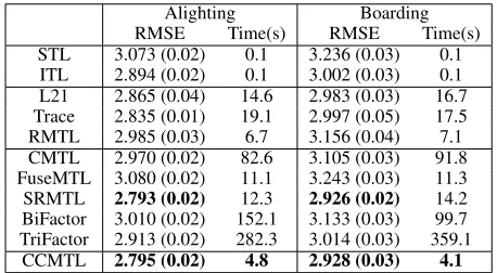
Table 7: Results (RMSE and runtime) on Transportation datasets. The table reports the mean and standard errors over 5random runs. The best model and the statistical competi-tive models (by pairedt-testwithα = 0.05) are shown in bold. The best runtime for MTL methods is shown in bold-face.

Alighting Boarding

RMSE Time(s) RMSE Time(s)

STL 3.073 (0.02) 0.1 3.236 (0.03) 0.1

ITL 2.894 (0.02) 0.1 3.002 (0.03) 0.1

L21 2.865 (0.04) 14.6 2.983 (0.03) 16.7 Trace 2.835 (0.01) 19.1 2.997 (0.05) 17.5

RMTL 2.985 (0.03) 6.7 3.156 (0.04) 7.1

CMTL 2.970 (0.02) 82.6 3.105 (0.03) 91.8 FuseMTL 3.080 (0.02) 11.1 3.243 (0.03) 11.3 SRMTL 2.793 (0.02) 12.3 2.926 (0.02) 14.2 BiFactor 3.010 (0.02) 152.1 3.133 (0.03) 99.7 TriFactor 2.913 (0.02) 282.3 3.014 (0.03) 359.1

CCMTL 2.795 (0.02) 4.8 2.928 (0.03) 4.1

datasets, using two different target attributes (alighting and boarding); again, the runtime is presented for the best-found parametrization, and the best runtime achieved by the MTL methods are shown in boldface. The results on this dataset are interesting, especially because both base-lines are not competitive as in the previous datasets. This could, safely, lead to the conclusion that the tasks belong to latent groups, where tasks are homogeneous intra-group, and heterogeneous inter-groups. All MTL methods (except the FuseMTL) outperform at least one of the baselines (STL and ITL) on both datasets. Our approach, CCMTL, seems to reach the right balance between task independence (ITL) and complete correlation (STL), as confirmed by the results; it achieves, statistically, the lowest RMSE against the base-lines and the all other MTL methods (except SRMTL), and it is at least 40% faster than the fastest MTL method (RMTL).

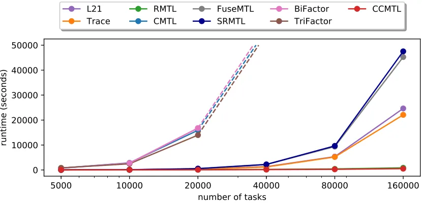
Scalability. In the scalability analysis, we use the ScaleSyndataset. We search the hyperparameters for all the methods on the smallest one with5ktasks and evaluate the runtime of the best-found hyperparameters on all the oth-ers. Figure 1 shows the recorded runtime in seconds while presenting the number of tasks in the log-scale. As can be seen, CMTL, MTFactor, and TriFactor were not capable to process 40k tasks in less than 24 hours, therefore, they were stopped (the extrapolation for the minimum needed runtime can be seen as a dashed line). FuseMTL, SRMTL, L21, and Trace tend to show a super-linear growth of the needed run-time in the log-scale. Both CCMTL and RMTL show con-stant behavior in the number of tasks, where only around 500 and800seconds are needed for the dataset with160k

5000

10000

20000

40000

80000

160000

number of tasks

0

10000

20000

30000

40000

50000

runtime (seconds)

L21

Trace

RMTL

CMTL

FuseMTL

SRMTL

BiFactor

TriFactor

CCMTL

Figure 1: Scalability experiments on synthetic datasets with increasing number of tasks (log scale on task number)

Related Work

Zhang and Yang (Zhang and Yang 2017), in their survey, classify multi-task learning into different categories: fea-ture learning, low-rank approaches, and task clustering ap-proaches, among others. These categories are characterized mainly by how the information between the different tasks is shared and which information is subject to sharing.

One type of MTL perform joint feature learning (L21) that assumes all tasks share a common set of features and penal-izes it by`2,1-norm regularization (Argyriou, Evgeniou, and Pontil 2007; 2008; Liu, Ji, and Ye 2009). Another way to capture the task relationship is to constrain the models from different tasks to share a low-dimensional subspace, i.e.W

is of low-rank (Trace) (Ji and Ye 2009). Both L21 and Trace assumes all the tasks are relevant, which is usually not true in real-world applications. Chen et al. (Chen, Zhou, and Ye 2011) propose robust multi-task learning (RMTL) in identi-fying irrelevant tasks by integrating the low-rank and group-sparse structures. These methods are relatively fast but can-not capture the task relationship when they belong to differ-ent latdiffer-ent groups.

The task clustering approaches aim at solving this issue where different tasks form clusters of similar tasks. Jacob et al. (Jacob, Vert, and Bach 2009) propose to integrate the ob-jective of k-means into the learning framework and solve a relaxed convex problem. Zhou et al. (Zhou, Chen, and Ye 2011a) use a similar idea for task clustering, but with a different optimization method. Zhou and Zhao (Zhou and Zhao 2016) propose to cluster tasks by identifying represen-tative tasks. Another way of performing task clustering is through the decomposition of the weight matrixW (Kumar and Daume III 2012; Barzilai and Crammer 2015). Later, a similar idea is performed with co-clustering of the features and the tasks (Murugesan, Carbonell, and Yang 2017). De-spite being effective, these methods are expensive to train and the number of clusters is needed as a hyperparameter

which makes the model tuning even more difficult.

Fused Multi-task Learning (FuseMTL) (Zhou et al. 2012; Chen et al. 2010) and Graph regularized Multi-task Learn-ing (SRMTL) (Zhou, Chen, and Ye 2011b) are the most related works, where `1 norm and squared `2 is used as the regularizer. As shown in the experiments, with`2norm CCMTL outperforms FuseMTL and SRMTL in most cases. In addition, the underlying optimization method is also dif-ferent, where the proposed CCMTL runs much faster. An-other closely related work is a multi-level clustering method (Han and Zhang 2015), where objective function also usesl2 norm. It looks similar to the proposed one if only one layer is considered (Zhang and Yang 2017). However, the method scales quadratically since constraint is on all the pairs of tasks, making it unsuitable for the studied problem in this paper with a massive number of tasks.

Conclusion

In this paper, we study the multi-task learning problem with a massive number of tasks. We integrate convex clustering

into the multi-task regression learning problem that captures tasks’ relationships on the k-NN graph of the prediction models. Further, we present an approach CCMTL that solves this problem efficiently and is guaranteed to converge to the global optimum. Extensive experiments show that CCMTL makes a more accurate prediction, runs faster than SoA com-petitors on both synthetic and real-world datasets, and scales linearly in the number of tasks. CCMTL will serve as a method for a wide range of large-scale regression applica-tions where the number of tasks is tremendous. In the future, we will explore the use of the proposed method for online learning and high-dimensional problem.

Acknowledgments

helpful comments and Prof. Yiannis Koutis for sharing the implementation of CMG.

References

Argyriou, A.; Evgeniou, T.; and Pontil, M. 2007. Multi-task feature learning. InNIPS, 41–48.

Argyriou, A.; Evgeniou, T.; and Pontil, M. 2008. Convex multi-task feature learning. Machine Learning73(3):243– 272.

Bakker, B., and Heskes, T. 2003. Task clustering and gating for bayesian multitask learning. Journal of Machine Learn-ing Research4(May):83–99.

Barzilai, A., and Crammer, K. 2015. Convex multi-task learning by clustering. InArtificial Intelligence and Statis-tics, 65–73.

Beck, A. 2015. On the convergence of alternating minimiza-tion for convex programming with applicaminimiza-tions to iteratively reweighted least squares and decomposition schemes.SIAM Journal on Optimization25(1):185–209.

Chen, X.; Kim, S.; Lin, Q.; Carbonell, J. G.; and Xing, E. P. 2010. Graph-structured multi-task regression and an effi-cient optimization method for general fused lasso. arXiv preprint arXiv:1005.3579.

Chen, J.; Zhou, J.; and Ye, J. 2011. Integrating low-rank and group-sparse structures for robust multi-task learning. InKDD, 42–50. ACM.

Chi, E. C., and Lange, K. 2015. Splitting methods for convex clustering. Journal of Computational and Graphical Statis-tics24(4):994–1013.

Cohen, M.; Kyng, R.; Miller, G.; Pachocki, J.; Peng, R.; Rao, A.; and Xu, S. 2014. Solving sdd linear systems in nearly m log 1/2 n time. InSTOC, 343–352. ACM.

Deng, D.; Shahabi, C.; Demiryurek, U.; and Zhu, L. 2017. Situation aware multi-task learning for traffic prediction. In

ICDM, 81–90. IEEE.

Dheeru, D., and Karra Taniskidou, E. 2017. UCI machine learning repository.

Hallac, D.; Leskovec, J.; and Boyd, S. 2015. Network lasso: Clustering and optimization in large graphs. InKDD, 387– 396. ACM.

Han, L., and Zhang, Y. 2015. Learning multi-level task groups in multi-task learning. InAAAI, volume 15, 2638– 2644.

He, X., and Moreira-Matias, L. 2018. Robust continuous co-clustering.arXiv preprint arXiv:1802.05036.

Hocking, T.; Joulin, A.; Bach, F.; and Vert, J. 2011. Cluster-path an algorithm for clustering using convex fusion penal-ties. InICML.

Ioannis, K.; Miller, G.; and Tolliver, D. 2011. Combinatorial preconditioners and multilevel solvers for problems in com-puter vision and image processing. Computer Vision and Image Understanding115(12):1638 – 1646.

Jacob, L.; Vert, J.-p.; and Bach, F. R. 2009. Clustered multi-task learning: A convex formulation. InNIPS, 745–752.

Ji, S., and Ye, J. 2009. An accelerated gradient method for trace norm minimization. InICML, 457–464. ACM. Kelner, J.; Orecchia, L.; Sidford, A.; and Zhu, Z. 2013. A simple, combinatorial algorithm for solving sdd systems in nearly-linear time. InSTOC, 911–920. ACM.

Kumar, A., and Daume III, H. 2012. Learning task grouping and overlap in multi-task learning.ICML.

Li, L.; He, X.; and Borgwardt, K. 2018. Multi-target drug repositioning by bipartite block-wise sparse multi-task learning.BMC systems biology12(4):55.

Liu, J.; Ji, S.; and Ye, J. 2009. Multi-task feature learning via efficient l 2, 1-norm minimization. InUAI, 339–348. AUAI Press.

Murugesan, K.; Carbonell, J.; and Yang, Y. 2017. Co-clustering for multitask learning. ICML.

Shah, S. A., and Koltun, V. 2017. Robust continuous clus-tering. Proceedings of the National Academy of Sciences

114(37):9814–9819.

Tan, S. C., and San Lau, J. P. 2014. Time series cluster-ing: A superior alternative for market basket analysis. In

Proceedings of the First International Conference on Ad-vanced Data and Information Engineering (DaEng-2013), 241–248. Springer, Singapore.

Wang, Q.; Gong, P.; Chang, S.; Huang, T. S.; and Zhou, J. 2016. Robust convex clustering analysis. InICDM, 1263– 1268. IEEE.

Zhang, Y., and Yang, Q. 2017. A survey on multi-task learn-ing.arXiv preprint arXiv:1707.08114v2.

Zhang, Y., and Yeung, D.-Y. 2014. A regularization ap-proach to learning task relationships in multitask learn-ing.ACM Transactions on Knowledge Discovery from Data (TKDD)8(3):12.

Zhou, Q., and Zhao, Q. 2016. Flexible clustered multi-task learning by learning representative multi-tasks. IEEE Trans. Pattern Anal. Mach. Intell.38(2):266–278.

Zhou, J.; Liu, J.; Narayan, V. A.; and Ye, J. 2012. Modeling disease progression via fused sparse group lasso. InKDD, 1095–1103. ACM.

Zhou, J.; Chen, J.; and Ye, J. 2011a. Clustered multi-task learning via alternating structure optimization. In NIPS, 702–710.