The Thirty-Third AAAI Conference on Artificial Intelligence (AAAI-19)
Fully Convolutional Network with
Multi-Step Reinforcement Learning for Image Processing
Ryosuke Furuta, Naoto Inoue, Toshihiko Yamasaki
Department of Information and Communication Engineering, The University of Tokyo, Tokyo, Japan {furuta, inoue, yamasaki}@hal.t.u-tokyo.ac.jp
Abstract
This paper tackles a new problem setting: reinforcement learning with pixel-wise rewards (pixelRL) for image pro-cessing. After the introduction of the deep Q-network, deep RL has been achieving great success. However, the applica-tions of deep RL for image processing are still limited. There-fore, we extend deep RL to pixelRL for various image pro-cessing applications. In pixelRL, each pixel has an agent, and the agent changes the pixel value by taking an action. We also propose an effective learning method for pixelRL that signifi-cantly improves the performance by considering not only the future states of the own pixel but also those of the neighbor pixels. The proposed method can be applied to some image processing tasks that require pixel-wise manipulations, where deep RL has never been applied.
We apply the proposed method to three image processing tasks: image denoising, image restoration, and local color enhancement. Our experimental results demonstrate that the proposed method achieves comparable or better performance, compared with the state-of-the-art methods based on super-vised learning.
Introduction
After the introduction of the deep Q-network (DQN) (Mnih et al. 2013), which can play Atari games on the human level, much attention has been focused on deep reinforce-ment learning (RL). Recently, deep RL is also applied to a variety of image processing tasks (Li et al. 2018; Lan et al. 2018; Park et al. 2018). However, these methods can execute only global actions for the entire image and are limited to simple applications, e.g., image cropping (Li et al. 2018) and global color enhancement (Park et al. 2018; Hu et al. 2018). Therefore, these methods cannot be applied to applications that require pixel-wise manipulations such as image denoising.
To overcome this drawback, we propose a new problem setting: pixelRL for image processing. PixelRL is a multi-agent RL problem, where the number of multi-agents is equal to that of pixels. The agents learn the optimal behavior to max-imize the mean of the expected total rewards at all pixels. Each pixel value is regarded as the current state and is iter-atively updated by the agent’s action. Applying the existing
Copyright c2019, Association for the Advancement of Artificial Intelligence (www.aaai.org). All rights reserved.
techniques of the multi-agent RL to pixelRL is impractical in terms of computational cost because the number of agents is extremely large. Therefore, we solve the problem by em-ploying the fully convolutional network (FCN). The merit of using FCN is that all the agents can share the parameters and learn efficiently. Herein, we also proposereward map convolution, which is an effective learning method for pix-elRL. By the proposed reward map convolution, each agent considers not only the future states of its own pixel but also those of the neighbor pixels.
The proposed pixelRL is applied to image denoising, im-age restoration, and local color enhancement. To the best of our knowledge, this is the first work to apply RL to such low-level image processing for each pixel or each local re-gion. Our experimental results show that the agents trained with the pixelRL and the proposed reward map convolution achieve comparable or better performance, compared with state-of-the-art methods based on supervised learning. Al-though the actions must be pre-defined for each application, the proposed method is interpretable by observing the ac-tions executed by the agents, which is a novel and different point from the existing deep learning-based image process-ing methods for such applications.
Our contributions are summarized as follows:
• We propose a novel problem setting: pixelRL for image processing, where the existing techniques for multi-agents RL cannot be applied.
• We proposereward map convolution, which is an effective learning method for pixelRL and boosts the performance.
• We apply the pixelRL to image denoising, image restora-tion, and local color enhancement. The proposed method is a completely novel approach for these tasks, and shows better or comparable performance, compared with state-of-the-art methods.
• The actions executed by the agents are interpretable to humans, which is of great difference from conventional CNNs.
Related Works
Deep RL for image processing
super-resolution method for face images. The agent first chooses a local region and inputs it to the local enhancement net-work. The enhancement network converts the local patch to a high-resolution one, and the agents chooses the next local patch that should be enhanced. This process is repeated un-til the maximum time step; consequently, the entire image is enhanced. Li et al. (2018) used deep RL for image crop-ping. The agent iteratively reshapes the cropping window to maximize the aesthetics score of the cropped image. Yu et al. (2018) proposed the RL-restore method, where the agent selects a toolchain from a toolbox (a set of light-weight CNNs) to restore a corrupted image. Park et al. (2018) pro-posed a color enhancement method using DQN. The agent iteratively chooses the image manipulation action (e.g., in-crease brightness) and retouches the input image. The ward is defined as the negative distance between the re-touched image by the agent and the one by an expert. A similar idea is proposed by Hu et al. (2018), where the agent retouches from RAW images. As discussed in the introduc-tion, all the above methods execute global actions for entire images. In contrast, we tackle pixelRL, where pixel-wise ac-tions can be executed.
Wulfmeier et al. (2015) used the FCN to solve the inverse reinforcement learning problem. This problem setting is dif-ferent from ours because one pixel corresponds to one state, and the number of agents is one in their setting. In contrast, our pixelRL has one agent at each pixel.
Image Denoising
Image denoising methods are classified into two categories: non-learning and learning based. Many classical methods are categorized into the former class (e.g., BM3D (Dabov et al. 2007)). Although learning-based methods include dictionary-based methods such as (Mairal et al. 2009), the recent trends in image denoising is neural network-based methods (Zhang et al. 2017; Lefkimmiatis 2017). Gener-ally, neural-network-based methods have shown better per-formances, compared with non-leaning-based methods.
Our denoising method based on pixelRL is a completely different approach from other neural network-based meth-ods. While most of neural-network-based methods learn to regress noise or true pixel values from a noisy input, our method iteratively removes noise with the sequence of sim-ple pixel-wise actions (basic filters).
Image Restoration
Similar to image denoising, image restoration (also called image inpainting) methods are divided into non-learning and learning-based methods. In the former methods such as (Bertalmio et al. 2000), the target blank regions are filled by propagating the pixel values or gradient informa-tion around the regions. The filling process is highly sophis-ticated, but they are based on a handcrafted-algorithm. Roth and Black (2005) proposed a Markov random field-based model to learn the image prior to the neighbor pixels. Mairal et al. (2008) proposed a learning-based method that creates a dictionary from an image database using K-SVD, and ap-plied it to image denoising and inpainting. Recently, deep-neural-network-based methods were proposed (Xie, Xu, and
Chen 2012; Liu, Pan, and Su 2017), and the U-Net-based in-painting method (Liu, Pan, and Su 2017) showed much bet-ter performance than other methods.
Our method is categorized into the learning-based method because we used training images to optimize the policies. However, similar to the classical inpainting methods, our method successfully propagates the neighbor pixel values with the sequence of basic filters.
Color Enhancement
One of the classical methods is color transfer proposed by Reinhard et al. (2001), where the global color distribution of the reference image is transfered to the target image. Hwang et al. (2012) proposed an automatic local color en-hancement method based on image retrieval. This method enhances the color of each pixel based on the retrieved im-ages with smoothness regularization, which is formulated as a Gaussian MRF optimization problem.
Yan et al. (2016) proposed the first color enhancement method based on deep learning. They used a DNN to learn a mapping function from the carefully designed pixel-wise features to the desired pixel values. Gharbi et al. (2017) used a CNN as a trainable bilateral filter for high-resolution im-ages and applied it to some image processing tasks. Simi-larly, for fast image processing, Chen et al. (2017) adopted an FCN to learn an approximate mapping from the input to the desired images. Unlike deep learning-based methods that learn the input for an output mapping, our color enhance-ment method is interpretable because our method enhances each pixel value iteratively with actions such as (Park et al. 2018; Hu et al. 2018).
Background Knowledge
Herein, we extend the asynchronous advantage actor-critic (A3C) (Mnih et al. 2016) for the pixelRL problem because A3C showed good performance with efficient training in the original paper1. In this section, we briefly review the training algorithm of A3C. A3C is one of the actor-critic methods, which has two networks: policy network and value network. We denote the parameters of each network asθpandθv, re-spectively. Both networks use the current state s(t) as the input, wheres(t) is the state at time stept. The value net-work outputs the value V(s(t)): the expected total rewards from states(t), which shows how good the current state is.
The gradient forθvis computed as follows:
R(t)=r(t)+γr(t+1)+γ2r(t+2)+· · ·
+γn−1r(t+n−1)+γnV(s(t+n)), (1)
dθv=∇θv
R(t)−V(s(t))
2
, (2)
whereγiis thei-th power of the discount factorγ.
The policy network outputs the policyπ(a(t)|s(t))
(prob-ability through softmax) of taking actiona(t) ∈ A. There-fore, the output dimension of the policy network is|A|. The
1
gradient forθpis computed as follows:
A(a(t), s(t)) = R(t)−V(s(t)), (3)
dθp = −∇θplogπ(a
(t)|s(t))A(a(t), s(t)).(4)
A(a(t), s(t)) is called the advantage, and V(s(t)) is
sub-tracted in Eq. (3) to reduce the variance of the gradient. For more details, see (Mnih et al. 2016).
Reinforcement Learning with Pixel-wise
Rewards (PixelRL)
Here, we describe the proposed pixelRL problem setting. LetIibe thei-th pixel in the input imageIthat hasN pix-els(i= 1,· · · , N). Each pixel has an agent, and its policy is denoted asπi(a(it)|s(it)), wherea(it)(∈ A)ands(it)are the action and the state of thei-th agent at time stept, respec-tively. Ais the pre-defined action set, ands(0)i = Ii. The agents obtain the next statess(t+1) = (s(t+1)
1 ,· · · , s (t+1)
N )
and rewardsr(t) = (r1(t),· · ·, rN(t)) from the environment by taking the actions a(t) = (a(t)
1 ,· · · , a (t)
N ). The
objec-tive of the pixelRL problem is to learn the optimal policies π = (π1,· · · , πN)that maximize the mean of the total
ex-pected rewards at all pixels:
π∗ = argmax
π
Eπ
∞
X
t=0
γtr(t)
!
, (5)
r(t) = 1
N N
X
i=1
r(it), (6)
wherer(t)is the mean of the rewardsr(it)at all pixels. A naive solution for this problem is to train a network that output Q-values or policies for all possible set of actions a(t). However, it is computationally impractical because the
dimension of the last fully connected layer must be|A|N,
which is too large.
Another solution is to divide this problem intoN inde-pendent subproblems and trainNnetworks, where we train thei-th agent to maximize the expected total reward at the
i-th pixel:
π∗i = argmax
πi
Eπi
∞
X
t=0
γtr(it)
!
. (7)
However, trainingN networks is also computationally im-practical when the number of pixels is large. In addition, it treats only the fixed size of images. To solve the problems, we employ a FCN instead ofNnetworks. By using the FCN, all theNagents can share the parameters, and we can paral-lelize the computation ofNagents on a GPU, which renders the training efficient. Herein, we employ A3C and extend it to the fully convolutional form. Our architecture is illus-trated in the supplemental material.
The pixelRL setting is different from typical multi-agent RL problems in terms of two points. The first point is that the number of agentsN is extremely large (>105). Therefore,
typical multi-agent learning techniques such as (Lowe et al.
2017) cannot be directly applied to the pixelRL. Next, the agents are arrayed in a 2D image plane. In the next section, we propose an effective learning method that boosts the per-formance of the pixelRL agents by leveraging this property, namedreward map convolution.
Reward Map Convolution
Here, for the ease of understanding, we first consider the one-step learning case (i.e.,n= 1in Eq. (1)).
When the receptive fields of the FCNs are 1x1 (i.e., all the convolution filters in the policy and value network are 1x1), theNsubproblems are completely independent. In that case, similar to the original A3C, the gradient of the two networks are computed as follows:
R(it) = ri(t)+γV(s(it+1)), (8)
dθv = ∇θv
1
N N
X
i=1
R(it)−V(s(it))
2
, (9)
A(a(it), s(it)) = Ri(t)−V(s(it)), (10)
dθp=−∇θp
1
N N
X
i=1
logπ(a(it)|s(it))A(a(it), s(it)). (11)
As shown in Eqs. (9) and (11), the gradient for each network parameter is the average of the gradients at all pixels.
However, one of the recent trends in CNNs is to enlarge the receptive field to boost the network performance (Yu, Koltun, and Funkhouser 2017; Zhang et al. 2017). Our net-work architecture, which was inspired by (Zhang et al. 2017) in the supplemental material, has a large receptive field. In this case, the policy and value networks observe not only the
i-th pixels(it)but also the neighbor pixels to output the pol-icyπand valueV at thei-th pixel. In other words, the action
a(it)affects not only thes(it+1)but also the policies and val-ues inN(i)at the next time step, whereN(i)is the local window centered at thei-th pixel. Therefore, to consider it, we replaceRiin Eq. (8) as follows:
R(it)=ri(t)+γ X
j∈N(i)
wi−jV(s
(t+1)
j ), (12)
wherewi−jis the weight that means how much we consider
the values V of the neighbor pixels at the next time step (t+ 1).wcan be regarded as a convolution filter weight and can be learned simultaneously with the network parameters
θpandθv. It is noteworthy that the second term in Eq. (12) is a 2D convolution because each pixelihas a 2D coordinate (ix, iy).
Using the matrix form, we can define theR(t) in then
-step case.
R(t)=r(t)+γw∗r(t+1)+γ2w2∗r(t+2)+· · ·
+γn−1wn−1∗r(t+n−1)+γnwn∗V(s(t+n)), (13)
Table 1: Actions for image denoising and restoration.
action filter size parameter
1 box filter 5x5
-2 bilateral filter 5x5 σc= 1.0, σS= 5.0
3 bilateral filter 5x5 σc= 0.1, σS= 5.0
4 median filter 5x5
-5 Gaussian filter 5x5 σ= 1.5
6 Gaussian filter 5x5 σ= 0.5
7 pixel value += 1 -
-8 pixel value -= 1 -
-9 do nothing -
-θv in Eqs. (9) and (11), the gradient forw is computed as follows:
dw=−∇w1
N N
X
i=1
logπ(a(it)|s(it))(R(it)−V(s(it)))
+∇w1
N N
X
i=1
(R(it)−V(s(it)))2. (14)
Similar to typical policy gradient algorithms, the first term in Eq. (14) encourages a higher expected total reward. The second term operates as a regularizer such thatRiis not de-viated from the predictionV(s(it))by the convolution.
Applications and Results
We implemented the proposed method on Python with Chainer (Tokui, Oono, and Hido 2015) and ChainerRL2 li-braries, and applied it to three different applications.
Image denoising
Method The input imageI(= s(0))is a noisy gray scale
image, and the agents iteratively remove the noises by ex-ecuting actions. It is noteworthy that the proposed method can also be applied to color images by independently ma-nipulating on the three channels. Table 1 shows the list of actions that the agents can execute, which were empirically decided. We defined the rewardri(t)as follows:
r(it)= (Iitarget−s(it))2−(Iitarget−s(it+1))2, (15)
whereIitarget is the i-th pixel value of the original clean image. Intuitively, Eq. (15) means how much the squared er-ror on thei-th pixel was decreased by the action a(it). As shown in (Maes, Denoyer, and Gallinari 2009), maximizing the total reward in Eq. (15) is equivalent to minimizing the squared error between the final states(tmax)and the original
clean imageItarget. We set the number of training episodes to 30,000 and the length of each episodetmaxto 5. We set the filter size ofwto33×33, which is equal to the receptive field size of the policy and value networks. The other imple-mentation details are shown in the supplemental material. We used BSD68 dataset (Roth and Black 2005), which has
2
https://github.com/chainer/chainerrl
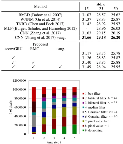
Table 2: PSNR [dB] on BSD68 test set with Gaussian noise.
Method std.σ
15 25 50
BM3D (Dabov et al. 2007) 31.07 28.57 25.62
WNNM (Gu et al. 2014) 31.37 28.83 25.87
TNRD (Chen and Pock 2017) 31.42 28.92 25.97 MLP (Burger, Schuler, and Harmeling 2012) - 28.96 26.03 CNN (Zhang et al. 2017) 31.63 29.15 26.19 CNN (Zhang et al. 2017) +aug. 31.66 29.18 26.20
Proposed
+convGRU +RMC +aug.
31.17 28.75 25.78
X 31.26 28.83 25.87
X X 31.40 28.85 25.88
X X X 31.49 28.94 25.95
0 2000000 4000000 6000000 8000000 10000000 12000000
1 2 3 4 5
# of
pix
el
s
time step t
1. box filter 2. bilateral filter 3. bilateral filter 4. median filter 5. Gaussian filter 6. Gaussian filter 7. pixel value += 1 8. pixel value -= 1 9. do nothing
𝜎𝑐= 1.0 𝜎𝑐= 0.1
𝜎 = 1.5 𝜎 = 0.5
Figure 1: Number of actions executed at each time step for Gaussian denoising (σ= 50) on the BSD68 test set.
428 train images and 68 test images. Similar to (Zhang et al. 2017), we added 4,774 images from Waterloo exploration database (Ma et al. 2017) to the training set.
Results Table 2 shows the comparison of Gaussian
de-noising with other methods. RMC is the abbreviation for re-ward map convolution. Aug. means the data augmentation for test images, where a single test image was augmented to eight images by a left-right flip and90◦,180◦, and270◦ rotations, similar to (Timofte et al. 2017). We observed that CNN (Zhang et al. 2017) is the best. However, the proposed method achieved the comparable results with other state-of-the-art methods. Adding the convGRU to the policy network improved the PSNR by approximately +0.1dB. The RMC significantly improved the PSNR when σ = 15, but im-proved little whenσ= 25and50. That is because the agents can obtain much reward by removing the noises at their own pixels rather than considering the neighbor pixels when the noises are strong. The augmentation for test images further boosted the performance. We report the CNN (Zhang et al. 2017) with the same augmentation for a fair comparison. Almost similar results were obtained on Poisson denoising, which are shown in the supplemental material.
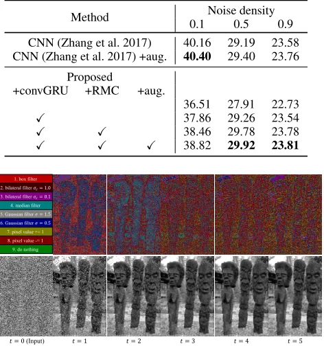
Table 3: PSNR [dB] on BSD68 test set with Salt&Pepper noise.
Method Noise density
0.1 0.5 0.9
CNN (Zhang et al. 2017) 40.16 29.19 23.58 CNN (Zhang et al. 2017) +aug. 40.40 29.40 23.76
Proposed
+convGRU +RMC +aug.
36.51 27.91 22.73
X 37.86 29.26 23.54
X X 38.46 29.78 23.78
X X X 38.82 29.92 23.81
1. box filter 2. bilateral filter 𝜎𝑐= 1.0
3. bilateral filter 𝜎𝑐= 0.1
4. median filter 5. Gaussian filter 𝜎 = 1.5
6. Gaussian filter 𝜎 = 0.5
7. pixel value += 1 8. pixel value -= 1 9. do nothing
𝑡 = 0(Input) 𝑡 = 1 𝑡 = 2 𝑡 = 3 𝑡 = 4 𝑡 = 5
Figure 2: Denoising process of the proposed method and the action map at each time step for salt and pepper denoising (density=0.9).
noises using strong filters (box filter, bilateral filterσc= 1.0, and Gaussian filterσ= 1.5); subsequently they adjusted the pixel values by the other actions (pixel values +=1 and -=1). Table 3 shows the comparison of salt and pepper de-noising. We observed that the RMC significantly improved the performance. In addition, the proposed method outper-formed the CNN (Zhang et al. 2017) when the noise density is 0.5 and 0.9. Unlike Gaussian and Poisson noises, it is dif-ficult to regress the noise with CNN when the noise density is high because the information of the original pixel value is lost (i.e., the pixel value was changed to 0 or 255 by the noise). In contrast, the proposed method can predict the true pixel values from the neighbor pixels with the iterative fil-tering actions.
We visualize the denoising process of the proposed method, and the action map at each time step in Fig. 2. We observed that the noises are iteratively removed by the cho-sen actions.
Fig. 3 shows the qualitative comparison with CNN (Zhang et al. 2017). The proposed method achieved both quantita-tive and visually better results for salt and pepper denoising.
Image Restoration
Method We applied the proposed method to “blind”
im-age restoration, where no mask of blank regions is provided. The proposed method iteratively inpaints the blank regions by executing actions. We used the same actions and reward
CNN
30.72 / 0.900 31.48Proposed/ 0.924 Ground truth
Input
Figure 3: Qualitative comparison of the proposed method and CNN (Zhang et al. 2017) for salt and pepper noise (den-sity=0.5). PSNR / SSIM are reported.
Table 4: Comparison on image restoration.
Method PSNR [dB] SSIM
Net-D and Net-E (Liu, Pan, and Su 2017) 29.53 0.846
CNN (Zhang et al. 2017) 29.75 0.858
Proposed
+convGRU +RMC
X 29.50 0.858
X X 29.97 0.868
function as those of image denoising, which are shown in Ta-ble 1 and Eq. (15), respectively.
For training, we used 428 training images from the BSD68 train set, 4,774 images from the Waterloo explo-ration database, and 20,122 images from the ILSVRC2015 val set (Russakovsky et al. 2015) (a total of 25,295 images). We also used 11,343 documents from the Newsgroups 20 train set (Lang 1995). During the training, we created each training image by randomly choosing an image from the 25,295 images and a document from 11,343 documents, and overlaid it on the image. The font size was randomly decided from the range [10,30]. The font type was randomly chosen betweenArialandTimes New Roman, where the bold and Italic options were randomly added. The intensity of the text region was randomly chosen from 0 or 255. We created the test set that has 68 images by overlaying the randomly cho-sen 68 documents from the Newsgroup 20 test set on the BSD68 test images. The settings of the font size and type were the same as those of the training. The random seed for the test set was fixed between the different methods. All the hyperparameters were same as those in image denoising, ex-cept for the length of the episodes, i.e.,tmax= 15.
Results Table 4 shows the comparison of the averaged
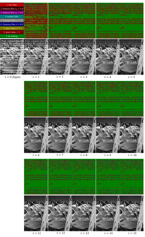
𝑡 = 0(Input) 𝑡 = 1 𝑡 = 2 𝑡 = 3 𝑡 = 4 𝑡 = 5
𝑡 = 6 𝑡 = 7 𝑡 = 8 𝑡 = 9 𝑡 = 10
𝑡 = 11 𝑡 = 12 𝑡 = 13 𝑡 = 14 𝑡 = 15 1. box filter
2. bilateral filter 𝜎𝑐= 1.0
3. bilateral filter 𝜎𝑐= 0.1
4. median filter 5. Gaussian filter 𝜎 = 1.5
6. Gaussian filter 𝜎 = 0.5
7. pixel value += 1 8. pixel value -= 1 9. do nothing
Figure 4: Restoration process of the proposed method and the action map at each time step.
similar reason to the case of the salt and pepper noise. Be-cause the information of the original pixel value is lost by the overlaid texts, its regression is difficult. In contrast, the proposed method predicts the true pixel value by iteratively propagating the neighbor pixel values with the filtering ac-tions.
Fig. 4 is the visualization of restoration process of the proposed method, and the action map at each time step. Fig. 5 shows the qualitative comparison with E and Net-D (Liu, Pan, and Su 2017) and CNN (Zhang et al. 2017). We observed that there are visually large differences between the results from the proposed method and those from the compared methods.
Local Color Enhancement
Method We also applied the proposed method to the
lo-cal color enhancement. We used the dataset created by (Yan et al. 2016), which has 70 train images and 45 test
im-CNN
28.05 / 0.852 28.92Proposed/ 0.881 Ground truth
Input Net-E and Net-D
28.25 / 0.851
Figure 5: Qualitative comparison of the proposed method with Net-E and Net-D (Liu, Pan, and Su 2017) and CNN (Zhang et al. 2017) on image restoration. PSNR / SSIM are reported.
Table 5: Thirteen actions for local color enhancement. Action
1 / 2 contrast ×0.95/×1.05
3 / 4 color saturation ×0.95/×1.05
5 / 6 brightness ×0.95/×1.05
7 / 8 red and green ×0.95/×1.05
9 / 10 green and blue ×0.95/×1.05
11 / 12 red and blue ×0.95/×1.05
13 do nothing
ages downloaded from Flicker. Using Photoshop, all the im-ages were enhanced by a professional photographer for three different stylistic local effects: Foreground Pop-Out, Local Xpro, and Watercolor. Inspired by (Park et al. 2018), we de-cided the action set as shown in Table 5. Given an input im-ageI, the proposed method changes the three channel pixel value at each pixel by executing an action. When inputting I to the network, the RGB color values were converted to CIELab color values. We defined the reward function as the decrease of L2 distance in the CIELab color space as fol-lows:
ri(t)=|Iitarget−si(t)|2− |Iitarget−s
(t+1)
i |2. (16)
All the hyperparameters and settings were same as those in image restoration, except for the length of episodes, i.e.,
tmax= 10.
Results Table 6 shows the comparison of mean L2 errors
on 45 test images. The proposed method achieved better re-sults than DNN (Yan et al. 2016) on all three enhancement styles, and comparable or slightly better results than pix2pix. We observed that the RMC improved the performance al-though their degrees of improvement depended on the styles. It is noteworthy that the existing color enhancement method using deep RL (Park et al. 2018; Hu et al. 2018) cannot be applied to this local enhancement application because they can execute only global actions.
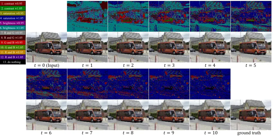
1. contrast ×0.95 2. contrast ×1.05 3. saturation ×0.95 4. saturation ×1.05 5. brightness ×0.95 6. brightness ×1.05 7. R and G ×0.95 8. R and G ×1.05 9. G and B ×0.95 10. G and B ×1.05 11. R and B ×0.95 12. R and B ×1.05 13. do nothing
𝑡 = 0(Input) 𝑡 = 1 𝑡 = 2 𝑡 = 3 𝑡 = 4 𝑡 = 5
𝑡 = 6 𝑡 = 7 𝑡 = 8 𝑡 = 9 𝑡 = 10 ground truth
Figure 6: Color enhancement process of the proposed method for watercolor, and the action map at each time step.
Table 6: Comparison of mean L2 testing errors on local color enhancement. The errors except for the proposed method and pix2pix are from (Yan et al. 2016).
Method Foreground Local Watercolor
Pop-Out Xpro
Original 13.86 19.71 15.30
Lasso 11.44 12.01 9.34
Random Forest 9.05 7.51 11.41
DNN (Yan et al. 2016) 7.08 7.43 7.20
Pix2pix (Isola et al. 2017) 5.85 6.56 8.84
Proposed
+convGRU +RMC
X 6.75 6.17 6.44
X X 6.69 5.67 6.41
Fig. 7 shows the qualitative comparison between the pro-posed method and DNN (Yan et al. 2016). The propro-posed method achieved both quantitatively and qualitatively better results.
Conclusions
We proposed a novel pixelRL problem setting and applied it to three different applications: image denoising, image restoration, and local color enhancement. We also proposed an effective learning method for the pixelRL problem, which boosts the performance of the pixelRL agents. Our ex-perimental results demonstrated that the proposed method achieved comparable or better results than state-of-the-art methods on each application. Different from the existing deep learning-based methods for such applications, the pro-posed method is interpretable. The interpretability of deep learning has been attracting much attention (Selvaraju et al. 2017), and it is especially important for some applications
DNN Proposed Ground truth
Input
Foreground Pop-Out
Local Xpro
Watercolor
Figure 7: Qualitative comparison of the proposed method and DNN (Yan et al. 2016). The saturation of the im-ages from DNN appear higher owning to the color correc-tion for the sRGB space (for details, see https://github.com/ stephenyan1231/dl-image-enhance).
such as medical image processing (Razzak, Naz, and Zaib 2018).
The proposed method can maximize the pixel-wise re-ward; in other words, it can minimize the pixel-wise non-differentiable objective function. Therefore, we believe that the proposed method can be potentially used for more image processing applications where supervised learning cannot be applied.
Acknowledgments
References
Bertalmio, M.; Sapiro, G.; Caselles, V.; and Ballester, C. 2000. Image inpainting. InSIGGRAPH.
Burger, H. C.; Schuler, C. J.; and Harmeling, S. 2012. Image denoising: Can plain neural networks compete with bm3d? InCVPR.
Cao, Q.; Lin, L.; Shi, Y.; Liang, X.; and Li, G. 2017. Attention-aware face hallucination via deep reinforcement learning. InCVPR.
Chen, Y., and Pock, T. 2017. Trainable nonlinear reaction diffusion: A flexible framework for fast and effective image restoration.IEEE TPAMI39(6):1256–1272.
Chen, Q.; Xu, J.; and Koltun, V. 2017. Fast image processing with fully-convolutional networks. InICCV.
Dabov, K.; Foi, A.; Katkovnik, V.; and Egiazarian, K. 2007. Image denoising by sparse 3-d transform-domain collabora-tive filtering.IEEE TIP16(8):2080–2095.
Gharbi, M.; Chen, J.; Barron, J. T.; Hasinoff, S. W.; and Du-rand, F. 2017. Deep bilateral learning for real-time im-age enhancement. ACM Transactions on Graphics (TOG)
36(4):118.
Gu, S.; Zhang, L.; Zuo, W.; and Feng, X. 2014. Weighted nuclear norm minimization with application to image de-noising. InCVPR.
Hu, Y.; He, H.; Xu, C.; Wang, B.; and Lin, S. 2018. Expo-sure: A white-box photo post-processing framework. ACM Transactions on Graphics (TOG)37(2):26.
Hwang, S. J.; Kapoor, A.; and Kang, S. B. 2012. Context-based automatic local image enhancement. InECCV. Isola, P.; Zhu, J.-Y.; Zhou, T.; and Efros, A. A. 2017. Image-to-image translation with conditional adversarial networks. InCVPR.
Lan, S.; Panda, R.; Zhu, Q.; and Roy-Chowdhury, A. K. 2018. Ffnet: Video fast-forwarding via reinforcement learn-ing. InCVPR.
Lang, K. 1995. Newsweeder: Learning to filter netnews. In
Machine Learning Proceedings. 331–339.
Lefkimmiatis, S. 2017. Non-local color image denoising with convolutional neural networks. InCVPR.
Li, D.; Wu, H.; Zhang, J.; and Huang, K. 2018. A2-rl: Aesthetics aware reinforcement learning for automatic im-age cropping. InCVPR.
Liu, Y.; Pan, J.; and Su, Z. 2017. Deep blind image inpaint-ing.CoRRabs/1712.09078.
Lowe, R.; Wu, Y.; Tamar, A.; Harb, J.; Abbeel, O. P.; and Mordatch, I. 2017. Multi-agent actor-critic for mixed cooperative-competitive environments. InNIPS.
Ma, K.; Duanmu, Z.; Wu, Q.; Wang, Z.; Yong, H.; Li, H.; and Zhang, L. 2017. Waterloo exploration database: New challenges for image quality assessment models. IEEE TIP
26(2):1004–1016.
Maes, F.; Denoyer, L.; and Gallinari, P. 2009. Structured prediction with reinforcement learning. Machine learning
77(2-3):271.
Mairal, J.; Bach, F.; Ponce, J.; Sapiro, G.; and Zisserman, A. 2009. Non-local sparse models for image restoration. In
ICCV.
Mairal, J.; Elad, M.; and Sapiro, G. 2008. Sparse represen-tation for color image restoration. IEEE TIP17(1):53–69. Mnih, V.; Kavukcuoglu, K.; Silver, D.; Graves, A.; Antonoglou, I.; Wierstra, D.; and Riedmiller, M. 2013. Play-ing atari with deep reinforcement learnPlay-ing. InNIPS Deep Learning Workshop.
Mnih, V.; Badia, A. P.; Mirza, M.; Graves, A.; Lillicrap, T.; Harley, T.; Silver, D.; and Kavukcuoglu, K. 2016. Asynchronous methods for deep reinforcement learning. In
ICML.
Park, J.; Lee, J.-Y.; Yoo, D.; and Kweon, I. S. 2018. Distort-and-recover: Color enhancement using deep reinforcement learning. InCVPR.
Razzak, M. I.; Naz, S.; and Zaib, A. 2018. Deep learning for medical image processing: Overview, challenges and the future. InClassification in BioApps. 323–350.
Reinhard, E.; Adhikhmin, M.; Gooch, B.; and Shirley, P. 2001. Color transfer between images. IEEE Computer graphics and applications21(5):34–41.
Roth, S., and Black, M. J. 2005. Fields of experts: A frame-work for learning image priors. InCVPR.
Russakovsky, O.; Deng, J.; Su, H.; Krause, J.; Satheesh, S.; Ma, S.; Huang, Z.; Karpathy, A.; Khosla, A.; Bernstein, M.; Berg, A. C.; and Fei-Fei, L. 2015. ImageNet Large Scale Visual Recognition Challenge. IJCV115(3):211–252. Selvaraju, R. R.; Cogswell, M.; Das, A.; Vedantam, R.; Parikh, D.; and Batra, D. 2017. Grad-cam: Visual expla-nations from deep networks via gradient-based localization. InICCV.
Timofte, R.; Agustsson, E.; Van Gool, L.; Yang, M.-H.; Zhang, L.; Lim, B.; Son, S.; Kim, H.; Nah, S.; Lee, K. M.; et al. 2017. Ntire 2017 challenge on single image super-resolution: Methods and results. InCVPR Workshop, 1110– 1121.
Tokui, S.; Oono, K.; and Hido, S. 2015. Chainer: a next-generation open source framework for deep learning. In
NIPS Workshop on Machine Learning Systems.
Wulfmeier, M.; Ondruska, P.; and Posner, I. 2015. Maxi-mum entropy deep inverse reinforcement learning. InNIPS Deep Reinforcement Learning Workshop.
Xie, J.; Xu, L.; and Chen, E. 2012. Image denoising and inpainting with deep neural networks. InNIPS.
Yan, Z.; Zhang, H.; Wang, B.; Paris, S.; and Yu, Y. 2016. Au-tomatic photo adjustment using deep neural networks.ACM Transactions on Graphics (TOG)35(2):11.
Yu, K.; Dong, C.; Lin, L.; and Loy, C. C. 2018. Crafting a toolchain for image restoration by deep reinforcement learn-ing. InCVPR.
Yu, F.; Koltun, V.; and Funkhouser, T. 2017. Dilated residual networks. InCVPR, 472–480.