A Toy Biological Modelling Through a Delayed Rational
Difference Equation
Adwitiya Chaudhuri
1& Sk. Sarif Hassan
21Department of Zoology 2Department of Mathematics
Pingla Thana Mahavidyalaya Maligram, Paschim Midnapur, 721140, India. Email: [email protected] & [email protected]
July 27, 2017
Abstract
In modelling of any biological systems, one of the important and fundamental issues is the depth of choice of detail. The relevance goes far beyond mathematical convenience to the heart of under-standing the mechanism, specifically, which details at one level are important to the determination of any phenomena at other levels and which can be ignored. The rational difference equations with delay surprisedly gained attention in modelling some of the complicated biological systems over last couple of decades. In this article, a (k+ 1)th order delayed rational difference equation
hn+1=
α+γhn−k
βhn+δhnhn−k+hn−k
, n= 0,1,2, . . .
is considered as a toy model and its behavior is investigated.
Keywords: Bio-System Modelling, Rational difference equation, Local asymptotic stability, Chaotic trajectory and Periodicity.
Mathematics Subject Classification: 39A10, 39A11
1
Introduction and Background
Nature is supernally complex! It is an authors perception that nature encourages people to explore her as closely as they wish but can never be touched. An apparently constant and stable system is often nothing but a balance of tendencies pushing the system towards different directions. The cumulative effect of various interactions and competing tendencies generally make it difficult to analyse the full picture at once. Mathematical language has been designed for precise description of dynamic process in biology. The rationale for constructing mathematical models of reality lies in simple formulas, for instance, that can relate the population of a species in a certain year to that of the following year. This strategy has enjoyed considerable success in natural sciences and there are growing literature exploring their usefulness. In most modern biology fields, it is important to know how populations grow and what factors influence their growth [1]. In this context, mathematical analysis indicates the consequences an equation might have, so that it can be checked against biological observation. Despite ecology knowl-edge of this kind is important in studies of bacterial growth, wildlife management and harvesting [2].
and increasingly attracts many mathematicians and non-mathematicians as well [5]. The basic ques-tions that arise in this regard are: how does one find an appropriate difference equation to model a situation? how does one understand the behaviour of the difference equation model once it has been formed? There is no scopes of confusion that the theory of difference equations will continue to play an important role in mathematics as a whole. It is found that a dynamic biological system may settle down into a particular pattern regardless of its initial values. The first few steps of iterations though may not really be indicative of what happens over long term. One of the significant biological conclusions from nonlinear models is that a population may exhibit cycles even when the environment is completely unchanging. Complicated behavior can be produced even by simple models. So the natural view that complicated population dynamics is the result of complex iterations and environment fluctuations would have to be abandoned. It is seen over decades, nonlinear difference equations of higher order with delay are of paramount importance in applications [6] & [7]. Such equations also appear naturally as discrete analogues and as numerical solutions of differential and delay differential equations which model various diverse phenomena in biology, ecology, physiology, physics, engineering and economics as said earlier. For greater detail of dynamics in biological systems one may refer to the books [8] & [9] and articles [10] & [11] .
In this article, a computational attempt without any rigorous theoretical exercise is made to explore the behavior of such a model which is commonly known asrational difference equation. We shall show how the dynamical behavior of a simple difference equation goes from a fixed point, through a sequence of bifurcations, into stable periodic cycles and finally into a regime of apparent chaos. This is illustrated with a particular example of a rational difference equation as stated below, but the emphasis is on the generic character of the process.
Consider the equation
hn+1=
α+γhn−k βhn+δhnhn−k+hn−k
, n= 0,1,2, . . . (1) where the parameterα, γ, B andD and the initial conditionsh−k, h−k+1. . . h0 are arbitrary real
num-bers.
The second order rational difference equation Eq.(1) with (k= 2) is studied when the parameters and the initial conditions are non-negative real numbers byY. Kostrov and Z. Kudlak in []. Here we proceed to comprehend the dynamics of the generalized Eq.(1) with delay k.
Before we proceed further here we review a very basic necessary results related to local stability of fixed points.
Definition 1: A difference equation of order (k+ 1) is of the form
zn+1=f(zn, zn−1, . . . , zn−k), n= 0,1,2, . . . (2)
where f is a continuous function which maps a subsetDk+1 into DandD⊂R. A fixed point ¯z of the
difference equation Eq. (2) is a point that satisfy the condition ¯z=f(¯z,z, . . . ,¯ z¯).
Definition 2: Let ¯zbe a fixed point of the Eq.(2), then ¯zislocally asymptotically stable if for every
this property.
Definition 4: An open ballB(a, r)∈Cis called aninvariant open ballof Eq.(2) ifz−k, . . . , z−1, z0∈ B(a, r) thenzn∈B(a, r) for alln >0. That is every solution of Eq.(2) with initial conditions inB(a, r) remains inB(a, r).
Definition 5: The difference equation Eq.(2) is said to bepermanent and bounded if there exist pos-itive real numbersM andN with 0< M ≤N <∞such that for any initial conditionsz−k, . . . , z−1, z0
there exists a positive integer P which depends on the initial conditions such thatM ≤ |zn| ≤N for all
n≥P.
The linearized equation associated with Eq.(2) about the equilibrium point ¯zis
yn+1= k
X
i=0
∂f(¯z,¯z, . . . ,z¯)
∂ui
yn−i
Its characteristic equation is
λk+1=
k
X
i=0
∂f(¯z,z, . . . ,¯ z¯)
∂ui
λn−i
wheren= 0,1,2, . . ..
Theorem 1.1. Assume that f is a C1-function and letz¯ a fixed point of Eq.(2). Then the following statements are true:
• If all the roots of the characteristic equation lie in the open unit disk|λ|<1, then the fixed point
¯
z of Eq.(2) is locally asymptotically stable.
• If at least one root of the characteristic equation has the absolute value greater than one, then the fixed pointz¯of Eq.(2) is unstable.
• If all the roots of the characteristic equation have the absolute value greater than one, then the fixed pointz¯of Eq.(2) is a source.
Theorem 1.2. Assume that p, q ∈ R and k ∈ N. Then |p|+|q| < 1 is a sufficient condition for asymptotically stability of the difference equation
zn+1−pzn+qzn−k= 0, n= 0,1,2,3, . . .
Now we shall use these basic theorems to explore the local stability of the fixed points of the Eq.(1).
2
Character of the Rational Function
Here we shall see how does the rational function
f(u, v) = α+γu
δuv+u+βv
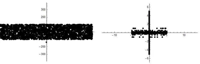
α, β, γ andδare real numbers. Here we focus on contour of the function and the forbidden setFwhere the function has poles inR2.
We are looking for the points (u, v) and parametersβ and δsuch that the rational function has poles and not well defined accordingly. We found such points (u, v) and corresponding parametersβ and δ
Figure 1: Forbidden set of points (u, v) (Left) and associated parameters plot (β, δ) (Right)
A quick reference of members of the forbidden set (FR) is given as
u→0, v→ −761, β→0, δ→ 18
5
,
u→0, v→0, β→ −103
5 , δ→ 176
5
,
u→ −83, v→71, β→2, δ→ 59
5893
,
u→0, v→811, β→0, δ→ −12
5
,
u→ −31, v→82, β→ −5, δ→ −441
2542
,
u→ −229, v→28, β→ 7
2, δ→ − 131 6412
,
u→ −173, v→85, β→ 31
10, δ→ 181 29410
,
u→0, v→ −223, β→0, δ→ 13
10
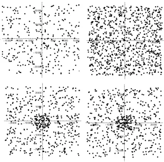
We are also interested to explore the forbidden set for the complex rational function
f(u, v) = α+γu
δuv+u+βv α, β, γ andδare complex numbers.
Figure 2: Forbidden set of pointu(Top left),v(Top Right) and associated parameters plotβ(Bottom Left) andδ (Bottom Right)
A quick reference of members of the forbidden set (FC) is given as
u→1443
10 + 34i, v→ 1923
10 − 2323i
10 , β→ − 2449
10 − 681i
10 , δ→
17100840933528 9993902925521 + 656645917832i 9993902925521 ,
u→ −787
5 − 389i
10 , v→ − 1887
10 − 867i
10 , β→ −213 + 249i, δ→ −
100307231345 111142908363+ 11794709225i 6537818139 ,
u→0, v→ −1947
10 + 23i
2 , β→0, δ→ − 613 10 + 549i 10 , and
u→0, v→0, β→ 93
10− 39i
2 , δ→ − 179
10 + 417i
10
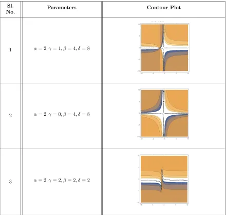
Sl.
No. Parameters Contour Plot
1 α= 2, γ= 1, β= 4, δ= 8
2 α= 2, γ= 0, β= 4, δ= 8
3 α= 2, γ= 2, β= 2, δ= 2
Table 1: Parametersα,γ βandδfor which the fixed points~is attracting, repelling for different initial
values with different delayk.
We are interested to explore the the dynamics of the rational difference equation where (a subset of
R2−FR) the rational function is well defined. We intend to see the dynamics computationally from the
delaykperspective.
3
Local Asymptotic Stability of the Equilibrium
The rational difference equation has only one real fixed point (~(say)) and we shall see the local
asymp-totic stability of the fixed point (~). Here we are looking for parameters α, β, γ and δ with delay k,
Sl. No.
Parameters
α,γ,β,δ &k Remark
1 α=−−7671, γ, δ==−−5962, β=
If the delay k is odd, then the trajectories (for ten different initial values) are attracting to the fixed point 1.01112 which is shownFig. 2.
If the delay k is even then the trajectories are diverging as shown inFig. 2.
2 α= 1721, γ, δ==−−9092, β=
If the delay k is odd, then the trajectories (for ten different initial values) are attracting to a period two cycle which is shownFig. 2.
If the delaykis even then the trajectories are attracting to the fixed point−0.9683 inFig. 2.
Table 2: Parametersα,γ,βandδfor which the fixed points~is attracting, repelling for different initial values with different delayk.
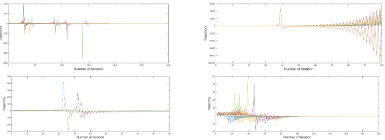
Figure 3: Trajectory plots attracting (Sl No 1) (Above: Left: kis odd, Right: k is even) and repelling (Sl. No. 2) (below: Left: kis odd, Right: kis even) for two different set of parameters with different kinds of delayk.
Sl. No.
Parameters
α,γ,β,δ &k Remark
1 α=−7063, γ, δ== 65−68, β=
If the delay k is odd, then the trajectories (for ten different initial values) are repelling and seems chaotic which is shown
Fig. 3.
If the delay k is even then the trajectories are diverging as shown inFig. 3.
2 α=−−6663, γ, δ==−−9221, β=
If the delay k is odd, then the trajectories (for ten different initial values) are attracting to a period two cycle which is shownFig. 3.
If the delaykis even then the trajectories are chaotic as shown inFig. 3.
Table 3: Parametersα,γ,βandδfor which the fixed points~is attracting, repelling for different initial values with different delayk.
Figure 4: Trajectory plots attracting (Sl No 1) (Above: Left: kis odd, Right: k is even) and repelling (Sl. No. 2) (below: Left: k is odd, Right: kis even) for two different sets of parameters with different kinds of delayk.
In the next two sections, we shall explore the diversity (periodic and chaotic) of dynamics of the rational difference equation Eq.(1) considering the delayk as even and odd separately.
4
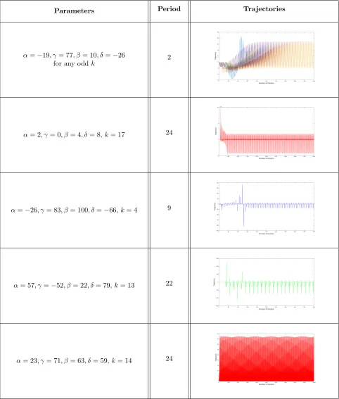
Periodic Solutions
By now we are convinced that there are fixed points of the rational difference equation Eq.(1) which are repelling and hence the trajectories are either chaotic or periodic. We are interested to explore different higher (if exists) order periodic solution of the difference equation Eq.(1).
Parameters Period Trajectories
α=−19, γ= 77, β= 10, δ=−26 for any oddk
2
α= 2, γ = 0, β= 4, δ= 8, k= 17 24
α=−26, γ= 83, β= 100, δ=−66,k= 4 9
α= 57, γ=−52, β= 22, δ= 79,k= 13 22
α= 23, γ= 71, β= 63, δ= 59,k= 14 24
5
Chaotic Solutions
Here we shall explore solutions of the difference equation of type chaotic which are neither converging nor forming cycle. A few examples are taken here for demonstration. Over iterations, none of the trajectories for a specific parameter with different initial values is converging/ not forming cycles.
Consider the parameters α= 9, γ = 16, β = −96, δ = −45 and k = 28, the trajectories for many iterations for ten different sets of initial values are seen to be chaotic. The trajectories for 500, 5000, 10000, 80000 and 100000 iterations are shown inFig. 4.
Figure 5: Trajectory plots for 500, 5000, 10000, 80000 and 100000 iterations where delayk= 28.
Another similar example is considered here. The parametersα=−10,γ= 79,β =−182,δ=−108 and
k= 48, the trajectories for many iterations for ten different set of initial values are seen to be chaotic (ensured by Lyapunav exponent). The trajectories for 500, 5000, 10000, 80000 and 100000 iterations are shown inFig. 5.
Figure 6: Trajectory plots with for 500, 5000, 10000, 80000 and 100000 iterations where delayk= 48.
It is worth noting that the Lyapunav exponent for the two cited examples are found to be positive. So far we have seen the typical dynamics of the rational difference equation Eq.(1). We shall consider the same equation Eq.(1) but with complex variables (parameters and initial values). In biological con-text, the rational function can be thought as a response function of a biological system. The variables
hn is a coupled response of two attributes (viz. (temperature, humidity), etc.). The parameters are
In the following section, we shall explore the dynamics of the equation Eq.(1) in complex plane and see the rationale of the system in coupled scenario.
6
A Glimpse of Coupled Dynamics
Here a set of examples is depicted with variety of dynamical behavior of the rational difference equation Eq.(1) where the variables and parameters are complex (having two attributes). In the followingTable-5, 6 & 7, the attracting, periodic and chaotic dynamics are shown.
Parameters Attracting Nature Trajectories
α= 0.706 + 0.6451i, γ= 0.5523 + 0.2181i, β = 0.7724 + 0.228i, δ=
0.3709 + 0.89909i
for anyk
Attracting to 0.7962−0.0807i
α= 5−94i, γ=−15−67i, β=
−31 + 24i, δ=−84 + 25i,k= 1
Attracting to one of its fixed points 0.800033 + 0.859814i
α= 82−43i, γ= 82−43i, β= 82−43i, δ= 82−43i, for any k
Attracting to a fixed point
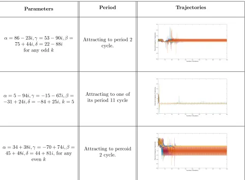
Parameters Period Trajectories
α= 86−23i, γ= 53−90i, β= 75 + 44i, δ= 22−88i
for any oddk
Attracting to period 2 cycle.
α= 5−94i, γ=−15−67i, β=
−31 + 24i, δ=−84 + 25i, k= 5
Attracting to one of its period 11 cycle
α= 34 + 38i, γ=−70 + 74i, β= 45 + 48i, δ = 44 + 81i, for any
evenk
Attracting to percoid 2 cycle.
Table 6: Parameters, Periods and Trajectories with different delayk.
Parameters Nature Trajectories
α= 86−23i, γ= 53−90i, β= 75 + 44i, δ= 22−88i
for any even k
Chaotic, (Lyapunav Exponent of the real
and imaginary trajectories: (1.345,0.563))
α= 5−94i, γ=−15−67i, β=
−31 + 24i, δ=−84 + 25i,
k= 11,13,15,17 and 19
Chaotic, (Lyapunav Exponent of the real
and imaginary trajectories: (0.5643,0.4321))
α= 34 + 38i, γ=−70 + 74i, β= 45 + 48i, δ = 44 + 81i, for any
odd k
Chaotic, (Lyapunav Exponent of the real
and imaginary trajectories: (0.7123,0.98564))
Table 7: Parameters and Chaotic Trajectories with different delayk.
Here we observe the examples as adumbrated in the Table-5, 6 & 7 and make following remarks from delaykperspective. Whenα= 5−94i, γ=−15−67i, β=−31 + 24i, δ =−84 + 25iand if the delayk
is 1, then the trajectories for different initial values are attracting to a fixed point and while the delay
k is 5 then the trajectories are forming periodic cycle of length 11 as shown in the second example of eachTable-5 & 6. And if the delay k= 11,13,15,17 and 19 the trajectories are chaotic which is seen in theTable 7.
In another example when the parameters are set to beα= 34 + 38i, γ=−70 + 74i, β = 45 + 48i, δ= 44 + 81ithen for any evenkthe trajectories are periodic of period 2 and if the delaykis even then the trajectories are chaotic as shown inTable-6 & 7.
7
Special Kind of Complex Dynamics
Parameters Nature Trajectories
α=−13−87i, γ=−13−
87i, β=−13−87i, δ=−13−87i
for anykand then the trajectories are diverging
monotonically
α=−95−17i, γ= 0, β= 0, δ= 0,
for anyk, trajectory is converging to a periodic cycle of
high length.
α= 34 + 38i, γ=−α, β=
−α, δ=−α, for any evenk
Gradually diverging
Table 8: Special Cases of Complex Parameters and Trajectories with different delayk.
8
Special Kind of Real Dynamics
Parameters Nature
α=−170, γ =α, β=−191, δ=β
for anyk= 2 and then the trajectories are gradually diverging monotonically
α=−56, γ=α, β= 70, δ=β
for anyk= 2 and then the trajectories are chaotic with self similarity
(fractal-like).
α= 95, γ =α, β=−40, δ=β
for anyk= 43 and then the trajectory is periodic with high periodicity).
α= 53, γ= 1
α, β= 1, δ= 1 α
for anyk= 15 and then the trajectories are quasi-periodic with
very high quasi-periodicity).
Table 9: Special Cases of Real Parameters and Trajectories with different delayk.
9
Summary and Future Endeavours
of biological systems, the study of rational difference equations is still in its infancy. Although in last two decades, the theoretical understanding of second and third order rational difference equations are sufficiently enriched.
In our future endeavours, we wish to see the dynamics of the most generalized rational difference equation
hn+1 =
α+γhn−k βhn+δhnhn−l+hn−l
, n= 0,1,2, . . .
wherek andlare two different delay terms and it indeed demands similar computational analysis.
Acknowledgement
The authors tender thank to thePingla Thana Mahavidyalaya, Maligram, Paschim Midnapur, 721140, Indiafor facilitating scopes in conducting the present research work successfully.
References
[1] D. C. Zhang and B. Shi, (2003) Oscillation and global asymptotic stability in a discrete epidemic model, J. Math. Anal. Appl. 278 194202.
[2] D. Benest and C. Froeschle, (1998)Analysis and Modeling of Discrete Dynamical Systems (Cordon and Breach Science Publishers, The Netherlands.
[3] Saber N Elaydi, Henrique Oliveira, Jos Manuel Ferreira and Joo F Alves, (2007) Discrete Dyan-mics and Difference Equations, Proceedings of the Twelfth International Conference on Difference Equations and Applications, World Scientific Press.
[4] M.R.S. Kulenovi´c and G. Ladas, (2001)Dynamics of Second Order Rational Difference Equations; With Open Problems and Conjectures, Chapman & Hall/CRC Press.
[5] Y. Saito, W. Ma and T. Hara, (2001) A necessary and sufficient condition for permanence of a LotkaVolterra discrete system with delays, J. Math. Anal. Appl. 256, 162174.
[6] J. R. Beddington, C. A. Free and J. H. Lawton, (1975)Dynamic complexity in predatorprey models framed in difference equations, Nature 255, 5860.
[7] J. Chen and D. Blackmore, (2002) On the exponentially self-regulating population model, Chaos, Solitons Fractals 14, 14331450.
[8] L. Edelstein-Keshet, (1988) Mathematical Models in Biology, Birkhauser Mathematical Series
Birkhauser, New York.
[9] J. D. Murray, (2007) Mathematical Biology: I. An Introduction, Interdisciplinary Applied Mathe-matics Springer, Oxford.
[10] Yanhui Zhai, Xiaona Ma, Ying Xiong (2014) Hopf Bifurcation Analysis for the Pest-Predator Models Under Insecticide Use with Time Delay, International Journal of Mathematics Trends and Technology 9(2) 115-121.