Performance evaluation on optimisation of 200 dimensional numerical tests - results and issues

PERFORMANCE EVALUATION ON OPTIMISATION OF 200 DIMENSIONAL

NUMERICAL TESTS – RESULTS AND ISSUES

Kalin PENEV

Abstract: Many tasks in science and technology require optimisation. Resolving such tasks could bring great benefits to community. Multidimensional problems where optimisation parameters are hundreds and more face unusual computational limitations. Algorithms, which perform well on low number of dimensions, when are applied to high dimensional space suffers insuperable difficulties. This article presents an investigation on 200 dimensional scalable, heterogeneous, real-value, numerical tests. For some of these tests optimal values are dependent on dimensions’ number and virtually unknown for variety of dimensions. Dependence on initialisation for successful identification of optimal values is analysed by comparison between experiments with start from random initial locations and start from one location. The aim is to: (1) assess dependence on initialisation in optimisation of 200 dimensional tests; (2) evaluate tests complexity and required for their resolving periods of time; (3) analyse adaptation to tasks with unknown solutions; (4) identify specific peculiarities which could support the performance on high dimensions (5) identify computational limitations which numerical methods could face on high dimensions. Presented and analysed experimental results can be used for further comparison and evaluation of real value methods.

Key Words: Free Search, 200 dimensional optimisation, black box optimisation

1. INTRODUCTION

A number of publications present evaluation and improvement of existing and design of new methods for resolving multidimensional tasks [5, 6, 10, 11, 15, 16, 20, 21]. However many questions in multidimensional optimisation require satisfactory answers and need additional research.

This article presents an investigation on optimisation of 200 dimensional versions of scalable, heterogeneous, real-value numerical tests. It continues the efforts on multidimensional optimisation published earlier [14]. The number of potential solution for 200 dimensions is large. This makes these tasks difficult for identification and clarification of the optimal solutions with acceptable level of precision.

Earlier publications suggest that available optimisation methods could perform well on variety of tests with low number of dimensions. At the same time when applied to multidimensional tasks with hundreds of parameters these methods face difficulties such as: - need for large number of objective function evaluations (FE); - need for large computational resources; - need for unfeasible large period of time for calculations; - inability to identify optimal solution; - inability to clarify optimal solution with appropriate level of precision [14].

An essential issue, on which this article focuses, is how search processes depend on initialisation. A widely used manner for assessment of some search methods requires: “Uniform random initialization within the search space.” [9] In order to assess whether initialisation could reflect on methods performance presented study compares start from stochastically generated initial solutions with start from one location, where all initial solutions are identical. Start from one initial location allows to assess both abilities for divergence and for convergence and capability to harmonise them.

2. FREE SEARCH

Due to a specific performance identified in earlier investigation [14], optimisation method selected for this study is Free Search (FS) only. This section refines the description of the method published in the literature [12, 13, 14].

Free Search is organised in individual explorations within surrounding neighbour space. On initial stage FS requires definition of the search space boundaries, individuals number, limits for number of explorations, number of steps per exploration, and minimal and maximal values for the neighbour space frame. The maximal neighbour space guarantees coverage of the whole search space by one individual. The minimal neighbour space guarantees desired granularity of the coverage by one individual. An appropriate definition of these values supports good performance across variety of spaces without additional external adjustment. A prior determination of the neighbour space and adjustment of the algorithm for a particular problem based on preceding knowledge can lead to slightly better performance on that problem but aggravates the performance on other problems which concurs with the existing general assessment of the performance of optimisation algorithms [19].

parameters. FS generates a new solution as deviation of a current one: x = x0 + ∆x. Where x is a new solution,

x0 is a current solution and ∆x is modification strategy. x, x0 and ∆x are vectors of real numbers.

Exploration generates coordinates of a new location xtji as:

xtji = x0ji - ∆xtji + 2*∆xtji* randomtji (0,1).

Modification strategy used in the algorithm is:

∆xtji = Rji * ( Xmaxi – Xmini ) * randomtji(0,1).

Where: i indicates dimensions; i = 1,..,n for multi-dimensional step; t is the current step of the individual with the exploration t = 1,..,T; T is the step limit per individual exploration (walk); Xmini and Xmaxi are search

space boundaries. Rji indicates the size of the neighbourhood space for individual j within the dimension i.

randomtji(0,1) generates random values between 0 and 1. ∆xtji indicates the actual size of the neighbourhood

space for a particular problem for step t of individual j within dimension i.

During the exploration an individual, which can do large steps that exceeds search space boundaries, can perform global search whereas another individual, which can do small steps can perform precise search around one location.

The modification strategy is independent from the current or the best achievements. The individual exploration is followed by an, also, individual assessment of the explored locations.

The best location for each individual is marked according to the quality known from current and previous explorations. This indicates the relative quality of the locations and could be classified as cognition about the search space. Marked locations normalise the explored problem to an idealised qualitative (or cognitive) space, in which the algorithm operates. The normalisation of any particular search space to one idealised space supports successful performance across variety of problems without additional external adjustments. The process continues with selection of a start location for a new exploration. Selection is based on stochastically generated individual sense and locations quality. After the explorations follows termination. Acceptable criteria for termination are reaching the optimisation criterion, expiration of the generations’ limit or complex criterion. [12, 13, 14]

3. NUMERICAL TESTS

For evaluation of abilities for adaptation to variety of problems without retuning, several scalable heterogeneous tests are selected: - global optimisation tests with attractive local suboptimal solutions - Michalewicz and Norwegian; - tests with many suboptimal peaks on one global hill - Griewank, Rastrigin and Schwefel; - flat test with maximum located on the top of flat hill, difficult to be differentiated among very similar neighbour locations - Rosenbrock; - test with no local correlation between the solutions - Step; - hard constrained global optimisation test - Bump. In addition the optimal solutions for Michalewicz, Norwegian and Bump tests are dependent on dimensions number and virtually unknown. All selected tests are scaled to 200 dimensions.

3.1. Michalewicz test

Michalewicz test is referred in the literature [6] as global optimisation problem. In this study it is transformed for maximisation.

m n

i

i i

i x ix

x

f 2

1

2 )) / )(sin( sin( )

(

∑

π

=

=

where search space is defined as 0 ≤ xi ≤ π, i = 1, . . . , n. The maximum is dependent on dimensions

number and for n = 200 is unknown.

3.2. Norwegian test

Norwegian test is global test problem [2].

( )

_∏

= 

 

 

    

 +

= n

i

i i

i

x x x

f

1

3

100 99 ) cos(π

where search space borders are defined by –1.1< xi <1.1, i = 1, . . . , n. The maximum is dependent on

3.3. Rosenbrock test

Rosenbrock test landscape is smooth flat hill with one optimal solution [17]. The function is:

∑

− = +

−

+

−

−

=

1 1 2 2 2

1

)

(

1

)

]

(

*

100

[

)

(

n i i i i

i

x

x

x

x

f

Where xi∈ [-2, 2] and i = 1,..,n-1. It has one maximum fmax = 0, for xi = 1, i = 1,..,n.

3.4. Griewank test

The test [4], is given by the following analytical expression:

( )

2

1 1 1 1 cos 4000 n n i i i i i x

f x x

i = =   = + − _{ }  

∑ ∏

where xi∈ [-600.0, 600.0]. The maximum is fmax = 0, for xi = 0, i = 1,..,n.

3.5. Rastrigin test

This test function is known from the literature [18].

))

2

cos(

(

)

(

1 2

∑

=

−

+

=

n i i

i

A

x

x

nA

x

f

π

where A=10 and –5.12< xi <5.12. The maximum is fmax = 0, for xi = 0, i = 1,..,n.

3.6. Step test

Step test [3] introduces plateaus to the topology, which excludes local correlation. Maximal are all locations for xi∈ [2.0, 2.5). The maximum is dependent on dimensions number. The test function is:

 

∑

=

=

n i i i

x

x

f

1

)

(

where xi∈ [-2.5, 2.5]. For n = 200 the maximum is fmax = 400, for xi∈ [2.0, 2.5), i = 1,..,n.

3.7. Schwefel test

Schwefel test is referred in the literature [1]. In this study is transformed for maximisation:

( )

i

n

i i

i n x x

x

f( ) 418.9829* sin 1

∑

=

− =

where n is number of dimensions and - 500 ≤ xi ≤ 500, i=1,…,n. The maximum is 0.

3.8. Bump test

This is hard constrained global optimisation problem [8] transformed in this study for maximisation.

∑

∏

∑

= = = − = n i i n i i i n i

i x x ix

x f 1 2 1 2 1

4_{( ) 2 cos ( )/}

cos )

(

Subject to: 0.75

1 >

∏

= n i i

x

and

15 /2

1 n x n i i<

∑

=

for: 0 < xi < 10, and i =1,…,n, start from xi = 5, i =1, . . . ,n, where xi are the variables (expressed in radians)

4. EXPERIMENTAL METHODOLOGY

Experiments are organised in two sections with different initialisations - start from one location and start from random locations. Selected test are implemented for 200 dimensions. Individuals number for all experiments is n = 10.

For the first section initialisation is start from one identical for all experiments location, defined as:

xi0 = Xmin + 0.1*(Xmax - Xmin)

where Xmax and Xmin are search space borders, i = 1,..,n is individual’s number.

In this section two series of 320 experiments are conducted. First series are limited to 2.106 _{and second to}

2.108 _{function evaluations (FE).}

For second section initialisation is start from stochastically generated initial locations different for each experiment. Start locations for these experiments are defined as:

xi0 = Xmin + randomi (Xmax - Xmin)

where Xmax and Xmin are search space borders and randomi (Xmax - Xmin) generates random value between

Xmax and Xmin, i = 1,..,n. All variables are 200 dimensional vectors.

In this section two series of 320 experiments, are completed as well. For first series limit is 2.106 _{and for}

second 2.108 _FE.

5. EXPERIMENTAL RESULTS

Achieved from each series of 320 experiments results are analysed for maximal and mean values, standard deviation and number of results which are with precision 0.01 from the maximal value.

Table 1. Maximal results from 320 experiments

Table 2. Statistics for start from one location from 320 experiments

Function evaluations One location Random locations Schwefel 2.106 _{-0.0538755 -0.0557508}

2.108 _{-0.00187438 -0.00177903}

Michalewicz 2.106 _{199.596 199.595}

2.108 _{199.613 199.612}

Norwegian 2.106 _{0.919569 0.919469}

2.108 _{1.00007 1.00007}

Rosenbrock 2.106 _{-175.4057741 -142.1966488}

2.108 _{-0.002175406 -0.00000246422}

Griewank 2.106 _{-0.000000491282 -0.000000548503}

2.108 _{-0.0000000189166 -0.0000000217225}

Rastrigin 2.106 _{-0.000000741589 -0.000000872608}

2.108 _{-0.0000000254734 -0.000000022934}

Step 2.106 _{400 400}

2.108 _{400 400}

Function evaluations

Mean results Standard deviation Schwefel 2.106 _{-0.09531892 0.01728344}

2.108 _{-0.002993843 0.000609849}

Michalewicz 2.106 _{199.5813469 0.006815538}

2.108 _{199.6084344 0.001768317}

Norwegian 2.106 _{0.857017675 0.024420224}

2.108 _{0.980172659 0.01027313}

Rosenbrock 2.106 _{-228.4110106 48.41659519}

2.108 _{-142.7193144 35.55148446}

Griewank 2.106 _{-0.007593595 0.013003385}

2.108 _{-0.00516372 0.008218812}

Rastrigin 2.106 _{-0.0000045002 0.00000225244}

2.108 _{-0.000000123029 0.0000000701082}

Step 2.106 _{400 0}

Table 3. Statistics for start from random locations from 320 experiments

Table 4. Number and percentage of the results with precision above 0.01

Table 5. Period of time for 2.108 _{objective function evaluations}

All experimental results are achieved by Free Search [12] with its standard parameters. Time periods in Table 5 are measured on processor Intel i7 3960x overclocked to 4747 MHz and memory G.Skill TridentX at 1885 MHz, motherboard ASUS Rampage VI and solid state disk - SanDisk Extreme SSD SATA III.

In order to evaluate more rigorously level of potentially achievable precision additionally Bump test only is explored for 200 dimensions with start from one location.

For start location is used f200-start= 0.85116941245212996.

Best achieved solutions from 320 experiments limited to 2.106 _{FE and to 2.10}8 _{FE are:}

f200-2M FE = 0.851169412452639 and f200-200M FE = 0.85116941245573432 accordingly.

As far as optimal value for this test is unknown statistical analysis is skipped. This result illustrates the power of heuristics search, where accidental events could help to discover (eureka) or identify desired solution. It should be noted that: (1) these results are achieved on probabilistic principle; (2) the search space is continuous and the results can be clarified to an arbitrary precision. Free Search itself has no limitations to clarify this result with arbitrary precision. However modern computer systems limit this clarification due to the floating point format for representation of real numbers.[7]

Function evaluations Mean results Standard deviation Schwefel 2.106 _{-0.094394835 0.018476771}

2.108 _{-0.003024044 0.000615262}

Michalewicz 2.106 _{199.5814969 0.006683935}

2.108 _{199.6084094 0.001784807}

Norwegian 2.106 _{0.857816916 0.025250762}

2.108 _{0.9795565 0.009963986}

Rosenbrock 2.106 _{-280.4516787 53.28420889}

2.108 _{-73.81542886 55.5996416}

Griewank 2.106 _{-0.007250139 0.011809403}

2.108 _{-0.004964609 0.007490583}

Rastrigin 2.106 _{-0.00000407817 0.00000230627}

2.108 _{-0.000000122502 0.000000071005}

Step 2.106 _{400 0}

2.108 _{400 0}

Function evaluations One location Random locations Schwefel

>-0.00

2.106 _{0 00.00% 0 00.00%}

2.108 _{320 100.00% 320 100.00%}

Michalewicz >199.59

2.106 _{47 14.68% 44 13.75%}

2.108 _{320 100.00% 320 100.00%}

Norwegian >0.99

2.106 _{0 00.00% 0 00.00%}

2.108 _{32 10.00% 26 8,12%}

Rosenbrock >-0.00

2.106 _{0 00.00% 0 00.00%}

2.108 _{1 00.31% 6 01.87%}

Griewank >-0.00

2.106 _{237 74.06% 239 74.68%}

2.108 _{247 77.18% 252 78,75%}

Rastrigin >-0.00

2.106 _{320 100.00% 320 100.00%}

2.108 _{320 100.00% 320 100.00%}

Step >399

2.106 _{320 100.00% 320 100.00%}

2.108 _{320 100.00% 320 100.00%}

6. DISCUSSION

Analysis of experimental results suggests that 200 dimensional Step and Rastrigin tests can be resolved for any initialisation with up to fifth digits precision within 2.106 _{function evaluations (FE) which on used}

computer takes around one minute.

Michalewicz and Griewank can be resolved with precision 0.01 within 2.106 _{FE with probability around}

14% and 74% respectively. Michalewicz test can be resolved with precision 0.01 within 2.108 _{FE for any}

initialisation. Griewank can be resolved with precision 0.01 within 2.108 _{FE with probability around 77%.}

Schwefel, Norwegian and Rosenbrock tests cannot be resolved for 2.106 _{FE with precision 0.01. Schwefel}

test can be resolved for 2.108 _{FE with precision 0.01 for any initialisation.}

Norwegian test can be resolved with precision 0.01 within 2.108 _{FE with probability 8% - 10%. Rosenbrock}

test can be resolved with precision 0.01 within 2.108 _{FE with probability around 1%. Resolving Norwegian and}

Rosenbrock tests with high probability needs higher number of function evaluations.

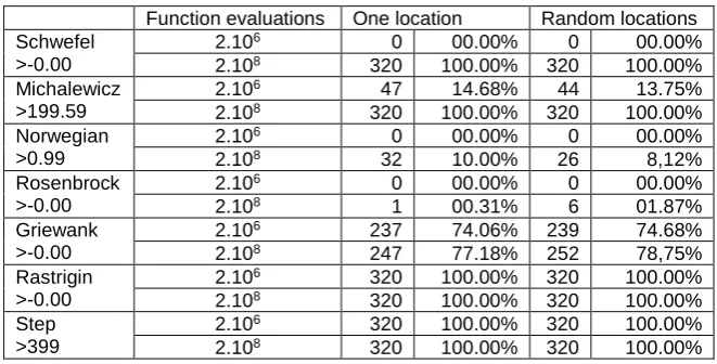
6.1. Dependence on initialisation

A comparison of the presented on Figure 1 numbers of results with precision 0.01 achieved for start from one location and for start from random locations limited to 2.106 _{and 2.10}8 _{function evaluations (indicated on}

the figure as 2M FE and 200M FE respectively) suggests that initialisation does not reflect essentially on the success of the search process for 200 dimensional tasks. This slightly differs from the evaluation of dependence on initialisation for optimisation of 2 dimensional tests published earlier [13].

Fig. 1. Results for one location and random locations initialisations

6.2. Test complexity and period of time

Other core issue for multidimensional search is the period of time required for successful search process completion. The average from 320 experiments, periods of time in minutes, required for completion of one experiment limited to 2.108 _{FE on explored tests for boot - start for one location and start from random locations}

are measured for completeness and presented in Table 5. The results confirm that no reason to expect difference between equal number objective functions evaluation.

However, although the number of function evaluations for all test is equal - 2.108_{, the periods of time vary}

significantly. For used optimisation method this period consists of several components amongst which are: 1) Time for generation of new feasible solutions;

2) Comparison and assessment of generated solutions; 3) Building and updating knowledge about the search space; 4) Selection of positions for next exploration.

Bump test is the most time consuming. Due to the hard constraint, generation of feasible solutions takes additional tame. Michalewicz test is second time consuming, due to the slow calculation of the objective function. Rosenbrock and Step tests are less time consumable. The rest of the tests take medium time for completion. Low period of time for Rosenbrock and Norwegian tests allows these tests to be explored for more FE. Additional experiments shows that Rosenbrock test can be resolved with precision 0.01 with probability 75% within 2.109 _{FE. Average period of time is 64 min. Norwegian tests can be resolved with precision 0.01}

6.3. Unknown optimal solutions

Optimal solutions for Michalewicz Norwegian and Bump tests are dependent on dimensions number and for 200 dimensions are virtually unknown. Best achieved results for these tests are for Michalewicz - 199.613, for Norwegian – 1.00009, and for Bump - 0. 85116941245573432. Clarification of these results could be a subject of further research.

6.4. Search performance in high dimensional space

High dimensional tasks need sufficient number of objective function evaluations. This study demonstrates that for different tasks this number can vary. Appropriate limit within which tasks could be resolved with high probability seems to be between 2.106 _{and 2.10}9_{. Proof or disprove of this could be a subject of further}

research.

Usually for exploration of high dimensional tasks are employed large computational resources. This study demonstrates that with appropriate software methods computational resources could be utilised more effectively.

Analysis of earlier publications shows little evidence that exciting methods could identify optimal solution in particular on global optimisation or on tests where optimal value is unknown. [5][6][10][11][14][15][16][20][21] Presented results confirms that abilities to start and operate from one location and to harmonise divergence and convergence support successful search within multidimensional space.

In real value optimisation the number locations which could be a potential solution depends on required precision. For example for Michalewicz test for search space from 0 to π for 200 dimensions number of locations with precision 0.1 is π*10200 _{and the number of locations with precision 0.01 is} π_*(102₎200₌ π_*10400_.

Presented results demonstrate the number of locations which should be evaluated so that used method could clarify the solution with required level of precision. If higher precision is required then the number of function evaluation should be increased.

6.5. Computational limitations on high dimensional search

One of the cognitive assets, which has significant contribution to the current state of the art in Evolutionary Computation and Computational Intelligence is so called ‘No Free Lunch Theorems in Optimization’ [19]. It proves that “for any algorithm, any elevated performance over one class of problems is offset by performance over another class” [19 p.67]. Prove and scope of these theorems are based on several assumptions amongst which is: “Under the oracle-based model of computation any measure of the performance of an algorithm after m iterations is a function of the sample dmy. … Note that measures of performance based on factors other than

dmy (e.g., wall clock time) are outside the scope of our results.” [19 p.69].

This study identified that computational limitations which numerical methods could face on high dimensional tasks are two – time (e.g., wall clock time plays significant role for optimisation and consequently should be considered for assessment of algorithms performance) and format for representation of real numbers. Time, which some methods require for resolving multidimensional tasks, seems infeasible [14]. In addition the results in Table 5 confirm that the time which different tasks require also vary considerably [14]. With respect to the Chronos this study uses two approaches to overcome time limits – software and hardware.

Regarding the software aspect, used method is fast and capable to produce successful results with high probability within acceptable period of time [14].

Regarding the hardware aspect, used computer system is intentionally designed to be fast with processor Intel i7 3960x overclocked to 4747 MHz and memory G.Skill TridentX at 1885 MHz, which compared to conventional computers decreases the time for calculations more than 30%. Regarding to the representation of real numbers this study requires 64 bit format for floating point representation of real numbers.

Bump test has condition start from xi = 5 and constraint condition

75 . 0

1

>

∏

= n

i i

x

where i = 1,..n is dimensions number.

For n = 200 for start from xi = 5 constraint is 5200 which tends to 6.223*10139. Such large constraint cannot

be represented with standard 32 bit format for floating point representation [7]. For n > 440 start from xi = 5

generates extra-large constraint and 64 bit standard format for floating point representation [7] becomes unusable. In this case either 128 format should be used or start condition could be modified to xi = 1. Other

solution could be development of new standard and more flexible and effective format for representation of real numbers.

7. CONCLUSION

completion of the search process. Identified is required number of objective function evaluations for which selected tests could be resolved with certain probability within acceptable period of time.

Further investigation could focus on evaluation and measure of time and computational resources sufficient for completion of other multidimensional tasks or for higher number of dimensions until reaching the capabilities limits of modern computational systems. Algorithms analysis and improvement could be also subject of future research.

ACKNOWLEDGMENTS

I would like to thank to my students Adel Al Hamadan, Asim Al Nashwan, Dimitrios Kalfas, Georgius Haritonidis, and Michael Borg for the design, implementation and overclocking of desktop PC used for completion of the experiments presented in this article.

REFERENCES

1. Bäck T. and Schwefel H.P., (1993), “An overview of evolutionary algorithms for parameter optimization”, Evolutionary Computation, vol. 1, no. 1, pp 1-23

2. Brekke E. F., (2004), Complex Behaviour in Dynamical Systems, The Norwegian University of Science and Technology, http://www.academia.edu/545835/COMPLEX_BEHAVIOR_IN_DYNAMICAL_SYSTEMS pp 37-38, last visited 10.11.2014.

3. De Jung K. A., (1975), An Analysis of the Behaviour of a Class of Genetic Adaptive Systems, PhD Thesis, University of Michigan.

4. Griewank, A. O., (1981), "Generalized Decent for Global Optimization." Journal of Optimization Theory and Applications, 34, pp. 11-39,

5. Hendtlass, T., (2009), Particle Swarm Optimization and High Dimensional Problem Spaces, IEEE Congress on Evolutionary Computation (CEC 2009), pp 1988 - 1994.

6. Hedar, A.-R., (2014), Test Functions for Unconstrained Global Optimization http://www-optima.amp.i.kyoto-u.ac.jp/member/student/hedar/Hedar_files/TestGO_files/Page2376.htm last visited 10.11.2014

7. IEEE 754, (2008), IEEE 754: Standard for Binary Floating-Point Arithmetic, http://ieeexplore.ieee.org/stamp/stamp.jsp?tp=&arnumber=4610935 last visited 10.11.2014

8. Keane, A.J. (1996) A brief comparison of some evolutionary optimization methods. In, Rayward-Smith, V.J., Osman, I.H., Reeves, C.R. and Smith, G.D. (eds.) Modern Heuristic Search Methods. Chichester, UK, John Wiley, pp. 255-272.

9. Liang, J. J., Qu, B-Y., Suganthan, P. N., (2014), Problem Definitions and Evaluation Criteria for the CEC 2014 Special Session and Competition on Single Objective Real-Parameter Numerical Optimization", Technical Report 201311, December 2013. http://www.ntu.edu.sg/home/EPNSugan/index_files/CEC2014/CEC2014.htm last visit-ed 16.09.2014

10. MacNish, C., Xin Yao, (2008), Direction matters in high-dimensional optimisation. IEEE Congress on Evolutionary Computation, pp 2372-2379

11. Noman, N., Hitoshi Iba, (2005), Enhancing differential evolution performance with local search for high dimensional function optimization, Proceedings of the 2005 conference on Genetic and evolutionary computation, pp 967-974

12. Penev K., and Littlefair G., (2005), Free Search – A Comparative Analysis, Information Sciences Journal, Elsevier, Volume 172, Issues 1-2, pp 173-193.

13. Penev, K., (2009). Adaptive intelligence - Essential aspects. Journal Information Technologies and Control, ISSN 1312-2622, VII (4), pp. 8-17

14. Penev, K., (2013) Free Search – Comparative Analysis 100. Int. J. Metaheuristics, Vol. 3, No. 1, pp 22-33 15. Pu Liu, Francis C. C. Lau, Michael J. Lewis, Cho-Li Wang, 2002, A New Asynchronous Parallel Evolutionary Algorithm for Function Optimization, Proceedings of the 7th International Conference on Parallel Problem Solving from Nature, Springer-Verlag London, UK , pp 401-410

16. Pu Liu and Michael J. Lewis, 2002, Communication Aspects of an Asynchronous Par-allel Evolutionary Algorithm, Proceedings of the Third International Conference on Communications in Computing , Las Vegas, NV, June 24 - 27, 2002, pp. 190-195.

17. Rosenbrock H.H., (1960), An automate method for finding the greatest or least value of a function. Comput. J. 3 (1960), pp.175-184.

18. Torn A., and Zilinskas A.,(1989), Global Optimization, Lecture Notes in Computer Science 350, Berlin, Springer. 19. Wolpert, D.H., and Macready, W. G., (1997), No Free Lunch Theorems for Optimiza-tion, IEEE Transactions on Evolutionary Computation, Vol. 1, No. 1, April 1997, pp 67 - 82

20. Zhenyu Yanga, Ke Tanga, Xin Yaoa, (2008), Large scale evolutionary optimization using cooperative coevolution, Information Sciences, Volume 178, Issue 15, 1 August 2008, pp 2985–2999

21. Zhenyu Yang, Ke Tang, Xin Yao, (2007), Differential evolution for high-dimensional function optimization, IEEE Congress on Evolutionary Computation, 25-28 Sept. 2007, pp 3523 – 3530

CORRESPONDENCE