R E S E A R C H
Open Access
The boundary value problem of a
three-dimensional generalized thermoelastic
half-space subjected to moving rectangular
heat source
Hamdy M. Youssef
1,2*and Eman A.N. Al-Lehaibi
3*Correspondence:
1Mathematics Department, Faculty
of Education, Alexandria University, Alexandria, Egypt
2Mechanics Department, Faculty of
Engineering, Umm Al-Qura University, Makkah, Saudi Arabia Full list of author information is available at the end of the article
Abstract
This paper deals with a new mathematical model of three-dimensional generalized thermoelasticity which has been improved using Lord–Shulman theory. The governing equations on non-dimensional forms have been applied to a
three-dimensional half-space subjected to a rectangular moving heat source and traction-free surface by using the Laplace and double Fourier transform techniques. The inverses of the double Fourier and Laplace transforms have been calculated numerically by applying the complex formula of inversion of the transform by of the Fourier expansion method. The numerical results of the temperature increment, strain, stress, and displacement distributions have been represented in graphs for various values of the heat source speed parameter to show its effect on the thermo-mechanical waves. The heat source speed parameter leads to significant effects on both the thermal and mechanical waves.
Keywords: Three-dimensional modeling; Thermoelasticity; Laplace transforms; Double Fourier transforms; Moving heat source
1 Nomenclature
λ,μ Lame’s parameters
ρ Density
CE Specific heat of the material with constant strain t Time
T Absolute temperature
T0 Reference temperature
θ = (T–T0)Temperature increment
αT Linear thermal expansion coefficient γ =αT(3λ+ 2μ)
σij Stress tensor eij Strain tensor
ui Displacement components K Thermal conductivity
τo Relaxation time
co =
λ+2μ ρ
η =ρKCE
ε = γ2T0 ρCE(λ+2μ) β = (λ+2μμ)1/2
2 Introduction
The difficulty in applications and in solving problems by using the mode of the Fourier transform is how the boundary conditions will be transformed. The important functions have been adapted by order and integrals of the eigenfunctions, depending on a definite system of coordinates (Morse, Feshbach [12]). To obtain the stresses and displacements, dissimilar derivatives of weight must be suited. Satisfying the limit conditions is a some-what perplex work due to the appearance of elasticity coefficients in distinct and high powers in the denominators of the equations (Musii [13]). Podil’chuk and Kirichenko used the Fourier method (Podnil’Chuk, Kirichenko [16]) to construct a new approach for cal-culating the exact solutions to three-dimensional thermoelasticity problems in different coordinate systems.
A lot of numerical and computational methods can be found in viscoelasticity and ther-moelasticity research (Danyluk et al. [2]; Oza et al. [14]; Vinogradov, Milton [21]). Laplace transform method is one of the well-known methods for thermoelasticity and viscoelas-ticity. De Chant used the numerical inversion rule and its limitations in the asymptotic and discontinuities methods (De Chant [3]). Temel got the solutions by applying the nu-merical method of Durbin using the Laplace transform inversions in the real space (Temel et al. [19]). Because of the intricacy of the determining relations, it is very difficult to gain the exact solutions of thermoelasticity, and the numerical approach has been preferred lately with the advances in the information processing system software incorporating the boundary and finite element methods (Mesquita, Coda [11]).
et al. [8]). The global stability of rarefaction waves for the compressible Navier–Stokes equations has been investigated in (Duan et al. [4]).
In this work, a new mathematical model of three-dimensional generalized thermoelas-ticity will be constructed by using Lord–Shulman model. The governing equations on non-dimensional forms will be applied to a three-dimensional half-space subjected to a rectangular moving heat source and traction-free surface by using the Laplace and double Fourier transform techniques. The numerical results of the temperature increment, strain, stress, and displacement distributions will be represented in figures for various values of the heat source speed parameter to show its effect on the thermomechanical waves.
3 The basic equations
The system of partial differential equations of a homogeneous and isotropic thermoelastic medium based on the generalized thermoelasticity with one relaxation time and without any external body forces in undefined coordinates{i,j,k= 1, 2, 3}takes the following form (Ezzat, Youssef [5]; Youssef, Al-Lehaibi [25]):
The equations of motion are
μui,jj+ (μ+λ)uj,ij– (3λ+ 2μ)αθ,i=ρu¨i, (1)
whereθ= (T–T0) is the increment of the temperatureTsuch that|T–T0|/T01.
The heat equation is
Kθ,ii=
∂ ∂t+τ0
∂2 ∂t2
[ρCEθ+γT0e] –
1 +τ0
∂ ∂t
Q. (2)
The constitutive relations are
σij= 2μeij+λekkδij–γ θ δij. (3)
The displacement relation with the strain takes the form
eij=
1
2(ui,j+uj,i). (4)
4 Problem formulation
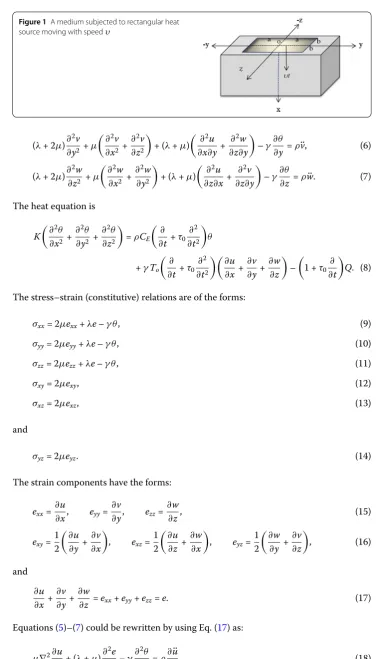
Assume an isotropic, homogeneous and thermoelastic body in three dimensions occupies the regionΨ={x,y,z: 0≤x<∞, –∞<y<∞, –∞<z<∞}where the body is quiescent initially and is loaded thermally by a moving heat source with constant speedυ, which starts from the bounding plane of the surfacex= 0 and moves along thex-axis when these surfaces are traction-free as in Fig.1. The basic equations will be constructed in the context of Lord and Shulman model (L–S). The Cartesian coordinates (x,y,z) will be used, and the displacement components ofui= (u,v,w) are set as follows (Ezzat, Youssef [5]; Youssef,
Al-Lehaibi [25]):
The equations of motion are
(λ+ 2μ)∂
2u
∂x2 +μ
∂2u
∂y2 +
∂2u
∂z2
+ (λ+μ)
∂2v
∂x∂y+ ∂2w
∂x∂z
–γ∂θ
Figure 1A medium subjected to rectangular heat source moving with speedυ
(λ+ 2μ)∂
2v
∂y2+μ
∂2v
∂x2+
∂2v
∂z2
+ (λ+μ)
∂2u
∂x∂y+ ∂2w
∂z∂y
–γ∂θ
∂y=ρv¨, (6)
(λ+ 2μ)∂
2w
∂z2 +μ
∂2w ∂x2 +
∂2w ∂y2
+ (λ+μ)
∂2u ∂z∂x+
∂2v ∂z∂y
–γ∂θ
∂z =ρw¨. (7)
The heat equation is
K
∂2θ
∂x2 +
∂2θ
∂y2 +
∂2θ
∂z2
=ρCE
∂ ∂t+τ0
∂2
∂t2
θ
+γTo
∂ ∂t+τ0
∂2 ∂t2
∂u ∂x +
∂v ∂y+
∂w ∂z
–
1 +τ0
∂ ∂t
Q. (8)
The stress–strain (constitutive) relations are of the forms:
σxx= 2μexx+λe–γ θ, (9)
σyy= 2μeyy+λe–γ θ, (10)
σzz= 2μezz+λe–γ θ, (11)
σxy= 2μexy, (12)
σxz= 2μexz, (13)
and
σyz= 2μeyz. (14)
The strain components have the forms:
exx= ∂u
∂x, eyy= ∂v
∂y, ezz= ∂w
∂z, (15)
exy=
1 2
∂u ∂y+
∂v ∂x
, exz=
1 2
∂u ∂z +
∂w ∂x
, eyz=
1 2
∂w ∂y +
∂v ∂z , (16) and ∂u ∂x +
∂v ∂y+
∂w
∂z =exx+eyy+ezz=e. (17)
Equations (5)–(7) could be rewritten by using Eq. (17) as:
μ∇2∂u
∂x+ (λ+μ) ∂2e ∂x2 –γ
∂2θ ∂x2 =ρ
∂u¨
μ∇2∂v
∂y+ (λ+μ) ∂2e
∂y2 –γ
∂2θ
∂y2 =ρ
∂v¨
∂y, (19)
μ∇2∂w
∂z + (λ+μ) ∂2e ∂z2 –γ
∂2θ ∂z2 =ρ
∂w¨
∂z, (20)
where
∇2= ∂2
∂x2+
∂2 ∂y2 +
∂2 ∂z2.
The heat conduction equation takes the form
K∇2θ=ρCE
∂ ∂t+τ0
∂2
∂t2
θ+γTo
∂ ∂t+τ0
∂2
∂t2
e–
1 +τ0
∂ ∂t
Q. (21)
Now, the following dimensionless variables will be applied (Ezzat, Youssef [5–7]):
x∗,y∗,z∗=cη(x,y,z), t∗,τ0∗=c2η(t,τo), θ∗= γ θ
(λ+ 2μ),
Q∗= Q
Kc2η2T
o
, σij∗= σij
λ+ 2μ, c=
λ+ 2μ
ρ , η= ρCE
K .
Thus, we obtain
β∇2∂u
∂x+ (1 –β) ∂2e ∂x2 –
∂2θ ∂x2 =
∂u¨
∂x, (22)
β∇2∂v
∂y+ (1 –β) ∂2e ∂y2 –
∂2θ ∂y2 =
∂v¨
∂y, (23)
β∇2∂w
∂z + (1 –β) ∂2e
∂z2 –
∂2θ
∂z2 =
∂w¨
∂z, (24)
∇2θ=
∂ ∂t+τ0
∂2 ∂t2
θ+ε1
∂ ∂t+τ0
∂2 ∂t2
e–ε2
1 +τ0
∂ ∂t
Q, (25)
σxx= 2βexx+ (1 – 2β)e–θ, (26)
σyy= 2βeyy+ (1 – 2β)e–θ, (27)
σzz= 2βezz+ (1 – 2β)e–θ, (28)
σxy= 2βexy, (29)
σxz=βexz, (30)
σyz= 2βeyz, (31)
where
β= μ
λ+ 2μ, ε1=
γ2T0
ρCE(λ+ 2μ)
, ε2=
γT0
(λ+ 2μ).
By taking the sum of the Eqs. (22)–(24) and substituting Eq. (17), we get
∇2e–∇2θ=e¨. (32)
We will assume the functionσis the invariant stress, which is given as follows:
σ=σxx+σyy+σyy
3 . (33)
By using Eqs. (26)–(28), we obtain
σ=αe–θ, (34)
where
α=3 – 4β
3 .
5 Applying the Laplace transform on the governing equations
We will be using Laplace transform, which is defined for any functionG(t) as follows:
¯
G(s) =
∞
0
G(t)e–stdt. (35)
Applying the transform to (35), we obtain:
β∇2∂u¯
∂x+ (1 –β) ∂2¯e ∂x2 –
∂2θ¯ ∂x2 =s
2∂u¯
∂x, (36)
β∇2∂v¯
∂y+ (1 –β) ∂2¯e ∂y2 –
∂2θ¯ ∂y2 =s
2∂v
∂y, (37)
β∇2∂w¯
∂z + (1 –β) ∂2e¯ ∂z2 –
∂2θ¯ ∂z2 =s
2∂w¯
∂z, (38)
∇2e¯–∇2θ¯=s2e¯, (39)
∇2θ¯=s+τ 0s2
¯ θ+ε1
s+τ0s2
¯
e–ε2(1 +τ0s)Q¯, (40)
¯
σxx= 2βe¯xx+ (1 – 2β)¯e–θ¯, (41)
¯
σyy= 2βe¯yy+ (1 – 2β)e¯–θ¯, (42)
¯
σzz= 2βe¯zz+ (1 – 2β)e¯–θ¯, (43)
¯
σxy= 2β¯exy, (44)
¯
σxz=βe¯xz, (45)
¯
σyz= 2βe¯yz, (46)
¯
Using the Laplace transform, we applied the following initial conditions:
u(r,t)
t=0
=v(r,t)
t=0
=w(r,t)
t=0
=θ(r,t)
t=0
= 0,
∂u(r,t)
∂t
t=0
=∂v(r,t)
∂t
t=0
=∂w(r,t)
∂t
t=0
=∂θ(r,t)
∂t
t=0
= 0, r=x,y,z.
(48)
We assumed the medium is subjected to a rectangular heat source moving with con-stant speed and concon-stant strength, releasing its energy continuously on a band of concon-stant dimensions 2a×2bcentered on they-axis andz-axis, respectively, while moving with constant speedυalong thex-axis and being zero elsewhere as in Fig.1.
Thus, the rectangular moving heat source is assumed to be of the following dimension-less form [22]:
Q=Qoδ(x–υt)H
a–|y|Hb–|z|, (49)
whereaandbare constants,Qois the heat source strength (constant),δis the Dirac delta
function, andH(t) is the Heaviside function. Applying the Laplace transform, we get
Q=Qo
υ H
a–|y|Hb–|z|e–(υs)x. (50)
Eliminatinge¯in Eqs. (39), (40) and (47), we get
∇2σ¯=α
1θ¯+α2σ¯–γ1H
a–|y|Hb–|z|e–(υs)x (51)
and
∇2θ¯=α
3θ¯+α4σ¯–γ2H
a–|y|Hb–|z|e–(υs)x, (52)
where
α1=
s2α– (s+τ
0s2)(1 –α)(α+ε1)
α , α2=
s2α–ε 1(1 –α)
α ,
α3=
(s+τ0s2)(α+ε1)
α , α4=
ε1(s+τ0s2)
α ,
γ1=ε2(1 +τ0s)(α– 1)
Qo
υ , γ2=ε2(1 +τ0s) Qo
υ .
6 Applying the double Fourier transform
The double Fourier transform for any functionf(x,y,z) is defined as follows:
Ff¯(x,y,z,s)=f˜¯(x,p,q,s) = 1 2π ∞ –∞ ∞ –∞ ¯
f(x,y,z,s)e–i(py+qz)dy dz, (53)
where the inverse of the double Fourier transform takes the form
F–1f˜¯(x,p,q,s)=f¯(x,y,z,s) = 1 2π ∞ –∞ ∞ –∞ ˜¯
Thus, we have
F∇2f¯(x,y,z,s)=
d2
dx2 –q 2–p2
˜¯
f(x,p,q,s). (55)
Applying the transforms to (53) and (55), we get the following ordinary differential equa-tions:
d2σ˜¯
dx2 =α1θ˜¯+β1σ˜¯ –γ3e
–(υs)x (56)
and
d2θ˜¯
dx2 =β2θ˜¯+α4σ˜¯ –γ4e
–(υs)x, (57)
where
β1=p2+q2+α2, β2=p2+q2+α3,
γ3=
2
π
γ1sin(qa)sin(pa)
qp , and γ4=
2
π
γ2sin(qb)sin(pb)
qp .
Eliminatingσ˜¯ from Eqs. (56) and (57), we get
d4
dx4 – (β1+β2)
d2
dx2 + (β1β2–α1α4)
˜¯
θ= –β5e–
s
υx. (58)
Similarly, eliminatingθ˜¯from Eqs. (56) and (57), we obtain
d4
dx4 – (β1+β2)
d2
dx2 + (β1β2–α1α4)
˜¯
σ= –β6e–
s
υx, (59)
where
β5=γ4
s2 ν2–β1
+α4γ3, β6=γ3
s2 ν2 –β2
+γ4α1.
The solution of Eq. (58) takes the form
˜¯
θ=A1e–k1x+A2e–k2x–A3e–
s
υx, (60)
where
A3=
β5
(s2 ν2–k
2 1)(s
2
ν2 –k
2 2)
.
The solution of Eq. (59) takes the form
˜¯
σ=B1e–k1x+B2e–k2x–B3e–
s
where
B3=
β6
(νs22–k12)(s
2
ν2 –k22)
,
withA1,A2,B1, andB2being some parameters, and±k21and±k22the roots of the
charac-teristic equation:
k4–Lk2+M= 0, (62)
whereL=β1+β2andM=β1β2–α1α4, which satisfy the relations:
k12+k22=β1+β2, k12k22=β1β2–α1α4. (63)
From Eqs. (60), (61) and (56), we get
B1=
(k2 1–α1)
β1
A1, B2=
(k2 2–α1)
β1
A2. (64)
Hence, we have
˜¯
σ=(k
2 1–α1)A1
β1
e–k1x+(k
2 2–α1)A2
β1
e–k2x–B
3e–
s
υx. (65)
To finalize the solution, we have to obtain the parameters A1,A2by applying certain
boundary conditions. We consider that the bounding plane of the surface is traction-free and it has no external thermal loading, which gives, by using all the above transformations, the following conditions:
˜¯
σ(0,q,p,s) =θ˜¯(0,y,z,t) = 0. (66)
Substituting (66) into Eqs. (60) and (61), we get the following system:
A1+A2=A3, (67)
k12–α1
A1+
k22–α1
A2=β1B3. (68)
The solution of the above system gives
A1=
A3(k22–α1) –β1B3
k22–k12 , A2= –
A3(k21–α1) –β1B3
k22–k12 . (69)
Hence, we have the solutions in Fourier and Laplace transform domain as follows:
˜¯
θ(x,p,q,s) =A3(k
2
2–α1) –β1B3
(k22–k21) e
–k1x–A3(k
2
1–α1) –β1B3
(k22–k21) e
–k2x–A
3e–
s
υx, (70)
˜¯
σ(x,p,q,s) = (k
2
1–α1)[A3(k22–α1) –β1B3]
β1(k22–k12)
e–k1x
–(k
2
2–α1)[A3(k12–α1) –β1B3]
β1(k22–k21)
e–k2x–B
3e–
s
and
˜¯
e(x,p,q,s) = 1
α
˜¯
σ(x,p,q,s) +θ˜¯(x,p,q,s). (72)
7 Inversion of both Fourier and Laplace transforms
To get the final solution in its original variables, we should calculate the inverse of the dou-ble Fourier and Laplace transforms in Eqs. (70)–(72). These expressions may be formally written as functions ofx, and all the parameters of the Fourier and Laplace transforms, namelyp,q, ands, in the formf˜¯(x,q,p,s) (Ezzat, Youssef [5–7]).
In the beginning, we invert the double Fourier transforms using the formula in (54) which gives the expressionf¯(x,y,z,s) in the Laplace transform domain as follows (Ezzat, Youssef [5]):
¯
f(x,y,z,s) =F–1f˜¯(x,p,q,s)
= 1 2π
∞
–∞
∞
–∞ ˜¯
f(x,p,q,s)ei(py+qz)dp dq
= 2
π
∞
0
∞
0
cos(py+qz)f˜¯e+isin(py+qz)˜¯fo
dp dq, (73)
wheref˜¯oandf˜¯edenote the odd and even parts of the functionf˜¯(x,q,p,s), respectively. To
invert the Laplace transform, the technique of the Riemann-sum approximation will be applied as (Tzou [20]):
g(t) = e
κt
t
1
2g¯(κ) +Re
N
n=1
(–1)ng¯
κ+inπ
t
. (74)
HereRemeans the real part andi=√–1. Almost all the computational experiments have shown that the value ofκcomes from the relationκt≈4.7, which gives faster convergence, (Tzou [20]).
8 Numerical results and discussion
Copper was taken for the numerical calculations, and the constants of the material have been taken as follows (Ezzat, Youssef [5–7]; Abbas, Youssef [1]):
K= 386 N/K sec, αT= 1.78×10⁻⁵K–1, CE= 383.1 m2/K,
η= 8886.73 m/sec2, T0= 293 K, μ= 3.86×10¹⁰N/m2,
λ= 7.76×10¹⁰N/m2, ρ= 8954 kg/m3, τ0= 0.33×10⁻¹⁵sec.
Thus, we get the following non-dimensional parameters:
τ0= 0.002, β= 0.25, α= 0.67, ε1= 0.0168, ε2= 0.010444.
The computations were running out for non-dimensional timet= 0.1, lengtha=b= 1.0, and heat source intensityQ0= 1.0. The temperature, strain, stress, and displacement
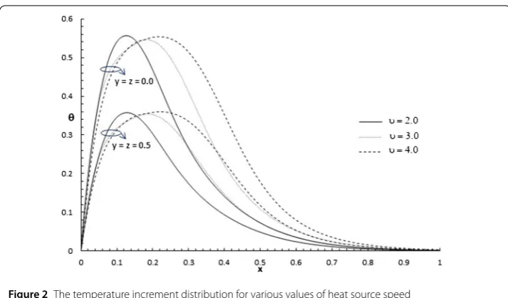
Figure 2The temperature increment distribution for various values of heat source speed
Figure 3The stress distribution for various values of heat source speed
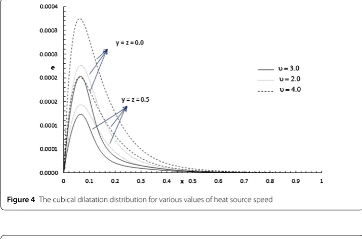
Figures 2–5 represent the temperature increment, stress, strain, and displacement component ux distributions, respectively, for various values of heat source speedυ =
(2.0, 3.0, 4.0) and a wide range of distancex(0≤x≤1) wheny=z= 0.0 andy=z= 0.5 to show the effect of the heat source speed on all the studied functions.
Figure 4The cubical dilatation distribution for various values of heat source speed
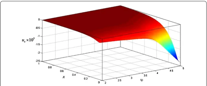
Figure 5The displacement componentuxdistribution for various values of heat source
it separates between the existence of the heat source and its disappearance. The effects of the moving heat source of the current results agree with the results in (Youssef [22–24]; Youssef, Al-Lehaibi [25]).
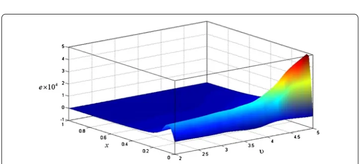
Figures6–9represent the temperature increment, stress, strain, and displacement com-ponentuxdistributions, respectively, for a wide range of heat source speedυand a wide
range of distancexwheny=z= 0.5 to illustrate the effect of the heat source speed on all the studied functions. These figures agree with the results of Figs.2–5.
9 Conclusions
• The value of the speed of the heat source has significant effects on the temperature increment, stress, strain, and displacement distributions.
Figure 6The temperature increment distribution for a wide range of heat source speed wheny=z= 0.5
Figure 7The stress distribution for a wide range of heat source speed wheny=z= 0.5
Figure 8The strain distribution for a wide range of heat source speed wheny=z= 0.5
• The temperature increment, stress, strain, and displacement have different behavior before and after the critical positionx=υt, which separates between the existence of the heat source and its disappearance.
Figure 9The displacement componentuxdistribution for a wide range of heat source speed when
y=z= 0.5
Acknowledgements Not applicable.
Funding
This work has not been supported by any fund from anywhere.
Availability of data and materials
Data sharing is not applicable to this article as no datasets were generated or analyzed during the current study.
Competing interests
The authors declare that they have no competing interests.
Authors’ contributions
HY constructed the problem and the governing equations and advised the co-author on getting the numerical solutions. HY wrote the following sections: abstract, introduction, the basic equation, the formulation of the problem, conclusions, and reviewed all the work. EA solved the problem, applied the Laplace transform on the governing equations and its inversions, prepared figures of the numerical results, and wrote the remaining sections. All authors read and approved the final manuscript.
Author details
1Mathematics Department, Faculty of Education, Alexandria University, Alexandria, Egypt.2Mechanics Department, Faculty of Engineering, Umm Al-Qura University, Makkah, Saudi Arabia.3Mathematics Department, Al-Lith University College, Umm Al-Qura University, Al Lith, Saudi Arabia.
Publisher’s Note
Springer Nature remains neutral with regard to jurisdictional claims in published maps and institutional affiliations.
Received: 4 September 2018 Accepted: 2 January 2019
References
1. Abbas, I.A., Youssef, H.M.: Two-dimensional fractional order generalized thermoelastic porous material. Lat. Am. J. Solids Struct.12(7), 1415–1431 (2015)
2. Danyluk, M., Geubelle, P., Hilton, H.: Two-dimensional dynamic and three-dimensional fracture in viscoelastic materials. Int. J. Solids Struct.35(28–29), 3831–3853 (1998)
3. De Chant, L.: Impulsive displacement of a quasi-linear viscoelastic material through accurate numerical inversion of the Laplace transform. Comput. Math. Appl.43(8–9), 1161–1170 (2002)
4. Duan, R., Liu, H., Zhao, H.: Nonlinear stability of rarefaction waves for the compressible Navier–Stokes equations with large initial perturbation. Trans. Am. Math. Soc.361(1), 453–493 (2009)
5. Ezzat, M.A., Youssef, H.M.: Three-dimensional thermal shock problem of generalized thermoelastic half-space. Appl. Math. Model.34(11), 3608–3622 (2010)
6. Ezzat, M.A., Youssef, H.M.: Two-temperature theory in three-dimensional problem for thermoelastic half space subjected to ramp type heating. Mech. Adv. Mat. Struct.21(4), 293–304 (2014)
7. Ezzat, M.A., Youssef, H.M.: Three-dimensional thermo-viscoelastic material. Mech. Adv. Mat. Struct.23(1), 108–116 (2016)
8. Ghisi, M., Gobbino, M., Haraux, A.: A concrete realization of the slow-fast alternative for a semilinear heat equation with homogeneous Neumann boundary conditions. Adv. Nonlinear Anal.7(3), 375–384 (2018)
10. Marin, M.: An approach of a heat-flux dependent theory for micropolar porous media. Meccanica51(5), 1127–1133 (2016)
11. Mesquita, A., Coda, H.: A boundary element methodology for viscoelastic analysis: part I with cells. Appl. Math. Model.
31(6), 1149–1170 (2007)
12. Morse, P.M., Feshbach, H.: Methods of Theoretical Physics, vol. II (2010)
13. Musii, R.: Equations in stresses for two-and three-dimensional dynamic problems of thermoelasticity in spherical coordinates. Mater. Sci.39(1), 48–53 (2003)
14. Oza, A., Vanderby, R., Lakes, R.S.: Generalized solution for predicting relaxation from creep in soft tissue: application to ligament. Int. J. Mech. Sci.48(6), 662–673 (2006)
15. Parnell, W.J., Nguyen, V.-H., Assier, R., Naili, S., Abrahams, I.D.: Transient thermal mixed boundary value problems in the half-space. SIAM J. Appl. Math.76(3), 845–866 (2016)
16. Podnil’Chuk, I.N., Kirichenko, A.: Thermoelastic deformation of a parabolic cylinder. Vychisl. Prikl. Mat.67, 80–88 (1989) 17. Sarkar, N., Lahiri, A.: Interactions due to moving heat sources in generalized thermoelastic half-space using LS model.
Int. J. Appl. Mech. Eng.18(3), 815–831 (2013)
18. Tahouneh, V., Naei, M.H.: The effect of multi-directional nanocomposite materials on the vibrational response of thick shell panels with finite length and rested on two-parameter elastic foundations. Int. J. Adv. Struct. Eng.8(1), 11–28 (2016)
19. Temel, B., Çalim, F.F., Tütüncü, N.: Quasi-static and dynamic response of viscoelastic helical rods. J. Sound Vib.271(3), 921–935 (2004)
20. Tzou, D.: Macro to Micro Heat Transfer. Taylor & Francis, Washington (1996)
21. Vinogradov, V., Milton, G.: The total creep of viscoelastic composites under hydrostatic or antiplane loading. J. Mech. Phys. Solids53(6), 1248–1279 (2005)
22. Youssef, H.: A two-temperature generalized thermoelastic medium subjected to a moving heat source and ramp-type heating: a state-space approach. J. Mech. Mater. Struct.4(9), 1637–1649 (2010)
23. Youssef, H.M.: Generalized thermoelastic infinite medium with cylindrical cavity subjected to moving heat source. Mech. Res. Commun.36(4), 487–496 (2009)
24. Youssef, H.M.: Two-temperature generalized thermoelastic infinite medium with cylindrical cavity subjected to moving heat source. Arch. Appl. Mech.80(11), 1213–1224 (2010)