R E S E A R C H
Open Access
Context-dependent factored language
models
Gregor Donaj
*and Zdravko Kaˇciˇc
Abstract
The incorporation of grammatical information into speech recognition systems is often used to increase performance in morphologically rich languages. However, this introduces demands for sufficiently large training corpora and proper methods of using the additional information. In this paper, we present a method for building factored language models that use data obtained by morphosyntactic tagging. The models use only relevant factors that help to increase performance and ignore data from other factors, thus also reducing the need for large
morphosyntactically tagged training corpora. Which data is relevant is determined at run-time, based on the current text segment being estimated, i.e., the context. We show that using a context-dependent model in a two-pass recognition algorithm, the overall speech recognition accuracy in a Broadcast News application improved by 1.73% relatively, while simpler models using the same data achieved only 0.07% improvement. We also present a more detailed error analysis based on lexical features, comparing first-pass and second-pass results.
Keywords: Speech recognition, Factored language model, Dynamic backoff path, Word context, Inflectional language, Morphosyntactic tags
1 Introduction
Speech recognition still performs poorly in inflec-tional languages compared to mainstream languages like English. The cause can be found in the rich morphology of such languages, which increases the need for larger vocab-ularies. It is estimated that inflectional languages need up to ten times larger vocabularies than English [1, 2].
Although we can easily build larger vocabularies, thus reducing the number of recognition errors caused by out-of-vocabulary words, the use of such models increases not only the size of language models but also the required size of training corpora. With larger vocabularies, words are also substituted more easily, especially if they are acous-tically similar. Many errors occur only in the grammatical sense, when a recognition error results in a word with the same lemma but with a grammatical error, e.g., a false case or number.
An often used approach in speech recognition of mor-phologically rich languages is the incorporation of gram-matical information in some form. One practical imple-mentation to achieve this is the use of a factored language
*Correspondence: [email protected]
Faculty of Electrical Engineering and Computer Science, University of Maribor, Smetanova ul. 17, SI-2000, Maribor, Slovenia
model (FLM). Such models were first proposed for speech recognition in Arabic languages [3], but they have also been adopted in statistical machine translation [4] and, more recently, in natural language generation [5].
In an FLM, each word is represented as a vector of fac-tors containing information about the word. One of the factors is usually the word itself; other factors can be the lemma, the morphosyntactic description (MSD) tag, the word stem, the ending, the root, etc. While traditional (word-based)n-gram language models use only the basic word forms to estimate the probabilities of sentences, FLMs can use all defined factors and their information. Since these factors have fewer possible values (smaller vocabularies), we can build simple models on individual factors using smaller training corpora.
The idea of FLMs, however, is to use different factors in the same models. As each word can have several factors, such an FLM will have many more terms in its condi-tional probability than tradicondi-tional n-gram models or an FLM using only one factor. The potentially large num-ber of selected factors again increases the need for larger training corpora, which may not be available for some languages or applications, causing data sparsity problems.
The two important steps for defining an FLM are to define a set of relevant factors and to define the back-off path, which determines the order in which to discard factors in the case of training data sparsity.
In the present paper, we propose a novel approach to factor definition and backoff path selection for FLMs, in which the model considers only specific factors from spe-cific words that can improve recognition performance. The selection of these factors and their order in the backoff path is made dynamically, based on the parts of speech of words in the current context. Thus, the name is context-dependent FLMs. With this approach, we can build FLMs with a limited number of factors in each prob-ability estimation, which can improve recognition perfor-mance while avoiding new data sparsity problems. This method also makes use of grammatical properties of the target language, as the process of determining the backoff path searches for specific correlations in a given sentence structure.
1.1 Previous work
The first results on FLMs were perplexity calculations, e.g., on the Arabic Callhome corpus [6] or the Wall Street Journal corpus [7]. In both studies, the authors reported perplexity improvements. Later, the models were used in speech recognition applications [3].
While a backoff path can be selected manually and may remain fixed, the authors of FLMs proposed several methods for determining the backoff path based on train-ing data, e.g., the (normalized) number of occurrences and the maximum probability of the vertex. One of these methods—min/max counts—was used by the authors in [8]. The authors in [7] also proposed to using several back-off paths simultaneously and determining the set of those paths in run-time.
FLMs are often used in Arabic and Slavic languages, probably most prominently in Russian [9, 10], as well as in other morphologically rich languages such as Romanian [8], Turkish [11], and Amharic [12].
There is previous work with N-best list rescoring
using FLMs. In [13], the authors presented an N-best
list rescoring approach in which the language model was adapted based on the vocabulary in the hypothe-sis list. While the system used morpheme-based mod-els in the first pass, the performance improved in the second pass, in which the models were word based. Part of the difference between the first and second pass can be explained with the use of trigram sub-based models in the first pass and the trigram word-based models in the second pass. It was shown that sub-word-based models require higher model orders to achieve performance comparable with word-based mod-els [14]. The authors in [15] implemented FLMs with the use of morpheme units for language modeling. With
N-best list rescoring, they achieved an improvement of 0.3% absolutely.
Sak [11] showed for the Turkish language that the improvements achieved by using FLMs rather than tra-ditional n-gram models are greater while only limited size corpora are available for training; the improvements decreased as the corpus size increased. These results can be considered relevant to speech recognition in specific domains with limited training data, where data sparsity becomes a problem for word-based models.
In [16], the authors defined trigger part-of-speech (POS) tags and used them as syntactic features, demonstrat-ing that FLMs can outperform traditional trigram lan-guage models regarding perplexity and mixed error rate in speech recognition. While their approach included POS tags, the backoff paths were selected based on overall perplexity.
In previous research, backoff path selection is often made with fixed backoff paths, a method based onn-gram occurrences in training data, or overall perplexity results on development data. Our approach differs from previ-ous work as we perform backoff path selection for each word sequence individually in run-time, selecting the path differently for each possible sequence of POS tags in the context and basing the decision on the perplexity results relevant only to the considered sequence of POS tags.
1.2 Structure of the paper
In Section 2, we present the basics of FLMs required for an understanding of the proposed context-dependent FLMs and their implementation. In Section 3, we present our proposed models along with all of the algorithms neces-sary to efficiently determine backoff path selection, and, in Section 4, a two-pass recognition algorithm suitable for using the proposed models is introduced. In Section 5, we describe our experimental system used for building and testing the models. The obtained results are then presented in Section 6, followed by the conclusion in Section 7.
2 Morphosyntactic description tags
A basic process of text or speech annotation is the addi-tion of part-of-speech (POS) tags to each word in a text. The most basic tags would be noun, adjective, verb, adverb . . . residual. However, to be more useful, typically addi-tional properties are considered. Tags which hold more information, especially in morphologically rich languages, are called morphosyntactic description (MDS) tags.
For example, Penn Treebank Project specifies 36 dif-ferent POS tags for the English language. Some part of speech have several possible tags, e.g., there are four different nouns listed with tags in parentheses:
• Proper noun, singular (NP) • Proper noun, plural (NPS)
These tags are used by TreeTagger, a freely available MSD tagger for several languages.
As English is not a morphologically complex language, its POS tags give only sparse information on the gram-matical role of a word in a sentence. Typically, information that is given by POS tags is the number for nouns (singular or plural) and some information about verbs (base form, past tense, present participle, third person, etc.).
In the MULTEXT-east project [17], tagsets for sev-eral languages were specified and standardized includ-ing a more complex tagset for English. Version 5 of the project specifies 16 categories (parts of speech) with a total of 31 attributes and a set of 135 different tags. For example, verbs have the following attributes: type, verb form, tense, person, and number, and the attribute person has the following possible values: first, second, and third.
Slovene, being morphologically complex language, has much more different tags. The JOS specifications [18], which were derived from the MULTEXT-east system, define 12 parts of speech. Again, some parts of speech have several attributes, e.g., verbs have the following attributes: type, aspect, form, person, number, gender, and negative. Some parts of speech have none additional attributes, e.g., particles and interjections. JOS specifies 12 parts of speech with a total of 37 attributes and a set of 1902 different tags.
Considering all possible values for all attributes of a given part of speech and all parts of speech, JOS defines 1902 different MSD tags for Slovene.
Figure 1 shows a Slovene sentence with part of speech tags. The set was annotated with Obeliks, a tagger for Slovene. The text is in XML-TEI format and is also tagged with lemmas. A translation of the sentence into English is tagged in Fig. 2. The translation was tagged with TreeTag-ger and result converted into the same XML-TEI format. The sentence was taken from the BNSI test set, later used in this research.
Fig. 1An MSD-annotated text in Slovene
Fig. 2An MSD-annotated text in English
3 Factored language models
Language models are used to estimate the probability of a given word sequence W = (w1,w2,. . .,wn). Most
commonly used are traditional word-basedn-gram
lan-guage models, which estimate the conditional probability of each word given the previousn−1 words. The current and previous words in these models are often called the context.
In an FLM, each wordwis represented as a vector ofK
factorswi =
fi1,fi2,. . .,fiK, whereiis the index number
of the word. Much like in word-basedn-gram language
models, the probability of a sentence is the product of the probabilities of individual words. In the case of an FLM, we use the conditional probabilities of all factors in the estimated word given the factors of previous words:
Pfi1:K|fi1:K−1,fi−1:K2,. . .,fi1:K−n+1. (1)
Using the chain rule for probabilities, we can express this probability with
P
fi1:K
=
K
k=1
P
fik|fi1:k−1,fi−1:K1,. . .,fi1:K−n+1
. (2)
The probabilities of individual factors on the right-hand side are again conditional probabilities given the factors from previous words and previous factors from the cur-rent word. With several words of history and several factors per word, the total number of given factors can quickly exceed a feasible amount for practical application.
Similarly, in word-based n-gram models, the above
equation also makes use of data from sequences of n
words so that we can speak of ann-gram FLM. We say that
nis the FLM order. We also use this definition of the FLM order when only some of the possible factors are present in the conditional probability.
probability and back off to a model with fewer terms. If necessary, we can repeat the process to reduce the num-ber of terms further. The selection of a backoff path in a word-basedn-gram model is rather clear: on each step, we discard the most distant word, based on the assumption that more distant words have less impact on the current word. However, in an FLM, several factors can have the same distance from the current factor. Furthermore, there is no guarantee that discarding one of the most distant factors will result in better performance than discarding some closer factor, whether it is the same type of factor or not.
Often, lemmatizers and MSD taggers are used as tools to automatically determine grammatical properties. In this case, it is important that we try to identify all of the fac-tors with the potential to improve performance in the application and include only those factors in the model. While other factors may not decrease performance, they will increase the size of the model and make the final application more time and space consuming.
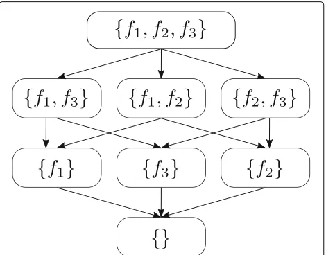
In the context of FLMs, the backoff path first became relevant and the backoff graph was introduced. We can define the backoff path as a sequence of factor subsets. On every step in the backoff procedure, we move to another subset that has one factor less than the previous subset. The selection of the factor to be removed at each step determines the backoff path. Assuming we havekfactors as the conditional terms in the FLM probability, we start with the set of all factors. On every step, we discard one factor that is still in the path. This method gives usk! pos-sible backoff paths. Figure 3 shows a backoff graph that illustrates this principle in the case of three factors. The vertices of the directed graph represent subsets of factors used in the conditional probability.
Fig. 3Backoff graph for an FLM with three factors
4 The context-dependent backoff path
In the proposed models, we will use run-time determi-nation of the backoff path, although we will use only one path simultaneously. Backoff path determination will be achieved using POS information from the currently esti-mated word sequence. We have therefore called these backoff paths and models context-dependent. We will later define the backoff function, which will tell us which path to use for probability estimation, given the current word and its context.
We based the proposed models on the property of gram-matical matching in inflectional languages, in which the properties of some words correlate with the properties of other words. An example is the matching of case, num-ber, and gender between nouns and adjectives. Given that these words might not be adjacent in the sentence, we made the assumption that it is not always best to discard more distant factors; examining which parts of speech are present in the sentence might suggest which factors are better suited for probability estimation.
The first step in building the proposed language models is to determine the set of different factors for each word. We found that word-basedn-gram language models still have the greatest impact on performance. Thus, one fac-tor shall remain the word itself. Other facfac-tors can be the lemma and grammatical properties, either as separated factors or combined (e.g., MSD tag). We can also include other information if it is useful and if appropriate tools are available to determine it automatically.
One necessary piece of information in the proposed models is the POS tag, which can be incorporated as a separate factor or can be included within the MSD tag.
4.1 The backoff function
LetPidenote the POS tag of wordwi. Assuming we have an input word sequence(wi−n+1,. . .,wi), we can deter-mine a corresponding POS sequence(Pi−n+1,. . .,Pi). We then define the backoff function
BO :(Pi−n+1,. . .,Pi)→(f1,. . .,fl), (3)
for every possible POS sequence, where(f1,. . .,fl)is an ordered set of factors to be included in the conditional probability (Eq. 2). While the set alone defines the start-ing point in the backoff graph, its order determines the backoff path. Considering the above equation, we will start withlfactors and then remove them one by one from right to left.
Let us assume that for each word, we have definedK
factors and we are considering a model of ordern. The conditional probability will have betweenK·(n−1)and
and stop-of-sentence tags. We can derive the total number of valid POS sequences of lengthn≥2 as:
(|P| −1)2·(|P| −2)n−2. (4) For a sequence to be valid, the start-of-sentence tag can appear only in the first place and the end-of-sentence tag can appear only in the last place, while all other tags are not restricted.
Factor probabilities can be expressed conditionally given the factors of previous words and the previous fac-tors of the current word. If we are currently considering factork, the number of possible conditional factorsmis
m=(n−1)·K+k−1. (5)
If we were to look for backoff paths that start with a set of all possible factors, the number of backoff paths would be
m!. For shorter paths of lengthl, the number of possible backoff paths is
m!
(m−l)!. (6)
Finally, the number of paths of all possible lengths is m
l=0
m!
(m−l)! , (7)
where we also include a path of length 0, which is a model containing only the modeled factor itself and no conditional factors.
Depending on the number of possible POS tags and the model order, the number of different POS sequences can increase beyond a feasible amount. The number of all pos-sible paths increases even faster, exceeding 108for trigram models with three factors, for example. Therefore, it is necessary to implement an efficient method to determine the backoff function BO.
4.2 Initial algorithm
Let us first assume that we have the necessary equipment to consider the whole search space and a training set large enough to train all models. A simple brute-force search to determine backoff paths is presented in Algorithm 1, whereNis the maximal model order,Kis the number of factors in a word, and Pn is the set of all possible POS sequences of lengthn.
The final output of the algorithm is one backoff pathMˆ
for each possible POS sequence, given the model order and the factor to be estimated. The algorithm works by testing all possible paths M and selecting the path that maximizes a certain functionT. We need to repeat the algorithm for different model orders and all defined factors.
Let us consider the computational complexity of the
initial algorithm. The maximum model orderN and the
number of factors per wordK are given. The number of
Algorithm 1:Initial brute-force algorithm for backoff path determination.
Input:N Input:K
Input:Pn ∀n∈ {1,. . .,N} Output:S
begin S = ∅
forn∈1,. . .,Ndo fork∈1,. . .,Kdo
forP∈Pndo ˆ
M←−No solution
forM∈Mdo
ifT(M) >T(Mˆ)then ˆ
M=M
S←−S∪(n,k,P,Mˆ)
possible POS sequencesPnis given in Eq. 4, as a function of the number of different POS tags|P|. The number of all paths of the maximum given lengthlis given in Eq. 7. Con-sidering the nested loops in Algorithm 1, the total number of models to be trained and tested can be expressed as
N
n=1 K
k=1
(|P| −1)2(|P| −2)n−2 m!
(m−l)! , (8)
wheremis described in Eq. 5.
The number of possible POS sequences can be ignored when we are interested in the umber of models to be trained and tested, since models can be reused for any POS sequence, and results can be filtered accordingly to the actual POS sequence. In any case, we can then derive the computational complexity of the brute-force algorithm as
O(|P|N(NK)(NK)). (9)
Clearly, this algorithm is not tractable and we shall, there-fore, derive a feasible system.
However, the presented algorithm will be the starting point from which we will derive a feasible system. In order to achieve this, we have to address several issues
1. Determine a criterion functionT that will be fast and will have the ability to estimate the performance of models. The criterion function is needed to estimate which model will perform better in the final
application.
searching. Such a list is essential as a search through all possible paths would not be feasible.
3. Define a method to combine different POS sequences, as the training data for some individual sequences would be too small for obtaining a reliable probability estimate.
4.3 Criterion function
In order to determine a language model’s performance, we could use it in the final application, in our case speech recognition. This will provide the best estimate of whether a particular model will outperform another model or not. This method is only feasible if we test just a handful of models. However, this does not apply to our case.
We often estimate the performance of a model by cal-culating its perplexity on a selected development text. Compared to estimation within speech recognition, this method is much faster, as we only need to estimate each sentence once. Furthermore, it has been shown that there is a correlation between a language model’s perplexity and its performance in speech recognition [20].
In the presented algorithm, we want to compare mod-els with different backoff paths. While the perplexity of a model is typically estimated using the whole text, we now want this estimate only at words with the given context.
The backoff path selection for each word will be inde-pendent of the backoff path selection at neighboring words and so the contributions of individual words to the perplexity of the whole text will also be independent. Thus, we can use perplexity and slightly modify its calcu-lation for use as our criterion function. This modification will be necessary as we need to compare models not on the whole text but only at words with a given context.
The perplexity PP of a modelMon a textWis defined by
PPM(W)=2HM(W), (10)
whereHM(W)is the cross entropy
HP(W)= 1
−T ·log2P(W)
= 1 −T ·log2
T
i=1
P(wi)
, (11)
whereTis the total length of the text.
We want to modify the perplexity definition to our needs. LetP∗denotes a given POS sequence. For eachP∗, we define a set of numbers
I(P∗)⊂ {1,. . .,T}, (12)
containing indexes of words with the POS contextP∗:
i∈I(P∗) ⇐⇒ (Pi−n,. . .,Pi)=P∗. (13)
We can then define a modified cross entropy on the subset of corresponding words as
H∗(W,P∗)= 1
−|I(P∗)|log2
i∈I(P∗)
P(wi). (14)
For our criterion function, we can then use the modified perplexity
PP∗(W,P∗)=2H∗(W,P∗). (15)
We shall note that better models have a lower perplex-ity, and we can decide either to minimise the criterion function or to use the negative value of the perplexity as a criterion functionTand maximize it. In the present paper, we will use the latter approach.
4.4 Backoff path lists
We derived a search algorithm that will build a list of back-off paths to be tested considering the following guidelines:
1. Up to a certain length, it is still feasible to test all possible paths, and we shall do so. We can build longer paths by extending the best shorter paths. 2. We will use a beam width, a technique used by
speech recognition search algorithms to exclude less likely hypotheses. As in these recognition search algorithms, we will keep a list of possible paths and exclude candidates that have results (obtained by the criterion function) that fall sufficiently below the current best path.
3. If a certain path is given, we will search for additional factors considering the factors from the next word back not only in the current word’s history but also in several words of history.
The backoff path search Algorithm 2 takes the cur-rent list as input and gives a new list of backoff paths as output. For each path in the input list, the algorithm deter-mines all possible factorsF∗with which the path can be expanded. After we include these new paths in the list, the algorithm tests them with the criterion function and finds the best backoff pathM∗. Finally, a beam widthε is determined and all paths falling outside the beam are discarded.
The search algorithm must be repeatedm-times, where
mis the maximum number of factors allowed in a path,
as the algorithm always creates paths that are one factor longer than the input paths. However, the algorithm is not employed for short paths, as the list is generated with all possible paths. The final result is a list of backoff paths of lengthmor shorter.
The beam width ε is empirically determined for each
Algorithm 2:The search algorithm for determining a list of backoff paths for a given POS sequence or POS class.
Input:M Output:M∗ begin
M∗=M
for∀M∈Mdo DetermineF∗ for∀F∈F∗do
M∗=M∗∪ {(M+F)} ˆ
M∗=arg max M∗∈M∗ T(M
∗)
Determineε
for∀M∗∈M∗do
ifT(M∗)≤T(Mˆ)−εthen M∗=M∗\ {(M)}
larger change of perplexity than in longer paths. If we expand shorter paths with a certain difference in perfor-mance with additional factors, the worse performing path has a greater chance of being expanded into a path that will later outperform other paths.
The described search algorithm is executed for a given class of POS sequences, and it must be repeated for every class. These classes will be defined in the next section.
4.5 POS sequence classes
Due to the large number of POS sequences, data spar-sity will become inevitable. We decided to group POS sequences into a smaller number of classes based on their similarity. Each class will consist of one or more POS sequences, and the final application will make use of a backoff path assigned to the class containing a certain POS sequence. Thus, the criterion function and the search algorithm described above will be performed using classes of POS sequences.
Given that the primary problem leading to the need for POS classes is data sparsity for some POS sequences, we decided that the algorithm shall merge the POS class with the smallest number of occurrences in the training set with the most similar POS class. The final result shall be a set of POS classes that all have a sufficient number of occurrences and contain similar POS sequences. The algorithm takes a set of classes as input and returns a smaller set of classes as output.
We define the first set of classes with one set for each POS sequence that has occurred. The merging algorithm then performs several iterations to reduce the number of classes until it reaches the outer loop threshold α.
In these iterations, we first determine a list of possible backoff paths for each class using the search algorithm described above. We then perform several iterations of class merging, where the class with the smallest number of occurrencesP¯is merged with the most similar classP¯. For this purpose, we need to define the similarity function
D. We repeat the merging until the number of classes falls below the inner loop thresholdβ.
The similarity between two classes is based on the two obtained lists of backoff paths. We look for a backoff path that gives good (but not necessarily the best) results in both classes. When faced with a small number of occur-rences, we can also incorporate the POS sequences them-selves to determine the similarity of classes. Other infor-mation can also be included to determine the similarity between classes.
The algorithm was conceived with two nested loops. The outer loop determines the final number of classes and incorporates the inner loop for a trade-off between speed and reliability. We might assume that if two classes are similar, they will also be similar to the merged class. We do not assume that after several iterations, merged classes will still behave similar to the original classes from which they were merged; we therefore incorporated an inner loop that determines how many merging iterations we want to perform before determining new backoff path lists for the merged classes.
Algorithm 3:The merging algorithm, used for merg-ing different POS classes based on their similarity.
Input:P Output:P∗
Output:M(P¯) ∀¯P∈P∗ begin
P∗=P
Determineα
repeat
for∀¯P∈P∗do DetermineM(P¯)
Determineβ
repeat ¯
P=arg min
¯
P∈P |( ¯ P)| ¯
P= arg min
¯
P∈P\{P¯}
D(P¯,P¯)
P∗←MergeP¯andP¯
until No. classes< β untilNo. classes< α
4.6 Final path selection
algorithm. The output will again be a list of different back-off paths. For the final solution, one of them must be selected.
One simple solution would be to choose the model with the smallest perplexity, regardless of other considerations. However, we can compare the models by their perplexity as well as their size. We are therefore able to make a trade-off between the expected results and the expected speed of the models.
We propose a simple algorithm to select another model, where we first consider smaller models that would esti-mate probabilities faster. We first choose the smallest model. We then test all other models in ascending order of model size. If a larger model has a lower result of the criterion functionT (i.e., higher perplexity), we skip it. If a larger model has a significantly higher result of the crite-rion function, we select this model as our current choice.
We need to determine a threshold γ that defines how
much better the result of the criterion function must be in order to call it significant.
We do not want to select a significantly larger model if the criterion function increases only by a minimal amount; however, we still want to allow the possibility of choosing a slightly larger model. Therefore, we allowed the selection of a larger model if the criterion function gives a better result and the model’s size increases by an amount smaller than the thresholdδ.
The process of selecting the final model is represented in Algorithm 4. We are again forced to determine two heuris-tic constants:γ andδ. We can start by settingγ = 0 and
δ = ∞so that the algorithm will give us the model with the best criterion function result. We can then change the values of both constants to achieve a compromise between performance and speed.
Algorithm 4:The selection algorithm, used to deter-mine which model from the solution set will be used in training and recognition.
Input:M Output:Mˆ begin
SortMby size
ˆ
M←−find smallest model inM
for∀M∈Mdo Determineγ inδ
if(|M|>| ˆM| & T(M) <T(Mˆ)then Next
ifT(M) >T(Mˆ)+γ then ˆ
M←−M
ifT(M) >T(Mˆ) & |M|<| ˆM| +δthen ˆ
M←−M
4.7 Model usage
Our final result obtained by the selection algorithm is the backoff function. This function is determined for each model order and each defined factor. While using a context-dependent FLM for a given word sequence, we decide which model order we want to use. Usually, it would be the largest order available, except at the begin-nings of speech segments, where there are fewer words in the context. We then determine the POS sequence and look up the POS class in which this sequence has been merged. For each factor, we find the selected path for this function and then calculate estimates using these backoff paths.
5 The recognition algorithm
An appropriate system for testing the performance of context-dependent models is a two-pass continuous speech recognition algorithm.
In the first recognition pass, we typically make use of acoustic models and word-based language models. The main requirement of the speech recognition search algo-rithm is that it will produce a list of hypotheses for each speech segment. In the first pass, each hypothesisW is scored with the equation
P(W)=pAPA(W)+pLPL(W)+pIC(W), (16)
wherePAandPLare probabilities obtained with an acous-tic and a word-based language model, respectively.
Func-tion C is a simple word count function. We call these
results the individual scores. Coefficients pA,pL, andpI are the acoustic model weight, the language model weight, and the word insertion penalty, respectively.
We then use an MSD tagger to annotate the hypotheses with all information used in the context-dependent FLMs. In order to reduce the space requirement for the hypothe-ses, we shall include only useful information, e.g., we can discard information produced by MSD taggers, which will not be used by the models.
In the second recognition pass, the hypotheses are rescored. We can use all three scores from the first pass and add scores from context-dependent FLMs. For exam-ple, if we have three factors, i.e., three FLMs, the scoring function becomes
P(W)=pAPA(W)+pLPL(W)+pIC(W)
+p1Pf1(W)+p2Pf2(W)+p3Pf3(W), (17)
wherePf1(W),Pf2(W), andPf3(W)are probability scores obtained by the three context-dependent FLMs. Each of these three scores also has an appropriate weight:p1,p2, andp3.
acoustic model weight to 1 and we use an optimization algorithm for the remaining weights.
We perform several recognition run-throughs on the development set to find the best language model weight and word insertion penalty for the first recognition pass. We then use the optimized values in a single recognition run-through on the evaluation set.
In the second pass, we use lists of N-best hypothe-ses from both the development and the evaluation sets. We optimized all model weights and the word insertion penalty again on the development set and used them in the evaluation set.
A brute-force exhaustive search of optimal values would again not be feasible, as we have several real-valued val-ues to optimize. Two weights are already present in the first pass but need to be optimized again. For each fac-tor in the context-dependent FLMs, we have an additional weight to optimize. A simple algorithm was devised to optimize these weights. The algorithm works onN-best lists of all hypotheses in the development set. It starts with an initial set of values for all weights and then optimizes only one weight at a time while all other weights remain constant, before moving on to the next weight. The algo-rithm performs several iterations of optimizing all weights for a predefined number of times or until the optimized values do not differ from the values obtained in the previ-ous iteration. We can repeat the algorithm with different starting values.
6 Experimental system
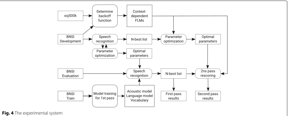
We evaluated the performance of the proposed language models on a large vocabulary continuous speech recogni-tion (LVCSR) applicarecogni-tion in an inflective language, namely a Slovene Broadcast News transcription. The general structure of our system is presented in Fig. 4.
6.1 Speech databases
The Slovene Broadcast News (BNSI) database [21] was the only speech database used; it is also the only Slovene speech database appropriate for LVCSR. It consists of approximately 25 h of transcribed speech data. The largest part serves for acoustic model training, while the rest makes up the development set and the evaluation set, each consisting of approximately 2.5 h of speech data. We used the development set in all parameter optimization pro-cesses and the evaluation set for obtaining recognition results.
We trained word-basedn-gram language models on the 620 million words FidaPLUS corpus of the Slovene lan-guage [22], which consists mainly of articles from newspa-pers and journals. While it is available in a lemmatized and MSD-tagged form, we used only basic word forms from it. The Slovene ssj500k corpus is a manually MSD-tagged and lemmatized corpus consisting of approxi-mately 500,000 words. We used it for the training of all FLMs. It is large enough to effectively train models with a limited vocabulary—in this case POS tags and MSD tags.
The MSD tags in the ssj500k corpus follow the JOS specifications [18], which themselves were derived from the MULTEXT-EAST system [17]. Depending on the POS tags, the MSD tags can hold several grammatical cate-gories. However, we found that only a few are useful in the presented application: POS, type, gender, case, number, and person. All other tags were removed.
6.2 First pass
The speech database was manually segmented. The trained acoustic models were HMM triphones with 16 Gaussian mixtures. We used 39 features of mel-frequency cepstral coefficients (MFCC): energy features and 12 fea-tures with delta and delta-delta coefficients.
The vocabularies in the first pass include the most common words in the FidaPLUS corpus. We built vocabu-laries ranging from 60,000 to 300,000 words, constructing bigram and trigram models on all vocabulary sizes. Two smoothing techniques were used: Good-Turing and mod-ified Knesser-Ney.
In the first pass, we used a Viterbi decoder to obtain an N-best list for the development and evaluation sets (N = 1000). We repeated the recognition on the devel-opment set in order to obtain optimal parameters for the language model weight and the word insertion penalty and used the optimized values on the evaluation set. We used the Obeliks tagger—an MSD tagger developed especially for the Slovene language—on allN-best lists.
6.3 Context-dependent model training
The first step in building context-dependent models was to define factors. The Obeliks tagger generates tags according to the JOS specifications, in which 12 different POS tags are defined, some of them having different types. Combining the POS tag and type, we defined an extended
POS tag, e.g., we distinguished the types common noun
andproper nameinstead of usingnoun. We decided to use extended POS tags due to grammatical concerns, as dif-ferent types of the same part of speech can have difdif-ferent grammatical properties. The extended POS tags had 32 possible values. According to the search space estimation in the previous section, we have a total number of over one billion possible POS sequences with lengths up to six. Next, we built MSD tags that included only gender, case, number, and person. Preliminary experiments showed that those grammatical categories could improve perfor-mance in speech recognition, while other grammatical categories cannot. We therefore used a reduced MSD tag set. Different parts of speech can have from 1 to 255 differ-ent values of the reduced MSD tag. The last chosen factor was the word itself.
We trained all MSD models on the ssj500k corpus. Not all possible POS sequences appeared in the corpus. For the first determination of POS sequence classes, we used only those sequences that did appear in the corpus. In Table 1, the number of classes depending on the model order is shown. The numbers are significantly lower than the theoretical upper limit, as most theoretically possible sequences do not produce meaningful or grammatically sensible sentences.
While implementing all of the necessary algorithms to determine the backoff function, we had to determine sev-eral heuristic constants. We did this experimentally to achieve good performance with reasonable time and space demands. The beam width ε itself is newer fixed but is rather determined based on the currently best hypothe-ses in the search algorithm and the number of factors already in the backoff path, e.g., if the path has perplexity
Table 1Number of POS classes given the model ordern
observed in training and used for the first determination of POS classes
n Number of sequences
1 30
2 475
3 3003
4 8666
5 13,682
6 15,478
PPminand a certain number of factors, the beam width is determined as
ε=PPmin·Fε, (18)
where values for Fε are given in Table 2. Any backoff
path with a perplexity higher than PPmin + ε will be
discarded. Additionally, we implemented further criteria in the pruning procedure. If the set of possible backoff paths contains two paths that contain the same factors in a different order, we excluded the worse performing model. We found that the search algorithm time demands changed by about 10%, when using different values of the factors in Table 2 ranging from 0.1 to 2 at all path lengths and, therefore, different values forε. Finally, the values in Table 2 were chosen based on preliminary results obtained during the implementation of the search algorithm.
Unlike ε, the thresholdsα andβ in the merging algo-rithm have almost no impact on the time demands in determining the backoff function.
We determined α = 10 for unigram models and
α = 50 for higher order models to be suitable values. The parameterβis determined in each iteration at run-time. We added the constraint that the number of classes in the inner loop must not be reduced by more than 50%.
Lastly, we had to determine the parametersγ andδin the selection algorithm. Those parameters have no effect on time demands for training. It was also found that they do not have a significant impact on model performance. We chose γ to be 5% of the perplexity of the currently
Table 2Pruning width factorskfor the search algorithm given the number of factors
No. factors Fε
1 1.0
2 0.5
3 0.3
4 0.2
selected model andδto be 25% of the size of the currently selected model in terms of entries in the language model.
6.4 Computational demands
The total time to perform the search algorithm was 56 h, of which the largest part (36 h) was spend using model
order n = 5. It was performed on a dual-processor
server with 88 logical threads at 3.6 GHz and 128 GB of memory. We shall note that the exact time depends not only on hardware configuration but also on software, other server load, development and training sets, and the possibility of parallel processing. We also reused already build models.
Rather than comparing real-time values, we shall state the number of trained models. Table 3 shows the num-ber of all possible backoff paths given the model ordern
and the current factork. The number of maximum
mod-els is based on Eq. 5; however, we also limited the backoff path length to eight factors. We also show the number of models that were actually trained and tested with our final search algorithm. We see that at higher model order, the number of tested models only slightly increases, while the number of maximum models reaches infeasible numbers. The final ratio between the sum of all tested and sum of all possible models is 1:1100. This means that we tested 1100 times fewer models than we would have to in brute force. Even, if we consider models with an order of up to 4, this ratio would be 1:200.
Table 3Comparison of the number of all possible backoff paths with the number of trained and tested paths with regard to model ordernand modeled factork
n k Maximum Tested
1 1 1 0
1 2 2 1
1 3 5 4
2 1 16 15
2 2 65 55
2 3 326 176
3 1 1957 705
3 2 13,700 1758
3 3 109,601 5129
4 1 623,530 15,320
4 2 2.61×10⁶ 15,505
4 3 8.71×10⁶ 21,552
5 1 2.47×10⁷ 56,888
5 2 6.19×10⁷ 45,085
5 3 1.41×10⁸ 51,466
Total 2.40×10⁸ 213,659
It should be noted that one possibility is a model without any factors. This model was not tested as it always gives the lowest performance. Therefore, the number of all pos-sible backoff paths in the table is 1 higher than the number of tested models at data points where otherwise all models were tested.
6.5 Simple MSD models
In order to determine whether the context-dependent backoff paths have any effect on the recognition perfor-mance that is not due to the inclusion of MSD data itself, we also built simple language models based on MSD tags. These models are based on the extended POS tag (P) and the MSD tag (M).
The first set of models is defined by
P(P0|P−1,. . .,P−n),
P(M0|M−1,. . .,M−n).
(19)
The backoff path in both models is to remove the most distant factor. In the first set, we only use factors of the same type in the model. These models aren-gram models
of extended POS tags and n-gram models of MSD tags.
The second set of models is defined by
P(P0|P−1,. . .,P−n,M0,. . .,M−n),
P(M0|M−1,. . .,M−n,P−1,. . .,P−n).
(20)
Here, both types of factors are used in the same model. We built models with a maximum of seven conditional factors and considered at most five words of history. Therefore, we obtained 6-gram FLMs with fixed backoff paths of no more than eight vertices. The limits of the number of factors and history length are due to preliminary results indicating that longer paths are of no further benefit to the performance. Additionally, we added the constraint that if a particular factor appears in these models, then all fac-tors of the same type that are closer to the modeled word must also appear.
Backoff paths are built simply by adding one of two possible next factors to the path. A total of 244 possible models were built, all with backoff paths that comply with the presented constraints.
These models were later used to obtain results regarding the degree to which performance can be improved if morphological information is introduced into the speech recognition algorithm without introducing context-dependent models.
6.6 Tools
determination and the second recognition pass, tools were developed within the framework of the present research.
7 Results
7.1 First pass andN-best lists
Table 4 shows recognition results in word error rate (WER) for the first recognition pass with bigram and tri-gram language models with Good-Turing and modified Knesser-Ney smoothing and different vocabulary sizes. Vocabulary size and model order have an expected impact on performance. However, while other research indicated that modified Knesser-Ney smoothing performs better than Good-Turing [24], our results show the opposite, although there are only slight, statistically non-significant differences. The best WER result of 22.64% was obtained with a trigram Good-Turing smoothed model built on a 300K vocabulary. Similar results can be obtained on the BNSI development set.
We can also compare computational and memory con-sumption. Table 5 shows real-time factors (RTF) for all first-pass scenarios. We notice only small differences with regard to the smoothing method. Results show that RTF increases by a factor of 2 if the vocabulary size is increased from 60K to 300K and by a factor of 3 if when using tri-gram models compared to bitri-gram models. Considering also recognition results, we see that the increase in vocab-ulary brought a larger performance increase with a smaller RTF increase than the increase in model order.
However, increasing the vocabulary size mainly elim-inates errors due to out-of-vocabulary words. With the 300K vocabulary, the out-of-vocabulary rate is 1.02% and further enlargement of the vocabulary results in only small recognition improvements.
Preliminary research showed us that there are also only small differences in model perplexity if we increase the model order to 4-gram models. Also, the recognition results we found increase only slightly if at all. This was found using a two-pass rescoring algorithm as the recog-nition tool (HDecode) supports only bigram and trigram models.
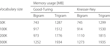
Table 6 shows us the the memory demands for all first-pass scenarios. We can again observe that increase in
Table 4Recognition results in the first pass obtained on the BNSI evaluation set
Vocabulary size
WER [%]
Good-Turing Knesser-Ney
Bigram Trigram Bigram Trigram
60K 33.89 30.73 33.84 30.95
100K 31.27 28.08 31.24 28.36
200K 29.70 26.27 29.78 26.53
300K 29.22 25.64 29.28 25.87
Table 5Average real-time factors for recognition in the first pass obtained on the BNSI evaluation set
Vocabulary size
Real-time factor
Good-Turing Knesser-Ney
Bigram Trigram Bigram Trigram
60K 6.29 18.46 6.14 18.62
100K 7.82 23.42 7.52 23.37
200K 10.44 31.55 10.48 31.71
300K 12.66 37.09 12.88 37.70
vocabulary size increases the memory demands slightly less than the increase in model order.
We have to add that the exact values for RTF as well as memory consumption depended on the computer hard-ware and the softhard-ware tools used.
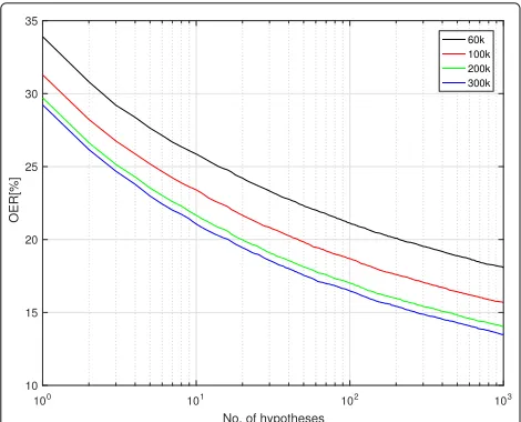
When rescoring theN-best list, there is always an upper limit of how much improvement can be achieved, as only a limited number of hypotheses are available in the sec-ond pass. Assuming we had a system in the secsec-ond pass that would always select the best hypothesis (an oracle), we would still have an error rate—the so-called oracle error rate (OER)—that is dependent on the number of hypotheses. The OER results on the BNSI evaluation set using bigram and trigram language Good-Turing mod-els are shown in Figs. 5 and 6, respectively. Similar OER results can also be obtained for other models and on the BNSI development set. In both figures, we can see that the oracle error rate at 1000 hypotheses is approximately 50% lower than the WER.
We tagged the hypotheses obtained with the bigram and trigram Good-Turing models with the 300K vocabulary for use in the second recognition pass. It was decided to use theN-best lists with the best WER results, as well as the list obtained with the corresponding bigram model. The used tagger is rather slow and had real-time factors from 26.07 to 26.67.
7.2 Context-dependent models
Several models were tested in the process of determining the backoff functions for different maximal model orders
Table 6Peak memory usage in the first pass obtained on the BNSI evaluation set
Vocabulary size
Memory usage [MB]
Good-Turing Knesser-Ney
Bigram Trigram Bigram Trigram
60K 743 1287 745 1299
100K 917 1512 914 1530
200K 973 1776 1110 1815
Fig. 5Oracle error rate on the BNSI evaluation set with bigram models and different vocabulary sizes
and different factors. The total number of tested models was 407,892, of which 322 were in the final selection for all backoff functions. In all cases, the number of selected models in a single backoff function lies below the thresh-old in the merging algorithm, which defines the maximum number of classes. The number is lower because some classes use the same backoff path as others.
Table 7 shows the perplexity results of context-dependent FLMs on the evaluation set. These perplexities were obtained using the backoff function for probability estimations in the text.
We separately rescored theN-best lists obtained with a bigram and a trigram model in the first pass. The results
Fig. 6Oracle error rate on the BNSI evaluation set with trigram models and different vocabulary sizes
Table 7Perplexity results of context-dependent FLM on the BNSI development set
Model order Modeled factor
P M W
1 / 6581 38,867
2 8392 3490 33,536
3 7275 3147 31,294
4 6561 2970 29,447
5 6231 2876 27,947
are shown in Tables 8 and 9, respectively. We repeated rescoring using any one, any two, or all three FLMs. We also indicate the model order with which the best results were obtained.
The results show significant increases in performance when bigram language models were used in the first pass. We also used a traditional trigram language model in the second pass instead of the bigram model from the first pass. Thus, part of the increased performance is due to this model and part to the use of context-dependent FLM. We decided to do so as the use of bigram models in the first pass is much faster and the results can be largely improved with traditional trigram language models in the second pass.
Still, the results do now outperform the use of trigram language models in the first pass. The best improvement is observed using only the FLM for MSD tags. Furthermore, combinations with this model show greater improvement than other combinations.
When rescoring the results obtained with a trigram model in the first pass, the differences are smaller as the same traditional language model was used. However, in this case, we can see the impact that context-dependent FLMs have on performance. When only one FLM is used, the best improvement is obtained with the model for MSD tags. Using the model for POS tags even lowers the results. This can be due to either the nature of this model or the differences in the evaluation and developments on the basis of which the parameters were optimized. We also
Table 8Recognition results on the evaluation set using bigram models in the first pass and context-dependent models in the second pass
FLMs Optimal model order WER [%] Relative improvement[%]
P 5 26.51 9.26
M 4 25.84 11.56
W 5 26.07 10.78
P+M 5 25.92 11.27
P+W 5 26.38 9.71
M+W 4 25.92 11.30
Table 9Recognition results on the evaluation set using trigram models in the first pass and context-dependent models in the second pass
FLMs Optimal model order WER [%] Relative improvement[%]
P 3 25.90 −1.01
M 5 25.39 0.99
W 5 25.46 0.70
P+M 5 25.61 0.14
P+W 5 25.95 −1.20
M+W 2 25.20 1.73
All 5 25.45 0.74
see that combinations using the POS tag FLM show worse results. The best results are obtained using models for the MSD tag and for the basic word form. We observe a 1.73% relative improvement over the first-pass result.
The results in both tables suggest that POS tag FLMs are not beneficial to recognition accuracy, while both of the other models are.
The computational and memory demands in the second pass are much smaller, as only language models are used on a finite number of sentences. The real-time factor in the second pass is about 0.50, while the real-time factor for simple models is about 0.01.
7.3 Comparison with simple MSD models
We performed the same two-pass algorithm and param-eter optimization using simple MSD models. The recog-nition results after the second pass on the evaluation set are shown in Table 10. Results are shown for using either bigram or trigram language models in the first pass and either only the model for MSD tags or both models for MSD and POS tags in the second pass.
The results using bigram models in the first pass are comparable with the use of context-dependent models. The results obtained while using trigram models in the first pass show that recognition accuracy was improved only by 0.07% when using both models, for MSD tags and POS tags. The accuracy was even reduced while using only the model for MSD tags. Results using only the model for POS tags were significantly lower.
Table 10Recognition results on the evaluation set using simple MSD models for POS tags (P) and MSD tags (M)
First pass Second pass WER [%] Relative
model model improvement[%]
Bigram M 25.84 +11.56
Bigram M+P 26.01 +10.99
Trigram M 25.86 −0.84
Trigram M+P 25.62 +0.07
The comparison shows that the simple addition of grammatical information does not improve the recogni-tion results significantly unless we use this informarecogni-tion in a more sophisticated model.
7.4 Error analysis
We analysed the best results in the first pass and their best improvement in the second pass in more detail.
The statistical significance of the improvement was tested with the approximate randomization test. This test was selected because it does not require special assump-tions about the evaluation set. With 10,000 runs, we obtained a pvalue of 0.0055, indicating that the results were statistically significant at a significance threshold of 0.01.
Table 11 shows the basic results of inserted, deleted, and substituted words. The largest difference can be seen in the number of deleted words—a reduction of 16% relatively—while other types of error increased slightly.
Table 12 shows the WER results regarding different parts of speech. The results are shown for the first and second pass, displaying the difference as well as values rel-ative to the number of occurrences in the reference tran-scription. The greatest improvements occur with preposi-tions and conjuncpreposi-tions. Considering these results and the data in Table 11, we can conclude that context-dependent FLMs have the most impact on correcting deletion errors involving short words, mainly minor parts of speech.
The results for inflected parts of speech are mixed. While the error rates for verbs, adjectives, and pro-nouns decreased, the error rates for pro-nouns and numerals increased. Although the increase WER for nouns is rather small, the increase for numerals is more significant.
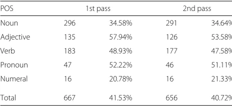
Finally, Table 13 shows the results for inflectional parts of speech, where the correct POS and the correct lemma but the false word form were recognized. These errors indicate falsely recognized word endings. The percentage values are given relative to the total number of tution errors of the POS, e.g., 866 nouns were substi-tuted with other nouns, while 296 of these substitutions (34.58%) were with a noun with the same lemma. We see that approximately 40% of all errors on inflectional parts of speech are due to falsely recognized word forms. In
Table 11Comparison of recognition errors by type between the first and second pass
Error type 1st pass 2nd pass Difference
Deletion 1446 1216 −230
Insertion 401 498 97
Substitution 4013 4043 30
Table 12Comparison of recognition errors by POS between the first and second pass
POS Total 1st pass 2nd pass Difference
Noun 6721 23.20% 23.26% +0.25%
Verb 3901 28.22% 27.66% −2.00%
Adjective 2646 20.67% 20.33% −1.65%
Adverb 1667 24.84% 24.18% −2.66%
Pronoun 1536 34.18% 33.27% −2.67%
Numeral 747 27.31% 27.71% +1.47%
Preposition 2499 27.53% 26.65% −3.19%
Conjunction 1964 28.16% 26.78% −4.88%
Particle 1038 24.76% 24.47% −1.17%
Interjection 8 100.00% 50.00% −50.00%
Residual 6 66.67% 100.00% +50.00%
the second pass, the total number of errors decreased by 1.65% relatively.
8 Conclusions
In the present paper, we proposed a new method of deter-mining the backoff path for factored language models. As the basic method leads to data sparsity and a large search space, we also presented all of the necessary algo-rithms to build a feasible system. We demonstrated that models using these backoff paths outperformed factored language models using more simply determined backoff paths. We also demonstrated that simpler models might not have any potential to improve recognition results, while the use of models with context-dependent back-off paths resulted in an accuracy improvement that was shown to be statistically significant.
The methods presented still leave room for the further optimization of several parameters used in the algorithms. Training set and factor selection may also be considered in further research. While we performed the experiments on Slovene, the proposed models can also be used in other inflectional or otherwise morphologically complex
Table 13Falsely recognized word forms of inflectional parts of speech relative to the total number of substitutions within the same part of speech
POS 1st pass 2nd pass
Noun 296 34.58% 291 34.64%
Adjective 135 57.94% 126 53.58%
Verb 183 48.93% 177 47.58%
Pronoun 47 52.22% 46 51.11%
Numeral 16 20.78% 16 21.33%
Total 667 41.53% 656 40.72%
languages. Further research on the possibility of com-bining the presented statistics-based method with formal knowledge-based methods could also lead to improve-ments in recognition of word relations in a spoken sen-tence and consequently to a reduction in recognition errors.
Acknowledgements
This work was partially financially supported by the Slovenian Research Agency (ARRS) under contract number 1000-10-310131.
Authors’ contributions
This paper shows results from the doctoral research of GD under the supervision of ZK. Both authors read and approved the final manuscript.
Competing interests
The authors declare that they have no competing interests.
Received: 13 October 2016 Accepted: 20 February 2017
References
1. S Zablotskiy, K Zablotskaya, W Minker, inIntelligent Environments (IE), 2010 Sixth International Conference on. Some approaches for Russian speech recognition, (Kuala Lumpur, 2010), pp. 96–99
2. T Rotovnik, MS Mauˇcec, Z Kaˇciˇc, Large vocabulary continuous speech recognition of an inflected language using stems and endings. Speech Commun.49(6), 437–452 (2007)
3. K Kirchhoff, D Vergyri, J Bilmes, K Duh, A Stolcke, Morphology-based language modeling for conversational Arabic speech recognition. Comput. Speech Lang.20(4), 589–608 (2006)
4. AE Axelrod,Factored language models for statistical machine translation. (University of Edinburgh, 2006)
5. EM de Novais, Portuguese text generation using factored language models. J. Brazilian Comput. Soc.19(2), 135–146 (2013)
6. K Kirchhoff, J Bilmes, K Duh,Factored language models tutorial. (University of Washington, 2016). http://ssli.ee.washington.edu/people/duh/papers/ flm-manual.pdf. Accessed 1 October
7. JA Bilmes, K Kirchhoff, inNAACL-Short ’03. Factored language models and generalized parallel backoff, (Edmonton, 2003), pp. 4–6
8. M Laz˘ar, D Militaru, inSpeech Technology and Human - Computer Dialogue (SpeD), 2013 7th Conference on. A Romanian language modeling using linguistic factors, (Cluj-Napoca, 2013), pp. 1–6
9. D Vazhenina, K Markov, inAwareness Science and Technology and Ubi-Media Computing (iCAST-UMEDIA), 2013 International Joint Conference on. Factored language modeling for Russian LVCSR, (Aizuwakamatsu, 2013), pp. 205-211
10. I Kipyatkova, A Karpov, inSPECOM 2014. Study of morphological factors of factored language models for Russian ASR, (Novi Sad, 2014), pp. 451–458
11. H Sak, M Saraçlar, T Güngör, inICASSP. Morphology-based and sub-word language modeling for Turkish speech recognition, (Dallas, 2010), pp. 5402–5405
12. MY Tachbelie, ST Abate, W Menzel, inLanguage and Technology Conference. Morpheme-based and factored language modeling for amharic speech recognition, (Pozna ˇn, 2011), pp. 82–93
13. Z Alumae, inICASSP. Sentence-adapted factored language model for transcribing estonian speech, (Toulouse, 2006), pp. 429–432 14. T Hirsimaki, J Pylkkonen, M Kurimo, Importance of High-Order N-Gram
Models in Morph-Based Speech Recognition. IEEE Trans. Audio, Speech, Lang. Process.17(4), 724–732 (2009)
15. AED Mousa, MAB Shaik, R Schlüter, H Ney, inINTERSPEECH. Morpheme based factored language models for German LVCSR, (Florence, 2011), pp. 1053–1056
16. H Adel, NT Vu, K Kirchhoff, D Telaar, T Schultz, Syntactic and Semantic Features For Code-Switching Factored Language Models. IEEE/ACM Trans. Audio, Speech, Lang. Process.23(3), 431–440 (2015)
18. T Erjavec, D Fišer, S Krek, N Ledinek, inLREC. The JOS Linguistically tagged corpus of Slovene, (Valletta, 2010), pp. 1806–1809
19. S Katz, Estimation of probabilities from sparse data for the language model component of a speech recognizer. IEEE Trans. Acoust. Speech, Signal Process.35(3), 400–401 (1987)
20. D Klakow, J Peters, Testing the correlation of word error rate and perplexity. Speech Commun.38(1–2), 19–28 (2002)
21. A Žgank, D Verdonik, AZ Markuš, Z Kaˇciˇc, inINTERSPEECH. BNSI Slovenian broadcast news database—speech and text corpus, (Lisbon, 2005), pp. 1537–1540
22. Š Arhar, V Gorjanc, S Krek, inProceedings of the Corpus Linguistics Conference. FidaPLUS corpus of Slovenian. The new generation of the Slovenian reference corpus: its design and tools, (Birmingham, 2007) 23. A Stolcke, J Wheng, W Wang, V Abrash, inProceedings IEEE Automatic
Speech Recognition and Understanding Workshop. SRILM at sixteen: update and outlook, (Waikoloa, 2011)
24. SF Chen, J Goodman, An empirical study of smoothing techniques for language modeling. Comput. Speech Lang.13(4), 359–394 (1999)
Submit your manuscript to a
journal and benefi t from:
7Convenient online submission 7Rigorous peer review
7Immediate publication on acceptance 7Open access: articles freely available online 7High visibility within the fi eld
7Retaining the copyright to your article