GENERALIZED FOURIER TRANSFORMS, INVERSE PROBLEMS, AND
INTEGRABILITY IN 4+2
A.S. Fokas
1Abstract. Three different types of generalized Fourier transforms are discussed, which appear in the following: (a) The medical imaging technique called Single Photon Emission Computerized Tomogra-phy (SPECT). (b) The solution of the Cauchy problem of integrable nonlinear evolution PDEs in 4+2, i.e. in four spatial and two temporal dimensions. (c) The characterization of the generalized Dirichlet to Neumann map for integrable nonlinear evolution PDEs in 1+1, i.e. in one spatial and one temporal dimensions.
1.
Introduction
Let the scalar valued function µ(x, y, k) satisfy the eigenvalue equation Lµ =f(x, y), where L is a linear differential operator in∂xand∂y depending onk∈C, where (x, y)∈R2. The spectral analysis of this equation
consists of the construction of two maps: In the construction of the direct map, the equationLµ=f is solved for µ in terms of f for all complex k. In the construction of the inverse map, µ is expressed in terms of an appropriate spectral function of f by formulating either aRiemann-Hilbert problem or a ¯∂ problem in the complexk-plane.
Suppose that the spectral function of f involves an integral transform of f. Then the above formalism provides a method for inverting this integral transform.
We recall that the classical derivation of transform pairs involves the integration in the complex k-plane of an appropriate Green’s function. However, this derivation is based on the assumption that the Green’s function is an analytic function ofkand it also assumes completeness. The assumption of analyticity corresponds to the case that µ is sectionally analytic. Therefore, the approach reviewed here has the advantage that, not only it provides a simpler approach to deriving classical transforms avoiding the problem of completeness, but also it can be applied to problems that the associated Green function isnot an analytical function ofk.
The above general formalism will be illustrated in section 2 for the particular case that the relevant integral transform is the attenuated Radon transform.
Let the scalar valued function µ(x1, x2, y1, y2, k) satisfy the eigenvalue equation Lµ = f(x1, x2, y1, y2)µ,
where Lis a linear differential operator in∂xj and ∂yj, j= 1,2, depending onk∈Cand (x1, x2, y1, y2)∈R4.
Proceeding as above and formulating anonlocal ∂¯-problem (instead of a Riemann-Hilbert or a ¯∂ problem), we can derive a nonlinear Fourier transform in four spatial dimensions. Such a transform is presented in section 3; this transform can be used for the solution of the Cauchy problem of a 4+2 generalization of the celebrated Kadomtsev-Petriashvilli equation. Reductions to 3+1 will also be mentioned.
The main difficulty with boundary value problems stems from the fact that only a subset of the boundary values is prescribed as boundary conditions. The determination of the unknown boundary values in terms of the
1 Department of Applied Mathematics and Theoretical Physics, University of Cambridge, Cambridge, CB3 0WA, UK
c
EDP Sciences, SMAI 2009
given boundary conditions is often called the Dirichlet to Neumann map. Although the terminology is usually used for elliptic problems, the question of determining the Dirichlet to Neumann map, or more precisely the generalized Dirichlet to Neumann map, is also important for evolution PDEs. For example, letq(x, t) satisfy
iqt+qxx= 0, 0< x <∞, 0< t < T, (1.1)
q(x,0) =q0(x), 0< x <∞, (1.2a)
q(0, t) =g0(t), 0< t < T, (1.2b)
whereq0(x) andg0(t) have appropriate smoothness,q0(x) has appropriate decay as|x| → ∞, andq0(0) =g0(0).
In this particular case determining the Dirichlet to Neumann map means expressingqx(0, t) in terms ofq0(x)
andg0(t). This problem can be solved by the classical Fourier transform inversion formula (after the change of
variablesk→k2). The analogous problem for the nonlinear Schrodinger equation is discussed in section 3.
2.
The Radon and Attenuated Radon Transforms
Let the lineLmake an angleθwith the positivex1-axis. A point (x1, x2) on this line can be specified by the
variables (τ, ρ), whereρis the distance from the origin and τ is a parameter along the line, see Figure 2.1.
τ
θ
(x , x ) 1 2
0 ρ
Figure 2.1
A unit vectorkalongLis given by (cosθ,sinθ), thus
(x1, x2) =τ(cosθ,sinθ) +ρ(−sinθ,cosθ).
Hence
x1=τcosθ−ρsinθ, ρ=x2cosθ−x1sinθ,
x2=τsinθ+ρcosθ, τ =x2sinθ+x1cosθ. (2.1)
The Radon transform of a functionf(x1, x2)∈S(R2), which will be noted by ˆf(ρ, θ), is defined as the integral
off alongL, i.e.,
ˆ
f(ρ, θ) =
Z ∞
−∞
f(τcosθ−ρsinθ, τsinθ+ρcosθ)dτ, ρ∈R, 0< θ < π. (2.2)
The attenuated Radon transform of a function g(x1, x2)∈ S(R2) with attenuationf(x1, x2) ∈ S(R2), which
will be denoted by ˆgf(ρ, θ),is defined by
ˆ
gf(ρ, θ) =
Z ∞
−∞
g(τcosθ−ρsinθ, τsinθ+ρcosθ)dτ, ρ∈R, 0< θ < π. (2.3)
The Radon transform can be inverted in a simple way using the Fourier transform. Also, it can be inverted via the spectral analysis of the following eigenvalue equation for the scalar function µ(x1, x2, k):
1 2(k+
1
k) ∂µ ∂x1
+ 1 2i(k−
1
k) ∂µ ∂x2
=f(x1, x2), −∞< x1, x2<∞, k∈C. (2.4)
Indeed, using this equation it was shown in [1] that
f(x1, x2) =− i
4π2(∂x1−i∂x2) Z 2π
0
eiθJ(x1, x2, θ)dθ, (2.5)
whereJ is the Hilbert transform with respect toρof ˆf(ρ, θ) evaluated atρ=x2cosθ−x1sinθ, i.e.,
J(x1, x2, θ) =
Z ∞
−∞
− fˆ(ρ
0, θ)dρ0
ρ0−(x
2cosθ−x1sinθ). (2.6)
It was shown by Novikov in [2] that the spectral analysis of the eigenvalue equation
1 2(k+
1
k) ∂µ ∂x1 +
1 2i(k−
1
k) ∂µ
∂x2 +f(x1, x2)µ=g(x1, x2), −∞< x1, x2<∞, k∈
C, (2.7)
yields the following formula for the inverse attenuated Radon transform: g(x1, x2) is given by the rhs of equation
(2.5), where nowJ is defined by
J(x1, x2, θ) =−e
R∞
τ f(scosθ−ρsinθ,ssinθ+ρcosθ)ds
eP−fˆ(ρ,θ)P−e−P−fˆ(ρ,θ)+e−P+fˆ(ρ,θ)P+eP+fˆ(ρ,θ)gˆ
f(ρ, θ);
(2.8) in this equation,ρand θ are given in terms ofx1 andx2 by the second set of equations (2.1) andP∓ denote
the usual projectors in the variableρ, i.e.
(P∓f)(ρ) =∓f2+ 1
2iπHf. (2.9)
It was shown in [3] that equation (2.7) can be reduced to equation (2.4), hence the inversion formula for the attenuated Radon transform is the direct consequence of the spectral analysis of the equation (2.4) performed in [1].
In order to construct the direct map associated with equation (2.4) we change variables from (x1, x2) to
(z,z¯), where
z= 1 2i(k−
1
k)x1−
1 2(k+
1
k)x2. (2.10)
Then equation (2.4) becomes
ν(k)∂µ
∂z¯ =f, ν(k) := 1 2i
1
|k|2 − |k|
2. (2.11)
We supplement equation (2.11) with the boundary condition
µ=O
1
z
, z→ ∞. (2.12)
µ(x1, x2, k) = 1
2πisgn
1
|k|2 − |k| 2
Z Z
R2 f(x0
1, x02)dx01dx02
z0−z , |k| 6= 1. (2.13)
This equation provides the direct map, i.e., it expresses µ in terms off(x1, x2). In order to construct the
inverse problem, i.e. in order to express µ in terms of an appropriate spectral function, we note thatµ is an analytic function ofkin the entire complexk-plane (including infinity) except for the unit circle. Thus in order to reconstructµ, it is sufficient to compute the “jump”µ+−µ−, whereµ+ andµ− denote the limits ofµas k
approaches the unit circle from inside and outside the unit disk. A simple computation yields [3]
µ±= lim
ε→0µ(x1, x2,(1∓ε)e
iθ) =∓P∓fˆ(ρ, θ)−Z ∞
τ
f ds, (2.14)
where P∓ denote the usual projectors in the variable ρ defined in equation (2.9) and H denotes the Hilbert
transform.
Equations (2.14) imply
µ+−µ−=−Hfˆ(ρ, θ)
iπ . (2.15)
Substituting this expression in the equation
µ= 1 2iπ
Z 2π
0
(µ+−µ−)(eiθ0)ieiθ0dθ0 eiθ0
−k , |k| 6= 1, (2.16)
we findµin terms of ˆf,
µ(x1, x2, k) =−
1 2iπ2
Z 2π
0
eiθ0
Hf dθˆ 0 eiθ0
−k . (2.17)
This equation provides the inverse map. Substituting this expression in equation (2.4) we find the inverse Radon transform formula (2.5) and (2.6).
We now present the derivation of the inverse attenuated Radon transform. Equation (2.7) can be rewritten in the form
ν(k)∂µ
∂¯z +f(x1, x2)µ=g(x1, x2), (2.18)
wheref ∈S(R2),g∈S(R2),k∈C, and |k| 6= 1. Equation (2.18) implies
µexp
∂−1
¯
z
f ν
=∂−1 ¯
z
g
ν exp
∂−1 ¯
z
f ν
. (2.19)
This equation provides the solution of the direct problem, i.e. it expresses µ in terms of f and g. Since µis an analytic function ofkin the entire complex k-plane except for the unit circle, it follows thatµ satisfies the alternative representation (2.16). Thus, in order to express µin terms of an appropriate spectral function, all that remains is to compute µ+−µ−. But this can be easily derived using equation (2.14). Indeed, equation
(2.11) can be rewritten in the form
lim
k→k±
∂−1
¯
z
f(x
1, x2)
ν(k)
=∓P∓fˆ(ρ, θ)− Z ∞
τ
f ds. (2.20)
Using this equation, equation (2.19) can be used to computeµ±, and then equation (2.16) provides an alternative
representation ofµin terms of ˆgf(ρ, θ) and off. Substituting this representation in equation (2.7) we find the
Remark 2.1. The Radon transform provides the mathematical foundation of Computerized Tomography as well as of Positron Emission Tomography, whereas the attenuated Radon transform provides the mathematical foun-dation of Single Photon Emission Computerized Tomography (SPECT) [4]. The latter technique has important applications in many areas of medicine including oncology, cardiology and neurology. The numerical imple-mentation of the inverse attenuated Radon transform using either cubic splines or Chebysev approximations is presented in [3] and [5]. A typical numerical implementation using the numerical technique of filter back projection is shown in the image (c) of Figure 2.2. Figures (b),(c),(d) depict the numerical reconstructions of the realistic cardiac phantom depicted in Figure (a), using three different models. The reconstruction (b) uses the approximation of zero attenuation which reduces the attenuated Radon transform to the classical Radon transform. The reconstruction in (d) uses an improved mathematical model for SPECT (which takes into ac-count the fact that the collimator actually receives ”cones” instead of rays); this leads to a modified attenuated Radon transform which can also be inverted analytically [6]. The incorporation of noise to these analytical algorithms is a difficult problem which is under consideration.
Figure 2.2: Different reconstructions of a cardiac phantom.
3.
A Nonlinear Fourier Transform in 4 Dimensions and the Generalized KP
Equation
Let
x=x1+ix2, y=y1+iy2, k=k1+ik2, λ=λ1+iλ2,
where x1, x2, y1, y2, k1, k2, λ1, λ2 are real variables. We will use the shorthand notation F(x, y, k, λ) for the
function F(x1, x2, y1, y2, k1, k2, λ1, λ2).
Letµ(x, y, k) satisfy the scalar eigenvalue equation
µy¯−µ¯x¯x−2kµx¯+f(x, y)µ= 0.
By performing the spectral analysis of this equation and by employing a non-local ¯∂ formulation the following nonlinear Fourier transform (FT) of f is constructed in [7]:
Direct nonlinear FT:R4→R4:f(x1, x2, y1, y2)→fˆ(k1, k2, λ1, λ2)
ˆ
f(k, λ) = 2
π3
Z
R4
(¯λ−k¯) ¯E(k, λ, x, y)f(x, y)µ(x, y, λ)dxdy, (3.1a)
whereE denotes the exponential
E(k, λ, x, y) =e2i[(λ2−k2)x1+(k1−λ1)x2+2(λ1λ2−k1k2)y1+(k21−k 2 2+λ
2 2−λ
andµis uniquely defined in terms off by the following integral equation:
µ(x, y, k) = 1 +
Z
R4
G(x−x0, y−y0, k)f(x0, y0)µ(x0, y0, k)dx0dy0, (3.2a)
where the function Gis defined by
G(x, y, k) =−π14
Z
R4
eξx−ξ¯x¯+ηy−η¯y¯
−η¯−ξ¯2+ 2kξ¯dξdη, ξ=ξ1+iξ2, η=η1+iη2.
Inverse nonlinear FT:R4→R4: ˆf(k1, k2, λ1, λ2)→f(x1, x2, y1, y2)
f(x, y) = 2
π∂¯x Z
R4
E(k, λ, x, y) ˆf(k, λ)µ(x, y, λ)dkdλ, (3.1b)
whereµis uniquely defined in terms of ˆf by the linear integral equation
µ(x, y, k) = 1 + 1
π Z
R4
E(k0, λ, x, y) ˆf(k0, λ)µ(x, y, λ)dk0dλ
k−k0, k∈C. (3.2b)
If appropriate norms of f and ˆf are sufficiently small thenµ can be approximated by 1 and equations (3.1) reduce to the classical FT pair in four dimensions [7].
It was shown in [7] that the nolinear FT pair (3.1) can be used to solve the Cauchy problem for the following equation in the variableq(x, y, t):
q¯t=
1 4q¯x¯xx¯−
3 2qqx¯+
3 4∂
−1 ¯
x qy¯y¯, ∂x−¯1f
(x) = 1
π Z Z
R2
f(x)dx0 1dx02
x−x0 , (3.3)
t=t1+it2,(t1, t2)∈R2, q(x, y,0) =q0(x, y).
Equation (3.3) is an integrable generalisation of the KP equation in 4+2 dimensions, i.e. four spatial (x1, x2, y1, y2)
and two temporal (t1, t2) dimensions.
The following reductions of the potential version of equation (3.3) are also integrable [8]:
qt1 =
1
4qx1x1x1−
3 8(q
2
x1−q
2
x2) +
3 4∂
−1
x1qy1y1, ∆q= 0, (3.4)
qt2 =−
1
4qx2x2x2−
3
4qx1qx2−
3 4∂
−1
x2qy1y1, ∆q= 0, (3.5)
where
∆ =∂2
x1+∂
2
x2. (3.6)
4.
The Dirichlet to Neumann Map for the NLS
Equation (1.1) is equivalent to the statement that the following differential form is closed:
W =eikx+ik2t[qdx+ (iqx+kq)dt], 0< x <∞,0< t < T, k∈C. (4.1)
Assuming thatq(x, t) has sufficient decay asx→ ∞for all 0< t <∞, and employing Green’s theorem, equation (4.1) implies the following global relation:
ˆ
q0(k)−i
Z T
0
eik2sq
x(0, s)ds+k
Z T
0
eik2sq(0, s)ds=eik2Tqˆ
where ˆq0(k) and ˆqT(k) denote the Fourier transform ofq0(x) and q(x, T). The first and the third terms of the
lhs of equation (4.2) are known, but the term ˆqT(k) involves the unknown functionq(x, T). Actually, causality
implies thatqx(0, t) cannot depend on the “future time”T, hence the term ˆqT(k)cannotcontribute toqx(0, t).
This motivates the following approach for solving equation (4.2) for qx(0, t): The classical Fourier transform
inversion formula (after the change of variablesk2→l) indicates that in order to invert the integral appearing
in the lhs of equation (4.2) we must multiply this integral with kexp[−ik2t]. The function ˆq
T(k) is analytic
for Imk >0 and the function exp[ik2(T−t)] is bounded and analytic for k in the union of the first and third
quadrants of the complex k-plane. Hence, the product kexp[ik2(T −t)]ˆq
T(k) is bounded and analytic in the
first quadrant of the complexk-plane and is ofO(1) ask→ ∞. Thus, by integrating around the boundary of the first quadrant denoted by ∂I and by appealing to Jordan’s lemma (after the change of variablesk2 →l),
it follows that the integral of the above product vanishes. Hence, equation (4.2) yields the following expression forg1(t) =qx(0, t):
g1(t) =
Z
∂I
ke−ik2t "
Z ∞
0
eikxq0(x)dx−k
Z T
0
eik2sg0(s)ds
#
dk, 0< t < T. (4.3)
By changing the order of thex−ands−integrations with thek-integration and then by computing thek-integrals (see [9] for details), we find that equation (4.3) simplifies to the following equation
g1(t) =−
1
√ πe
−iπ
4
1
√ t
Z ∞
0
eix 2
4t q˙0(x)dx+
Z t
0
˙
g0(s)
√ t−sds
, 0< t < T. (4.4)
The occurrence of the derivatives ˙q0and ˙g0is due to the fact that in order to obtain well defined k-integrals we
first integrate by parts thex−ands−integralsbefore changing the order of integration. Letq(x, t) satisfy the following initial-boundary value problem:
iqt+qxx−2|q|2q= 0, 0< x <∞,0< t < T
q(x,0) = 0, 0< x <∞, (4.5)
q(0, t) =g0(t), 0< t < T,
whereg0(t) has sufficient smoothness andg0(0) = 0. Our goal is to determineg1(t) =qx(0, t) in terms ofg0(t).
In this case the analogue of the global relation (4.1) is the following equation [9]
Z T
0
e2ik2
τ
i|g0(τ)|2Φ1(τ, k)−[2kg0(τ) +ig1(τ)]Φ2(τ, k) dτ =e4ik
2
Tc+(k), Imk
≥0, (4.6)
where c+(k) is an analytic function ofk for Imk >0 and of order O(1/k) ask → ∞. The functions Φ 1 and
Φ2 are certain solutions of the t-dependant part of the associated Lax pair. The integral involving g1(τ), in
addition to the exponential exp[2ik2τ], it also contains the function Φ 2(τ, k).
This function makes thek-dependence prohibitively complicated for the application of the Fourier inversion formula. This observation motivates the following question. Does there exist a representation of (Φ1,Φ2)
in-volving exponential dependence on k? The answer is positive and such a formula is provided by the so called Gelfand-Levitan-Marchenko (GLM) representation [10]: The vector Φ can be represented in the form
Φ(t, k) =
0
eif2t
+
Z t
−t
L1(t, s)−2ig0(t)M2(t, s) +kM1(t, s)
L2(t, s) +iρ2g¯0(t)M1(t, s) +kM2(t, s)
eif2sds, (4.7)
where the functions{Lj, Mj, Nj}21 satisfy the following equations:
L1(t, t) =
i
L1t−L1s=ig1(t)L2+α(t)M1+β(t)M2,
L2t+L2s=−iρ¯g1(t)L1−α(t)M2+ρβ¯(t)M1,
M1t−M1s = 2g0(t)L2+ig1(t)M2,
M2t+M2s = 2ρ¯g0(t)L1−iρ¯g1(t)M1,
(4.9)
withα(t) andβ(t) defined by the equations
α(t) =ρ
2(g0g¯1−g¯0g1), β(t) = 1
2(ig˙0−ρ|g0|
2g
0). (4.10)
Using the GLM representation we will now show that the Neumann boundary valuesg1(t) =qx(0, t) can be
expressed in terms of the Dirichlet boundary valueg0(t) by the following formula [11],[12]:
g1(t) =g0(t)M2(t, t)−e −iπ
4 √
π Z t
0
∂M1
∂τ (t,2τ −t) dτ √
t−τ. (4.11)
Indeed, replacing the function Φ1 by the rhs of (4.7) in the global relation (4.6) we find
Z t
0
e4ik2
τ
L1(t,2τ −t)−
i
2g0(t)M2(t,2τ−t) +kM1(t,2τ −t)
dτ
=−e
4ik2
t
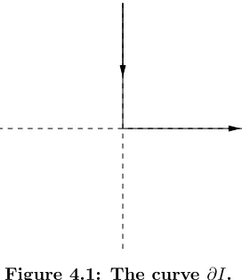
2 C(k, t), Imk≥0, 0< t < T. (4.12) We multiply this equation by kexp[−4ik2t0], t0 < t, and integrate along the boundary of the first quadrant of
the complexk-plane, which we denote by∂I, with the orientation shown in Figure 4.1.
Figure 4.1: The curve ∂I.
The rhs of the resulting equation vanishes because kc+(k, t) is analytic and of O(1) for Imk >0, and the
oscillatory term exp[ik2(t−t0)] is bounded in the first quadrant.
The first two terms of the lhs of equation (4.12) give contributions which can be computed in closed form using the following identity
Z
∂I
k Z t
0
e4ik2
(τ−t0)K(τ, t)dτ
dk= π
4K(t
0, t), t >0, t0 >0, t0< t (4.13)
terms of the lhs of equation (4.12) yield
π
4
L1(t,2t0−t)−
i
2g0(t)M2(t,2t
0 −t)
. (4.14)
Before computing the contribution of the third term in the lhs of equation (4.12), we first use integration by parts:
Z t
0
ke4ik2
τM
1(t,2τ−t)dτ =
1 4ik
h e4ik2
tM
1(t, t)−M1(t,−t)
i
−41ik Z t
0
e4ik2
τ∂M1
∂τ (t,2τ−t)dτ. (4.15)
Multiplying this term bykexp[−4ik2t0] and integrating along∂I, we find three contributions. The first vanishes
due to the fact that exp[4ik2(t−t0)] is bounded in the first quadrant of the complexk-plane. Thek-integral of
the second contribution can be computed in closed form: usingk2t0=l2 we find
Z
∂I
e−4ik2t0dk=
Z
∂I
e−4il2√dl t0 =
c √
t0,
with
c=
Z
∂I
e−4il2 dl=1
2
Z
∂I
e−il2 dl= 1
2
Z ∞
−∞ e−il2
dl=
Z ∞
0
e−il2 dl=1
2e −iπ 4 Γ 1 2
, (4.16)
where in deforming∂I to the real axis we have used the fact that exp(−il2) is bounded in the second quadrant
of the complexk-plane.
In order to compute the contribution of the third term in the rhs of equation (4.15) we splitRt
0 into
Rt0
0 and
Rt
t0. The contribution of the second integral vanishes due to analyticity considerations and the contribution of
the first integral yields ak-integral which equalsc/√t0−t. Thus, equation (4.12) yields
π
4
L1(t,2t0−t)− i
2g0(t)M2(t,2t
0−t)
−4ci "
M1(t,−t)
√ t0 +
Z t0
0
∂M1
∂τ (t,2τ−t) dτ √
t0−τ #
= 0.
Letting t0→t, the above equation becomes equation (4.11).
References
(1) A.S. Fokas and R. G. Novikov, Discrete Analogues of the Dbar Equation and of Radon Transform, C.R. Acad. Sci., Paris313,75-80 (1991).
(2) R. G. Novikov, An Inversion Formula for the Attenuated X-ray Trasnformation, Ark. Mat. 40, 145 (2002).
(3) A.S. Fokas, A. Iserles and V. Marinakis, Reconstruction Algorithm for Single Photon Emission Com-puted Tomography and its Numerical Implementation, J. R. Soc. Interface 3, 45 (2006).
(4) M.N. Wernick and J.N. Aarsvold, Eds.,Emission Tomography, The Fundamentals of PET and SPECT, Elsevier Academic Press, USA (2004).
(5) A.S. Fokas and V. Marinakis, Reconstruction Algorithm for the Brain Imaging Techniques of PET and SPECT, Hermis Intern. Journal 4, 45-61 (2004).
(7) A.S. Fokas, The D-Bar Method, Inversion of Certain Integrals and Integrability in 4 + 2 and 3 + 1 Dimensions, J. Phys. A, 41, 344006 (2008).
(8) A.S. Fokas, Soliton Multidimensional Equations and Integrable Evolutions Preserving Laplace’s Equa-tion, Phys. Lett. A372, 1277-1279 (2008).
(9) A.S. Fokas,A Unified Approach to Boundary Value Problems, CBMS-NSF Regional Conference Series in Applied Mathematics78, SIAM, USA (2008).
(10) A. Boutet de Monvel and V. Kotlyarov, Scattering Problem for the Zakharov-Shabat Equations on the Semi-Axis, Inverse Problems16, 1813-1837 (2000).
(11) A. Boutet de Monvel, A.S. Fokas and D. Shepelsky, The Analysis of the Global Relation for the Nonlinear Schr¨odinger Equation on the Half-Line, Lett. Math. Phys. 65, 199-212 (2003).