University of Mazandaran, Iran http://cjms.journals.umz.ac.ir ISSN: 1735-0611 CJMS.3(2)(2014), 227-232
B-Spline Finite Element Method for Solving Linear System of Second-Order Boundary Value Problems
A. Yazdani1and S. Gharbavi 2
Department of Mathematics, University of Mazandaran, Babolsar, Iran.
Abstract. In this paper, we solve a linear system of second-order boundary value problems by using the quadratic B-spline finite el-ement method (FEM). The performance of the method is tested on one model problem. Comparisons are made with both the analyti-cal solution and some recent results.The obtained numerianalyti-cal results show that the method is efficient.
Keywords: Finite element method; Quadratic B-splines ; Bound-ary Value Problems.
2000 Mathematics subject classification: 34B05; Secondary 80M10.
1. Introduction
System of ordinary differential equations have been applied to many problems in physics, engineering, biology and so on. There are many publications dealing with the linear system of second-order boundary value problems. For instance, B-spline method has been proposed in [4]. Spline functions are a class of piecewise polynomials which satisfy continuity properties depending on the degree of the polynomials. They have highly desirable characteristics which have made them a powerful mathematical tool for numerical approximations. Spline functions are a set of continuous combinations of B-splines that used as trial functions in the Galerkin methods [5, 7, 12, 13, 14]. The finite element method was
1Corresponding author: [email protected] Received: 25 November 2013
Revised: 23 February 2014 Accepted: 24 February 2014
introduced and analyzed for semilinear parabolic problems by Zlamal in [16]. Later Xiong and Chen [15] studied superconvergency of triangular quadratic finite element for semilinear elliptic problem and illustrated the effectiveness of the proposed method.
The quadratic B-splines incorporated with finite element methods have been proven to give very smooth solutions[1, 2, 3, 8, 9, 10, 11, 6], and the use of the quadratic B-splines as shape functions in the finite ele-ment method guarantees continuity of the first and second-order deriva-tives of trial solutions at the mesh points.
In this paper, we present and analyze the B-spline finite element method for solution of a linear system of second-order boundary value problems. The paper is organized as follows: in section 2, the proper-ties of the quadratic B-spline finite element are discussed, the numerical experiments and data comparisons are provided to verify the accuracy and efficiency. The last section is conclusion.
2. Analysis of B-spline finite element method
We consider the following linear system of second-order boundary value problem:
u00+a1(x)u0+a2(x)u+a3(x)v00+a4(x)v0+a5(x)v=f1(x),
v00+b1(x)v0+b2(x)v+b3(x)u00+b4(x)u0+b5(x)u=f2(x),
u(0) =u(1) = 0, v(0) =v(1) = 0,
(2.1)
where ai(x),bi(x),f1(x) and f2(x) are given functions, and ai(x), bi(x) are continuous, i= 1,2,3,4,5.
DefineH01(I), I = (0,1) by
H01(I) =
w|w∈H1(I), , w(0) =w(1) = 0 . (2.2)
The variational problem accordance with (2.1) is: Find u, v∈H1 0(0,1)
such that
−hu0, w0i+ha1u0, wi+ha2u, wi − ha3v0, w0i+ha4v0, wi+ha5v, wi
=hf1, wi,
−hv0, w0i+hb1v0, wi+hb2v, wi − hb3u0, w0i+hb4u0, wi+ha5u, wi
=hf2, wi,
(2.3)
for all w∈H01(0,1),wherehu, wi=R01uwdx.
required properties are defined by
φm= 1 h2
(xm+2−x)2−3(xm+1−x)2+ 3(xm−x), [xm−1, xm],
(xm+2−x)2−3(xm+1−x)2, [xm, xm+1],
(xm+2−x)2 [xm+1, xm+2],
0 otherwise.
(2.4) whereh=xm+1−xm,m=−1,0,· · ·, N. The quadratic B-splineφm(x) and its first derivative vanishes outside the interval [xm−1, xm+2]. The
value of φm and its first derivativeφ0(x) at the knots are given by:
x xm−1 xm xm+1 xm+2
φm(x) 0 1 1 0
φ0m(x) 0 2/h −2/h 0
Let
uN(x) = N X
j=−1
Cjφj(x), vN(x) = N X
j=−1
Djφj(x), (2.5)
be an approximate solution of (2.1), where Cj and Dj are unknown real coefficients which must be determined. Each B-spline covers three intervals so that three B-splinesφm−1, φm, φm+1cover each finite element
[xm, xm+1]. All other B-splines are zero in this region.
Using Eq. (2.4), the nodal valueum, vm, u0m and v0m at the knot xm can be expressed in the terms of the coefficientsCj and Dj as
um :=uN(xm) =Cm−1+Cm, vm :=vN(xm) =Dm−1+Dm,
u0m :=u0N(xm) = 2
h(Cm−Cm−1), v
0
m :=vN0 (xm) = 2
h(Dm−Dm−1). (2.6)
Since uN(x) and vN(x) must satisfy the boundary conditions uN(0) =
uN(1) = 0 and vN(0) =vN(1) = 0, we get C−1 = −C0, CN =−CN−1,
D−1 =D0 and DN =DN−1. Hence, we have
uN(x) = N−1
X
j=0
Cjψj(x), vN(x) = N−1
X
j=0
whereψ0=φ0(x)−φ−1(x) , ψm=φm, m= 1,2,· · ·, N −2 and
ψN−1=φN−1−φN(x). Hence 2N unknownsCm, Dm ,m= 0,1, · · ·, N −1 must be determined.
According to Galerkin method, the weight functionw(x) in Eqs.(2.3) is chosen as w(x) =ψn(x), n= 0,1,· · · , N −1.
Putting Eqs.(2.7) in Eqs.(2.3), we have a system of linear equations. This system can be written in the matrix-vector form as follows:
RX=F, (2.8)
where
X=
C0, C1,· · · , CN−1, D0, D1,· · · , DN−1 T
,
F =
Z 1
0
f1ψ0dx,· · ·, Z 1
0
f1ψN−1dx, Z 1
0
f2ψ0dx,· · · , Z 1
0
f2ψN−1dx T
,
R=
M1 | M2
−− −− −−
M3 | M4
2N×2N
,
and four tridiagonal submatricesM1, M2, M3, M4 as follows:
(M1)ij =− Z 1
0
ψj0ψ0idx+
Z 1
0
a1(x)ψj0ψidx+ Z 1
0
a2(x)ψjψidx
(M2)ij =− Z 1
0
a3(x)ψj0ψi0dx+ Z 1
0
a4(x)ψj0ψidx+ Z 1
0
a5(x)ψjψidx
(M3)ij =− Z 1
0
ψj0ψ0idx+
Z 1
0
b1(x)ψ0jψidx+ Z 1
0
b2(x)ψjψidx
(M4)ij =− Z 1
0
b3(x)ψ0jψ 0 idx+
Z 1
0
b4(x)ψ0jψidx+ Z 1
0
b5(x)ψjψidx
where i= 0,· · ·, N −1, j= 0,· · · , N−1.
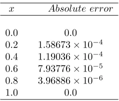
Example 2.1. Consider the following system of second-order boundary value problem
u00(x) +xu(x) +xv(x) =f1(x),
v00(x) + 2xv(x) + 2xu(x) =f2(x),
subject to boundary conditionsu(0) =u(1) = 0,v(0) =v(1) = 0 where 0< x <1,f1(x) = 2 andf2(x) =−2. The exact solutionu(x),v(x) are
Table 1. The maximum absolute error for Example 2.1
whenh= 411.
x Absolute error
0.0 0.0 0.2 1.58673×10⁻⁴
0.4 1.19036×10⁻⁴
0.6 7.93776×10⁻⁵
0.8 3.96886×10⁻⁶
1.0 0.0
Figure 1. Result for Example 2.1 with u(x) =x2−xand
v(x) =x−x2.
3. Conclusion
In this paper, B-spline finite element method using quadratic B-spline basis functions has been successfully used to develop the solution of lin-ear system of second-order boundary value problems. We have seen that the numerical technique presented here is capable enough of producing numerical solution of high accuracy. The B-spline FEM is very benefi-cial for getting the numerical solutions of the differential equations when continuity is the basic requirement. Given technique is flexible enough and can be applied to other complex problems which are difficult to solve directly.
References
[1] E. N. Aksan, Quadratic B-spline finite element method for numerical solu-tion of the Burgers equasolu-tion,Applied Mathematics and Computation,174
(2006) 884-896.
[2] A. R. Bahadir, Application of cubic B-spline finite element technique to the thermistor problem, Applied Mathematics and Computation, 149 (2004) 379-387.
[3] N. Caglar, H. Caglar, B-spline solution of singular boundary value prob-lems,Applied Mathematics and Computation,182(2006) 1509-1513.
[4] N. Caglar, H. Cagler, B-spline method for solving linear system of second-order boundary value problems,Computers and Mathematics with Applications, 57(2009) 757-762.
[5] S. Dhawan, S. Kapoor, S. Kumar, Numerical method for advection diffu-sion equation using FEM and B-splines,Journal of Computational Science,
3(2012) 429-437.
[7] L. R. T. Gardner, G. A. Gardner, I. Dag, A B-spline finite element method for the regularized long wave equation,Commum. Numer. Meth. Eng., 11
(1995) 59-68.
[8] D. Idris, M. Naci Ozer, Approximation of the RLW equation by the least square cubic B-spline finite element method, Applied Mathematical Mod-elling,25 (2001) 221-231.
[9] S. Kutluay, A. Esen, A B-spline finite element method for the thermistor problem with the modified electrical conductivity, Applied Mathematics and Computation, 156(2004) 621-632.
[10] S. Kutluay, A. Esen, I. Dag, Numerical solutions of the Burgers equation by the least-squares quadratic B-spline finite element method,Computational and Applied Mathematics, 167(2004) 21-33.
[11] Q. Lin, Y. Hong Wua, R. Loxton, S. Lai, Linear B-spline finite element method for the improved Boussinesq equation, Journal of Computational and Applied Mathematics, 224(2009) 658-667.
[12] T. Ozis, A. Esen, S. Kutluay, Numerical solution of Burgers equation by quadratic B-spline finite elements,Applied Mathematics and Computation,
165(2005) 237-249.
[13] L. Ronglin, N. Guangzheng, Y. Jihui, B-spline finite element method in polar coordinates,Finite Elements in Analysis and Design,28(1998) 337-346.
[14] D. Sharma, R. Jiwari, S. Kumar, Numerical Solution of Two Point Bound-ary Value Problems Using Galerkin-Finite Element Method,International Journal of Nonlinear Science,13(2012) 204-210.
[15] Z. G. Xiong, C. M. Chen, Superconvergence of triangular quadratic finite element method with interpolated coefficients for nonlinear elliptic prob-lem, Acta Math. Sci.,26(2006) 174-182 .
[16] M. Zlamal, A finite element solution of the nonlinear heat equation,