Simplified approach to DFT computation for nonprogrammable scientific calculators

R C

O S T N

Publisher: Research Council of Science and Technology, Biratnagar, Nepal p. 13

BIBECHANA

A Multidisciplinary Journal of Science, Technology and Mathematics ISSN 2091-0762 (print), 2382-5340 (online)

Journal homepage: http://nepjol.info/index.php/BIBECHANA

Simplified approach to DFT computation for nonprogrammable

scientific calculators

Mohd Yusuf Yasin

ECE Department, Integral University, Kursi Road, Lucknow, Uttar Pradesh, India, PIN 226026, Email: [email protected]

Accepted for publication: December 6, 2014

Abstract

Fourier analysis is an important tool used as it is or it’s different variants in many fields of sciences and engineering. It’s importance is due to it’s simplicity with which it expands a given function in terms of circular or complex exponents. Further it is quite versatile to handle many functions of practical interest, specifically, the functions with several mathematical disabilities that are hard to be handled with tools like Taylor series. Discrete Fourier Transform (DFT) is a form of Fourier analysis where the discrete function and it’s transform are both of finite length. This processing requires lot many computations. Here in this work a simplified and non programmable calculator based scheme is presented with which one can easily determine the DFT of the given function by feeding in the DFT equation once and a few presses of the calculator keys.

DOI: http://dx.doi.org/10.3126/bibechana.v12i0.11681 © 2014 RCOST: All rights reserved.

Keywords: Fourier analysis; DFT computation; scientific calculator.

1. Introduction

Engineering is so heavily endowed with the mathematics that it may be hard to find out a single topic of mathematics that is never used in any application; engineering and mathematics run side by side and are naturally inseparable from one another. More sophisticated engineering applications usually involve advanced mathematics. Engineering point of view is to achieve the solution with a certain tolerances. This is a necessary design parameter that involves a compromise between the efforts required to obtain the final solution and the total time spent in achieving it. Bode’s plotting is a popular example, where error at a corner frequency is substantially high (3dB maximum), accuracy of the function is sacrificed at the corner, but it pays off by enhancing the speed in estimating the characteristics of a system containing several distinguished poles and zeros, of different types, in just a few steps [1]. Optimization of speed and efforts seem to occupy the central place in design and analysis. However, the accuracy is all important and may not be sacrificed every time.

Yasin./ BIBECHANA 12 (2015) 13-19: p. 14

cumbersome computational procedures, which unfortunately leads to the failure in maintaining interest in computation [2]. Here in this work, the discrete Fourier Transform

(DFT) computation is presented, which normally demands a good some of mathematical calculations, usually involving complex numbers. Computation with complex numbers is as easy a task as the computation with real numbers [3], and hence the DFT of a function can also be easily computed.

2. Fourier Analysis

Fourier analysis expands a periodic function in terms of the sum of simple circular functions. It finds applications in engineering systems analysis, mathematical analysis, mechanics, audio and video signal processing. It is considered more versatile than Taylor series, as it can expand many discontinuous functions of practical interest [4]. Different versions of Fourier analysis practically exist, for periodic and non periodic functions, which may be continuous or discrete. Fourier series is used for periodic functions whereas Fourier transforms are used for aperiodic functions.

It is of particular importance that when a discrete function of finite sample length is analyzed, the corresponding Fourier transform is also discrete. Such a function has both the Fourier series and Fourier transforms similar [5].

Let {x[n]}be an aperiodic finite energy sequence of sample length N, x[n] being a discrete function, ‘n’ being integer and is uniformly spaced in time. Actually the independent variable n being ‘nT’, T is the time period of sampling function, though T is dropped for the sake of simplicity. A periodic representation of the function x[n] is defined by

∑ −

= ∞ −∞ =

l

p n x n lN

x ( ) ( ) (1)

Fourier series representation of (1) over N samples can be given by the following synthesis – analysis pair.

∑ ≤ ≤ −

= −

=

− 1

0

2

1 0

) ( 1 N

n

nk N j

p

k x n e k N

N c

π

(2)

∑ −∞< <∞ = −

= 1

0 2 )

( N

k

nk N j k

p n c e n

x

π

(3)

Similarly the Fourier transform pair for the finite sequence {x(n)} can be given by.

∑ ≤ ≤ −

= − =

− 1

0

2

1 0

) ( )

( N

n

nk N j

N k e

n x k X

π

(4)

∑ ≤ ≤ −

= −

= 1

0

2

1 0

) ( 1 )

( N

k

nk N j

N n e

k X N n x

π

(5)

Yasin./ BIBECHANA 12 (2015) 13-19: p. 15

k

Nc k

X( )= (6)

This type of analysis requires a set of cumbersome computations as it involves complex numbers. The

equations (2 – 5) are in fact N equations each one containing N terms with a weight _e jNnk

π

2 ±

But in practical computations, a little manipulation can lead to simpler computations for the above analysis, which can be run on a simple non-programmable calculator. Here it is demonstrated through an example, how this can be accomplished with affordable simple equation(s). 6 point analysis of an arbitrary sequence x(n) = {2, 1, -3, 4} can be performed by using Equation (4).

∑ = ∑ = = − − = − 5 0 3 1 0 2 ) ( ) ( ) ( n nk j N n nk N j e n x e n x k X π π (7) 5 , 4 , 3 , 2 , 1 , 0 ; 4 3 1 2 )

(_k = + _e− 3 − _e− 32 + _e− 33 _k =

X j k j k j k

π π

π

(8)

The exponent of (7), could be expressed in calculator syntax.

(

)

nk nk nk j nk j e

e 1 60

3 1 3

3 _ = ∠−

     _∠− =         = − − π π

π

(9)

(

1 60

)

1

3 = ∠− =

−j nk _nk

e

π

(10)

(

1∠−60

)

m =

(

1∠−60m

)

(11)

Using equations (9) and (11), equation (8) can be rewritten as

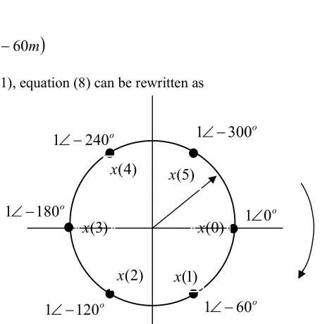
Fig. 1: Points of DFT computation uniformly placed on the unit circle, alongwith the points of data of the function x(n) mapped to the circle.

(

)

(

)

( )

k k

k k

X k k k

180 1 * 4 120 1 * 3 60 1 * 1 2 1 4 120 1 3 60 1 1 2 ) ( − ∠ + − ∠ − − ∠ + = − + − ∠ − − ∠ + = ₍₁₂₎ o

60

1

∠

−

o

240

1

∠

−

o

180

1

∠

−

o 120 1∠−

o

300

1

∠

−

o

0

1

∠

)

0

(

x

)

1

(

x

) 2 ( x

)

3

(

x

)

4

(

Yasin./ BIBECHANA 12 (2015) 13-19: p. 16

Equation (12) can be implemented directly on a calculator, k replaced by a memory, say A, and with modes be set CMPLX and DEG. Once the equation (12) is fed, the press of the key CALC asks for the value of “A” and offers the corresponding DFT component at a consecutive press of the = key. The result is presented below.

{

4, 1.732,7 3.464, 6,7 3.464, 1.732

}

)

(k j j j j

X = − − + − (13)

The process to approach equation (12) is still simple and can also be written by considering the fact that the computation points are uniformly distributed over the circle of unit radius by a phase 2π_N radians in the 2

π

phase space. With the help of Figure 1, DFT equation can be written directly.

k k

k

x x

x k

X( )= (0)(1∠0) + (1)(1∠−60) +...+ (5)(1∠−300) ₍₁₄₎

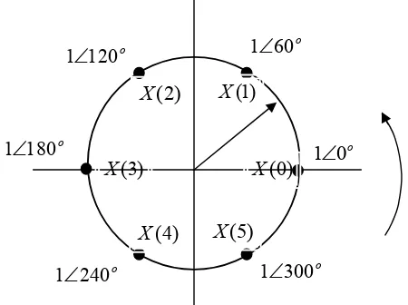
Similarly, the inverse DFT (IDFT) computation is also as simple, and can again be directly written with the help of Figure 2, keeping in mind that the weights in the IDFT Equation as follows.

Fig. 2: IDFT computation scheme. IDFT computation points uniformly placed on the unit circle, alongwith the DFT mapped on the circle.

(

n n n

)

X X

X N n

x( )= 1 (0)(1∠0) + (1)(1∠60) +...+ (5)(1∠300) ₍₁₅₎

Perhaps, the equations (14) and (15) are in their simplest possible form. Other forms are also possible

involving conjugate weights, as the weights corresponding to ∠₆₀

is conjugate to ∠₃₀₀

and vice versa, and may be incorporated if needed. Generalized equations based on the representations of equations (14) and (15) can thus be given as follows.

(

)

k

N

n N

n n

x k

X = ∑− ∠− =

1

0

2 1 ) ( )

( π (16)

o 300 1∠ o

120 1∠

o 180 1∠

o 240 1∠

o 60 1∠

o

0

1

∠

) 0 ( X

)

5

(

X

) 4 ( X ) 3 ( X

)

2

(

Yasin./ BIBECHANA 12 (2015) 13-19: p. 17

(

)

n

N

k N

k k X N n

x = ∑− ∠ =

1

0

360 1 ) ( 1 )

(

(17)

3. DFT Computation – Schemes and Results

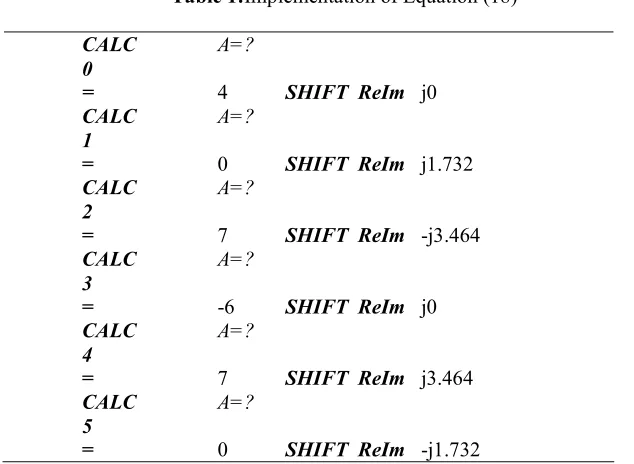
The procedure of DFT computation on CASIO calculators like fx 991ES PLUS Natural V.P.A./M., can be summarized as follows. Use of equation (12) or (14) can facilitates to write an equation in calculator syntax for the discrete sequence x(n)={2, 1, -3, 4}. The computation is done in a bit interactive manner as presented in Table 1 below. In Bold and Italic, are the calculator key presses required right from the basic equation and the components of the results are in normal text.

A

A

A

₃

₁₂₀

₄

₁₈₀

60

1

2

+

∠

−

−

∠

−

+

∠

−

(18)

Table 1:Implementation of Equation (18)

CALC A=?

0

= 4 SHIFT ReIm j0

CALC A=?

1

= 0 SHIFT ReIm j1.732

CALC A=?

2

= 7 SHIFT ReIm -j3.464

CALC A=?

3

= -6 SHIFT ReIm j0

CALC A=?

4

= 7 SHIFT ReIm j3.464

CALC A=?

5

= 0 SHIFT ReIm -j1.732

Hence the result is

X

(

k

)

=

{

4

,

j

1

.

732

,

7

−

j

3

.

464

,

−

6

,

7

+

j

3

.

464

,

−

j

1

.

732

}

. Similarly the IDFT computation can also be done through a similar procedure. Thus

(

₄

+

j

₁₇₃₂

_*

₁

∠

₆₀

A

+

₍

₇

−

j

₃

_.

₄₆₄

₎

₁

∠

₁₂₀

A

−

₆₁

∠

₁₈₀

A

+

6

1

)

A

j

A

j

₃

_.

₄₆₄

₎

₁

₂₄₀

₁

_.

₇₃₂₁

₃₀₀

7

(

+

∠

−

∠

(19)

Yasin./ BIBECHANA 12 (2015) 13-19: p. 18

powers higher than 3. For example, in Casio fx-991W S-V.P.A.M., one can adopt another simple yet

elegant method. Let _{a e} jN

π

2 −

= , Equation (4) can be rearranged as follows.

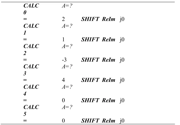
Table 2:Implementation of Equation (19)

CALC A=?

0

= 2 SHIFT ReIm j0

CALC A=?

1

= 1 SHIFT ReIm j0

CALC A=?

2

= -3 SHIFT ReIm j0

CALC A=?

3

= 4 SHIFT ReIm j0

CALC A=?

4

= 0 SHIFT ReIm j0

CALC A=?

5

= 0 SHIFT ReIm j0

))))

1

(

)

2

(

(

...

)

3

(

(

)

2

(

(

)

1

(

(

)

0

(

)

(

k

=

x

+

a

x

+

a

x

+

a

x

+

a

x

n

−

+

a

x

n

−

X

k k k k k (20)

Use of Equation (20) can facilitate to overcome the complex power limitation of a calculator. Considering the use of calculator memories A and B, and the CMPLX mode, a simple algorithm can be suggested as follows.

B A N j N

e−jN =_cos(2 ₎− _sin(2 ₎→ → 2

π

π

π

{

)))) 1 ( ) 2 ( ( ... ) 3 ( ( ) 2 ( ( ) 1 ( ( ) 0 ( )

(k =x +A x +A x +A x + A x k− +Ax k − X

B A A= *

) (k X CALC

Repeat if k ≤N−1.

} (21)

Yasin./ BIBECHANA 12 (2015) 13-19: p. 19

Initialize e−j = − j )=0.62349− j0.78183→A→B

7 2 sin( ) 7 2 cos(

7

2π _{π π}

.

Feed

1

+

A

(

2

+

A

(

3

+

4

A

))

= X(1)= -2.0245 - j6.2240

RCL A RCL B = AB=−0.22252− j0.974928→A. Display

1

+

A

(

2

+

A

(

3

+

4

A

))

, = X(2) = 0.3460 + j2.4791

Display AB→A = -0.9010 - j0.4339

Display1+ A(2+A(3+4A)), = X(3)= 0.1784 -j2.4220.

Repeat this and obtain X(4)= 0.1784 + j2.4220, X(5)= 0.3460 - j2.4791, and X(6)= -2.0245 + j6.2240. The method is so simple that the DFT computation is merely a matter of a minute. IDFT

computation is similar except the initialization of memories for _e jN

π

2 +

and each X(k) must be divided by N.

Unfortunately, stacking in CMPLX mode is limited to level 2 only. Moreover, the power of complex

number is up to only 3, the built-in function. The power may be resolved like

A

5

=

A

3

.

A

2. Combining the stacking and power resolving, the range for DFT/IDFT computation can be easily raised.

4. Conclusion

The scheme presented above can be applied to real or complex functions both, with the same ease. Radix – 2 algorithms popular for DFT/IDFT computation, but these algorithms also get more and more complicated for Radix >3. However, the scheme presented here is simple and is Radix independent and can be considered as a tool as far as the textual length of the equations (16) or (17) is permissible by a calculator display. For educational purpose, usually small order computations are considered, therefore, the scheme presented here can be a useful method.

References

[1] J. Millman, A. Grabel, Microelectronics, 2nd Edition, 25th reprint, India edition,Tata McGrawHill. (2010).

[2] M. Y. Yasin, BIBECHANA 8 (2012) 31-36. http://dx.doi.org/10.3126/bibechana.v8i0.4702 [3] M. Y. Yasin, BIBECHANA 9 (2013) 18-27.

http://dx.doi.org/10.3126/bibechana.v9i0.7148

[4] E. Kreyszig, Advanced Engineering Mathematics, 5th edition, John Wiley & Sons. Inc., 5th Wiley eastern reprint (1989).