Contributing Authors
Alexander Antonov
Ilja Faerman
Michael Konikov
Dan Li
Serguei Mechkov
Ion Mihai
Vladimir Pavlov
Michael Spector
Ping Sun
Leonard Tchuindjo
Review Committee
Dawn Patrick
Serguei Issakov
Alexander Antonov
Satyam Kancharla
Jim Jockle
Editorial Committee
Nic Trainor
Anna Basanskaya
Journal Designer
Joanna Wilkiewicz
Managing Editor
Hong Wang
Numerix Journal
Wednesday 27th May, 2015
Copyright c⃝2015 by Numerix LLC All rights reserved.
Complying with all applicable copyright laws is the responsibility of the user. Without limiting its rights under copyright, no part of this document may be reproduced, stored in or introduced into a retrieval system or transmitted in any form or by any means (electronic, mechanical, photocopying, recording, or otherwise), or for any purpose, without the express written permission of Numerix LLC.
The Free-Boundary SABR: Natural Extension to Negative Rates . . . 4
Martingale and Distribution Tests for the Libor Market Model . . . 15
“Hot-Start” Initialization of the Heston Model . . . 22
Featured Articles on Numerix Products and Services
Negative Rates: The Challenge and the Opportunity. . . 29
The Free Boundary SABR: Natural Extension to Negative Rates
Alexandre Antonov* Michael Konikov† Michael Spector‡
Abstract
In the current low-interest-rate environment, extending option models to negative rates has become an important issue. This paper describes one such extension of the widely used SABR model. We stress that our solution is more natural and attractive than the shifted SABR model. An exact formula is derived for option prices in the case of zero correlation between the rate and its volatility. For nonzero correlation, a mapping procedure onto a mimicking zero-correlation model is applied. Analytical results from the suggested free-boundary SABR model are compared with Monte Carlo simulation results.
1 Introduction
The SABR process with parameters(F0, v0, β, ρ, γ)1 [7] for a rateFtand its volatilityvt has the SDE
dFt=FtβvtdW1, (1.1)
dvt=γ vtdW2, (1.2)
with correlationE[dW2dW1] =ρdtand power 0 ≤β <1. The solution is not uniquely defined by the SDE—we also need to impose boundary conditions. The standard choice is to assume that the boundary at zero is absorbing, which enforces positivity and martingality of the rate. See [2], [4], [6], [8], [9], [10], [13] for further references.
The SABR model is primarily used for volatility cube interpolation and for pricing CMS products by replication with vanilla options. It is also used in term-structure models, e.g., [12], [14].
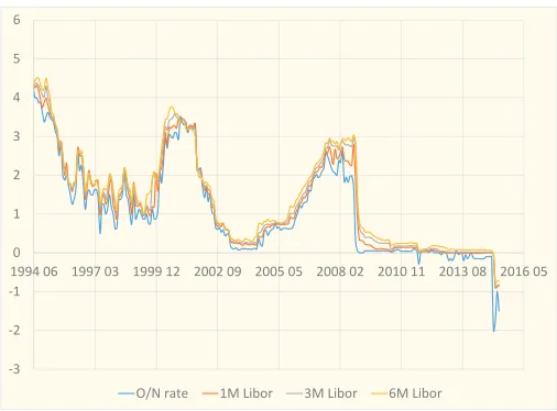
When the SABR model was first introduced, rate positivity seemed like a reasonable and attractive property. In the current market environment, where rates are extremely low and sometimes even neg-ative, it is important to extend the SABR model to negative rates. For example, Figure 1 shows the historical evolution of Swiss Franc (CHF) interest rates. One observation is that rates reached as low as −2%. Another important observation is that the rates “stick” to zero for certain periods of time, suggesting that their probability density functions have a singularity at zero.
The simplest way to take negative rates into account is to shift the SABR process
dFt= (Ft+s)βvtdW1,
where sis a deterministic positive shift. This moves the lower bound ofFtfrom0 to−s.
One can either include the shift in the calibration parameters(v0, β, ρ, γ,s)or fix it prior to calibration (e.g., to2% in the case of Swiss Franc short rates). Each alternative has drawbacks.
Ͳ3
Ͳ2
Ͳ1 0 1 2 3 4 5 6
199406 199703 199912 200209 200505 200802 201011 201308 201605
[image:5.612.180.433.91.278.2]O/Nrate 1MLibor 3MLibor 6MLibor
Figure 1: Swiss Franc interest rates.
If we fix the shift from the very beginning and calibrate the standard parameters(v0, β, ρ, γ), there are still drawbacks. There is always the danger that rates can go lower than anticipated, in which case we would need to change this parameter accordingly. This can result in a jump in the other SABR parameters as a calibration response to such readjustment. As a consequence, we can get jumps in the values/Greeks of the trades dependent on swaption or cap volatilities. To cover for potential losses in such situations, traders are likely to be asked to reserve part of their P&L. Also, having the swaption prices bounded from above (due to the rate being bounded from below) can lead to situations when the shifted SABR model cannot attain market prices. In sum, we need a more natural and elegant solution for permitting negative rates.
Forβ= 0, the normal SABR model,dFt=vtdW1, allows the rates to become negative when a free boundary condition is enforced. Below, we come up with a generalization of this model
dFt=|Ft|βvtdW1
with0≤β < 12 and afreeboundary. As we will see, such a model allows for rates that can be negative and exhibit a certain “stickiness” at zero.
In what follows, we consider only theF0>0case (unless explicitly stated otherwise). WhenF0<0, we note thatFt˜ =−Ftsatisfies the SABR SDE with parameters(−F0, v0, β,−ρ, γ), and the time value
of a European option onFtstruck at Kequals that of an option on Ft˜ struck at −K.
To get intuition about the free boundary, we start with a CEV exampledFt=|Ft|βdWand study the PDF and option prices. Then we switch to the SABR model with a free boundary condition and present an exact solution for the zero-correlation case. For the general case, we show an accurate approximation for European options prices. We demonstrate that the exact formula as well as its approximation can be presented in terms of a 1D integral over elementary functions, making it well-suited for fast calibration.2
We finish with simulation schemes and numerical results.
2
CEV Process
To aid with intuition, we consider the CEV model dFt = FtβdW with 0 ≤ β < 1. The forward
Kolmogorov (FK) equation on the density p(t, f),
pt−1
2 (
f2βp)f f = 0,
has two types of solutions, depending on the boundary conditions; fixing the PDE (or SDE) alone is not sufficient to uniquely define the solution. One can show (e.g., [5]) that there are two distinct solutions with asymptotics pA∼f1−2β andpR∼f−2β. We call the first solution absorbing and the second one reflecting. The latter exists only forβ < 12; otherwise, the norm around zero diverges.
The asymptotics are closely related to conservation laws, which can be obtained by integrating the FK equation by parts against some payoffs h(f). Consider first the norm case h(f) = 1. It is easy to see the asymptotic behavior of the absorbing solution leads to nonconservation of the norm, while the reflecting solution conserves the norm. For the first moment conservation, we take h(f) = f and deduce that the asymptotics of the reflecting solution leads to nonconservation of the first moment (i.e., nonmartingality), while the absorbing solution is a martingale.
The explicit PDFs for the CEV process are known (see [11] and [5]) in terms of the modified Bessel functions, which permits us to calculate a call option time-value via the time integral without the boundary term:
O(T, K) =E[(FT −K)+]−(F0−K)+= 1 2K
2β ∫ T
0
dt p(t, K). (2.1)
As explained in [5], this is not the case for put options, where a boundary term is present.
Below we will need option prices for absorbing/reflecting solutions as 1D integrals (see [3] and [5]). These are given by
OA/R(T, K) =
√ KF0
π
(∫ π
0
sin(|ν|θ)sin(θ)
b−cos(θ) e
−q¯(b−cos(θ))
T dθ
+sin(|ν|π) ∫ ∞
0
e∓|ν|xsinh(x) b+cosh(x) e
−q¯(b+cosh(x))
T dx )
(2.2)
for an indexν =−2(11−β) and parameters
¯
q=q0qK, b= q2
0+qK2
2q0qK , q0= F01−β
1−β and q= K1−β
1−β.
Now consider an extension of the CEV model to the entire real line by modifying the SDE to
dFt=|Ft|βdW (2.3)
for0≤β < 12. The corresponding FK equation is
∂tp(t, f) = 1 2 (
|f|2βp(t, f))f f. (2.4)
Anorm conservingandmartingale solution that satisfies the FK equation with the initial condition
p(0, f) =δ(f−F0)can be constructed from the reflecting and absorbing solutions as
p(t, f) = 1
2(pR(t,|f|) +sign(f)pA(t,|f|)). (2.5)
We can get the same expression for the density with a purely probabilistic argument. For anyf >0, a reflecting path ending at f is equivalent to a free-boundary path ending atf or −f, and vice versa. For the absorbing case, we apply the reflection principal as usual, which involves taking the probability of a path ending atf and subtracting the probability of the path ending atf and touching zero, which is equivalent to a path ending at −f. Hence, we can write the linear system
Ͳ0.25
Ͳ0.15
Ͳ0.05 0.05 0.15 0.25 0.35 0.45 0.55
Ͳ10 Ͳ5 0 5 10
P
D
F
[image:7.612.211.403.94.233.2]strikeinforwardunits
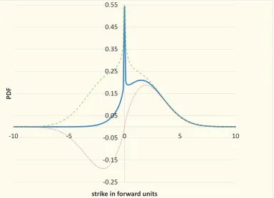
Figure 2: The blue solid line represents the free PDF, the red dotted line depicts the absorbing density expression sign(f)pA(t,|f|), while the green dashed line gives
the symmetrical reflecting solution.
Note that the PDF diverges as p(t, f) ∼ |f|−2β at zero. (The asymptote is inherited from the
reflecting solution.) The observed singularity is quite natural: one can observe a “sticky” behavior of real rates near zero in, for example, the behavior of the CHF rate in Figure 1.
A call option payoffh(f) = (f −K)+ leads to an option time value of
OF(T, K) = 1 2|K|
2β ∫ T
0
dt p(t, K) =1 2|K|
2β ∫ T
0 dt1
2(pR(t,|K|) +sign(K)pA(t,|K|))
= 1
2(OR(T,|K|) +sign(K)OA(T,|K|)). (2.6)
Finally, we present the free CEV option integral. Its time value can easily be derived from the absorbing-reflecting solutions (2.2) and (2.6), yielding
OF(τ, K) = √
|KF0| π
( 1K≥0
∫ π
0
sin(|ν|θ)sinθ b−cosθ e
−q¯(b−cosθ)
τ dθ
+sin(|ν|π) ∫ ∞
0
(1K≥0cosh(|ν|x) +1K<0sinh(|ν|x))sinhx
b+coshx e
−q¯(b+coshx)
τ dx )
, (2.7)
where ν=−2(11−β) and
¯
q=|F0K|
1−β
(1−β)2 with b=
|F0|2(1−β)+|K|2(1−β)
2|F0K|1−β .
We will use this formula to derive the analytics for the SABR model in the section below. Note that we put the absolute value ofF0 for symmetry with respect to the strike: F0 is assumed to be positive, consistent with the remark in the introduction.
Regarding the sensitive region of small strikes and/or small rates, we see that the call option price (the full one, including the intrinsic value) is a smooth function ofK andF0at zero. Thorough analysis reveals that the main terms of the expansion near zero are linear with the following terms of the order
|K|2(1−β)for small strikes and|F0|2(1−β)
for small spots.
3
SABR
Now, let us come back to the SABR process (1.1)–(1.2). The standard choice of the absorbing boundary will be generalized to afree boundary. Namely, we will consider the SDE
for 0 ≤β < 12 (with the same process (1.2) for the stochastic volatility). Such a construction permits both negativerates and “stickiness” at zero.
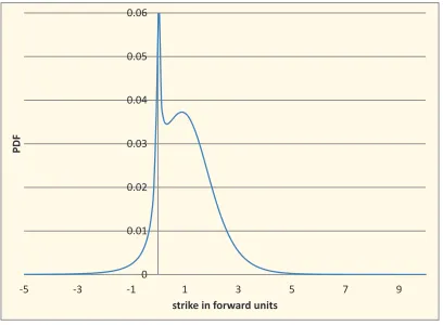
Looking forward, we plot the SABR density function, which is shown in Figure 3 for the Input I parameters from Table 4. We also observe the singularity at 0, which reflects the “sticky” behavior of rates at zero. (See Figure 1.)
0 0.01 0.02 0.03 0.04 0.05 0.06
-5 -3 -1 1 3 5 7 9
P
D
F
[image:8.612.205.409.166.316.2]strike in forward units
Figure 3: SABR model PDF forT = 3Y,β= 0.25.
3.1 Zero-Correlation Case
The zero-correlation free SABR model can be solved exactly. Indeed, the option price can be computed as
OSABR
F (T, K) =E [
OCEV
F (τT, K) ]
, (3.1)
whereOCEV
F (τ, K)is the free-boundary CEV option price (2.7), and the stochastic timeτT = ∫T
0 v 2 tdtis
the cumulative variance for the geometric Brownian motionvt(1.2). The dependence onτ in both inte-grand terms of (2.7) is of the form exp(−λ/τ). Thus, averaging over stochastic time,E[OCEV
F (τT, K) ]
,
requires calculating the mean value E[exp(−λ/τT)].
The moment generating function (MGF) of the inverse stochastic time was derived in [3] and given by E [ exp ( −λ τT )]
= G(T γ
2, s)
coshs for s=sinh
−1 (√
2λ γ v0
) .
The function
G(t, s) = 2√2 e
−t
8
t√2πt ∫ ∞
s
du u e−u
2 2t
√
coshu−coshs
has been introduced in [4]; it is closely related to the McKean heat kernel on the hyperbolic planeH2. It is important to notice that, although the function G(t, s) is a 1D integral, it can bevery efficiently approximated by a closed formula (see [4]).
Thus, the exact option price for the zero correlation case can be presented as
OSABR
F (T, K) =
1
π √
|KF0| {1K≥0A1+sin(|ν|π)A2}
with the integrals
Here shas the following parameterization with respect toϕandψ:
sinhs(ϕ) =γ v0−1√2¯q(b−cosϕ),
sinhs(ψ) =γ v0−1√2¯q(b+coshψ),
where q¯andbare the same as in the CEV free-boundary option.
3.2 General Correlation Case
As in [4], we approximate the general correlation option price by using the zero-correlation model
dFt˜ =|F˜| ˜ β
t ˜vtdW1,˜ d˜vt= ˜γvt˜ dW2,˜
with E[dW1˜ dW2˜ ] = 0. That is, we aim to find model parameters forF˜ so that
E[(Ft−K)+]≃E [
( ˜Ft−K)+ ]
.
For the freeboundary, we reuse the same effective coefficients of the zero-correlation SABR model as in [4] for theabsorbing boundary. The power and vol-of-vol are strike-independent with
˜
β =β and ˜γ2=γ2−3
2 {
γ2ρ2+v0γρ(1−β)F0β−1 }
,
while the initial stochastic volatility is more complicated and strike-dependent. The ˜v0 parameters can be calculated as an expansion
˜
v0= ˜v0(0)+T˜v(1)0 +· · ·. (3.4)
The leading volatility term can be expressed as
˜
v0(0)= 2 Φδq˜γ˜
Φ2−1 for Φ = (
vmin+ρv0+γ δq
(1 +ρ)v0 )˜γ
γ
, (3.5)
where
v2min=γ2δq2+ 2γρδqv0+v20, δq=
k1−β−F1−β 0
1−β and δq˜=
k1−β˜−F1−β˜ 0
1−β˜ . (3.6)
The effective strikek is afloored initial strike: all the effective parameters formulae based on the heat-kernel expansion work only for positive strikes. In our experiments, we used k=max(K,0.1F0). Note that the initial value of the rate F0 is considered to be positive. See the remark in the introduction for negativeF0.
The first-order correction is more complicated and is given by
˜
v0(1)
˜
v0(0)
= ˜γ2 √
1 + ˜R2 1 2ln
( v0vmin
˜ v(0)0 v˜min
) − Bmin
˜
Rln(√1 + ˜R2+ ˜R)
for R˜= δq˜γ ˜
v(0)0 ,
where ˜vmin= √
˜
γ2δq2+(v˜(0) 0
)2
andBminis the so-called parallel transport, defined as
Bmin=−12
β
1−β ρ √
1−ρ2 (
π−arccos
(
−δq γ+v0ρ vmin
)
and
I=
2 √
1−L2
(
arctan√u0+L
1−L2 −arctan
L √
1−L2
)
forL <1,
1 √
L2−1ln
u0(L+
√ L2−1)+1
u0(L−
√
L2−1)+1 forL >1,
(3.7)
where
L= vmin(1−β)
k1−βγ√1−ρ2 and u0=
δq γρ+v0−vmin
δq γ√1−ρ2 .
See also [9] and [13].
At the end of this section, we comment on the arbitrage-free property of the free-boundary SABR model. As arealprocess, the free-boundary SABR model is naturally arbitrage-free. On the other hand, its approximation described in this subsection is, strictly speaking, not arbitrage-free (except in the case of the zero correlation when the approximation becomes exact). However, in our efficient volatility expansion˜v0 we use thefixed efficient strikek= 0.1F0forK <0.1F0. This means that prices for such strikes are given by the zero-correlation model with strike-independent coefficients and, consequently, are arbitrage-free. For the other strikes, given high approximation accuracy, we can call the resulting analytical formulaquasi-arbitrage-free.
4 Numerical Experiments
Calibration to real data. We start with a real data example of a 1Y15Y CHF swaption from 10-Feb-2015 with a forward rate of F0 = 0.56%. The swaption prices are quoted in terms of normal
implied volatility (bps). We calibrate free-boundary and shifted SABR models to this data by using our analytical approximations. The output is presented in Table1 and graphed in Figure4.
Strike Target free-bdry shifted
0.06% 23.5 23.5 24.6
0.31% 44.7 44.5 43.3
0.56% 59.3 59.2 58.7
0.81% 71.7 71.7 71.8
1.06% 83.0 83.1 82.9
1.56% 103.5 103.8 103.6
[image:10.612.85.437.96.207.2]2.56% 140.4 140.2 140.7
0 20 40 60 80 100 120 140 160
0.06% 0.31% 0.56% 0.81% 1.06% 1.56% 2.56%
N
o
rm
a
l
v
o
l
(b
p
s)
Strike
CHF10ͲFebͲ151Y15Yvols
[image:11.612.204.410.93.242.2]Target freeͲbdry shifted
Figure 4: Plot of the free-boundary normal implied volatilities (bps) from Table1.
The calibration errors for the free-boundary SABR model and the shifted SABR model are shown in Figure 5. We see that the calibration error for the free-boundary SABR is small. Table2 shows the calibrated values ofα=v0,ρ, γ, andβ. The value of the shift for the shifted SABR model is2%.
Ͳ1.5
Ͳ1.0
Ͳ0.5 0.0 0.5 1.0 1.5
0.06% 0.31% 0.56% 0.81% 1.06% 1.56% 2.56%
E
rr
o
r
(b
p
s)
Strike CHF10ͲFebͲ151Y15Yerrors
[image:11.612.207.407.326.472.2]freeͲbdry shifted
Figure 5: Calibration errors (in bps) for free-boundary and shifted SABR models. Wee see that the free-boundary SABR model has less calibration error.
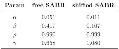
Param free SABR shifted SABR
α 0.051 0.011
β 0.417 0.167
ρ 0.990 0.999
γ 0.658 1.080
Table 2: Calibrated parameters for the free-boundary SABR and shifted SABR models.
Note the extremely high values of the correlation ρand fairly high values of the vol-of-vol γ. The reason for such high correlation is a very steep skew prevailing in the current CHF.
We now study theaccuracy of the analytical approximation for the free SABR model. First, let us briefly address the Monte Carlo simulation scheme. (See [5] for more details.) Suppose that we have simulated the stochastic volatility for all timesteps and paths vt.3 Our goal is to simulateFt+∆t given
[image:11.612.208.404.531.613.2]this information. The first thing to try is an Euler scheme without any boundary condition (i.e., a free boundary), which is
Ft+∆t=Ft+|Ft|βvt∆W1(t).
One can explicitly check that the Euler scheme does not work for points close to zero even when∆t→0. Instead, we need to come up with a more careful scheme based on a numerical inversion of the CDF, which can be found in [5]. However, such a procedure is very slow, and we prefer to come up with a regime-switching scheme similar to [1] in order to accelerate the simulations. For values away from the boundary, we use moment matching to approximate Ft+∆t via the quadratic Gaussian step, while for near-boundary values, we numerically invert the CDF.
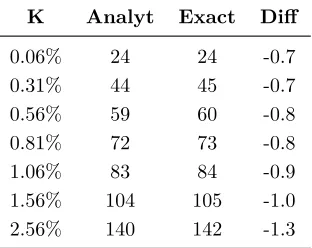
In Table 3, we compare the Monte Carlo simulations described above (Exact) and our analytical formula based on the map to the zero correlation SABR model (Analyt) for the calibrated parameters in Table2. As shown, the approximation is excellent.
K Analyt Exact Diff
0.06% 24 24 -0.7
0.31% 44 45 -0.7
0.56% 59 60 -0.8
0.81% 72 73 -0.8
1.06% 83 84 -0.9
1.56% 104 105 -1.0
[image:12.612.229.385.260.384.2]2.56% 140 142 -1.3
Table 3: Comparison of implied volatilities from Monte Carlo simulations (Exact) and the analytical formula (Analyt) with the parameters from Table2.
Approximation accuracy analysis. We analyze the approximation accuracy for two additional sets of inputs. These input data sets are negatively correlated, which is a more classical situation. The input data that is used is shown in Table4, and the implied volatilities from the Monte Carlo simulation method are compared against the analytical approximation for both sets of inputs in Table5.
Parameter Symbol Value for Input I Value for Input II
Rate Initial Value F0 50 bps 1%
SV Initial Value v0 0.6F
1−β
0 0.3F
1−β 0
Vol-of-Vol γ 0.3 0.3
Correlations ρ −0.3 −0.3
Skews β 0.25 0.25
Maturities T 3Y 10Y
[image:12.612.136.480.496.606.2]Input I Input II K Analyt Exact Diff Analyt Exact Diff
-0.95 30.87 30.93 -0.06 40.05 40.86 -0.81 -0.8 29.83 29.95 -0.12 38.43 39.24 -0.81 -0.65 28.80 28.97 -0.17 36.80 37.60 -0.80 -0.5 27.79 27.99 -0.20 35.18 35.97 -0.78 -0.35 26.83 27.04 -0.21 33.59 34.33 -0.74 -0.2 25.95 26.15 -0.20 32.05 32.73 -0.68 -0.05 25.30 25.46 -0.16 30.67 31.25 -0.58 0.1 25.77 25.85 -0.08 30.20 30.63 -0.43 0.25 26.63 26.69 -0.06 30.19 30.51 -0.31 0.4 27.33 27.39 -0.06 30.14 30.41 -0.27 0.55 27.90 27.97 -0.06 30.06 30.31 -0.25 0.7 28.38 28.45 -0.07 30.00 30.22 -0.23 0.85 28.80 28.87 -0.07 29.98 30.18 -0.20
1 29.18 29.25 -0.07 30.05 30.22 -0.17
[image:13.612.173.438.99.396.2]1.15 29.53 29.60 -0.07 30.24 30.36 -0.12 1.3 29.87 29.94 -0.07 30.56 30.63 -0.07 1.45 30.22 30.29 -0.06 31.03 31.04 -0.01 1.6 30.58 30.63 -0.06 31.63 31.58 0.04 1.75 30.95 30.99 -0.05 32.35 32.26 0.09 1.9 31.33 31.37 -0.04 33.17 33.04 0.13
Table 5: Differences in implied volatilities (in bps) between simulations (Exact) and an-alytics (Analyt). The bold line (K= 1) represents the ATM strike.
The implied volatility results that are shown in Table5 are plotted in Figure6
24.00 26.00 28.00 30.00 32.00 34.00 36.00 38.00 40.00
Ͳ1 Ͳ0.5 0 0.5 1 1.5 2
no
rm
a
l
v
o
l
(b
p
s)
strikeinforwardunits
Analyt,InputI Exact,InputI Analyt,InputII Exact,InputII
Figure 6: Plot of implied volatility for Monte Carlo simulation (Exact) and our method (Analyt).
[image:13.612.206.409.469.614.2]5
Conclusion
We presented a natural generalization of the SABR model to negative rates, which is very important in the current low-rate environment, and described its properties. We derived an exact formula for the option price in the zero-correlation case and an efficient approximation for the general correlation case written in terms of a one-dimensional integral of elementary functions. The simplicity of the approxi-mation allows for straightforward implementation. Moreover, the main formulae from our “absorbing” (standard) SABR approximation can be directly reused. Finally, we have numerically checked the accuracy of the approximation for option pricing.
Acknowledgments
The authors are indebted to Serguei Mechkov for discussions and help with the numerical implementation as well as to their other colleagues at Numerix, especially to Gregory Whitten and Serguei Issakov for supporting this work and to Nic Trainor for the excellent editing.
References
[1] Andersen, L. B. Efficient simulation of the heston stochastic volatility model. Available at http://ssrn.com/abstract=946405, 2007. Accessed 2014-10-03.
[2] Andreasen, J., and Huge, B. Expanded forward volatility. Risk Magazine(January 2013). [3] Antonov, A., Konikov, M., Rufino, D., and Spector, M. Exact solution to CEV model
with uncorrelated stochastic volatility, 2014. Available at SSRN.
[4] Antonov, A., Konikov, M., and Spector, M.SABR spreads its wings.Risk Magazine(August 2013), 58–63.
[5] Antonov, A., Konikov, M., and Spector, M. The free boundary SABR: Natural extension to negative rates. Available athttp://ssrn.com/abstract=2557046, 2015. Accessed 2015-02-27. [6] Balland, P., and Tran, Q. SABR goes normal. Risk Magazine(May 2013).
[7] Hagan, P. S., Kumar, D., Lesniewski, A. S., and Woodward, D. E. Managing smile risk.
Wilmott Magazine 1(November 2002), 84–108.
[8] Hagan, P. S., Kumar, D., Lesniewski, A. S., and Woodward, D. E. Arbitrage free SABR.
Wilmott Magazine(January 2014).
[9] Henry-Labordere, P. Analysis, Geometry, and Modeling in Finance: Advanced Methods in Option Pricing. Chapman & Hall, 2008.
[10] Islah, O. Solving SABR in exact form and unifying it with LIBOR market model. Available at http://papers.ssrn.com/sol3/papers.cfm?abstract_id=1489428009, 2009.
[11] Jeanblanc, M., Yor, M., and Chesney, M. Mathematical Methods for Financial Markets. Springer, 2009.
[12] Mercurio, F. Pricing inflation-indexed derivatives. Quantitative Finance (2005), 289–302. [13] Paulot, L.Asymptotic implied volatility at the second order with application to the SABR model.
Available athttp://ssrn.com/abstract=1413649, 2009.
Martingale and Distribution Tests for the Libor Market Model
Alexander Antonov* Dan Li† Leonard Tchuindjo‡
Abstract
Using martingale normalization, we find appropriate adjustment factors to simulated Libor rates, which we use for two purposes. First, we show that the adjusted model-simulated forward Libor rate is a martingale under the simulation measure. This allows us to construct a martingale restriction test for the Libor market model, which requires that in an arbitrage-free market, the expectation of each adjusted forward Libor rate simulated by a model calibrated to option-embedded instruments equals the corresponding forward Libor rate implied from the yield curve. This has practical implications for arbitrage trading. Second, we use the adjustment factors to construct a distribution test for the simulated forward Libor rates. We show how, in the simulated measure, the adjustment factors transform the distribution of each simulated Libor rate to match the initial distribution assumption of its corresponding forward Libor rate in its relevant measure. This has practical implications for model testing.
1
Introduction
The Libor market model (LMM) framework was independently proposed by Brace, Gatarek and Musiela [2] and Sandmann and Sonderman [13] and further improved by Jamshidian [9]. This framework is attractive because it can directly model observable rates such as Libor or swap rates, which is a significant improvement over short-rate models (e.g., Hull and White [8]) and forward-rate models (e.g., Heath, Jarrow, and Morton [10]), which model unobservable instantaneous rates.
The setup of the standard LMM is straightforward. We assume that each forward Libor rate follows a stochastic process with a known distribution under its relevant measure. However, because all rates are simultaneously simulated under a single measure, the stochastic differential equation (SDE) of each rate must be reformulated in this measure, which adds a time-dependent drift.1 As a result, each forward
Libor rate follows a stochastic process with a distribution that can be unknown in the simulating measure (especially if the initial process is lognormal). Market practitioners therefore face the problem of recovering the model distribution for the simulated forward Libor rate. For example, if the model setup assumes that each forward Libor is lognormal in its relevant measure, then one has to find a way to adjust the distribution of each simulated forward Libor so that it becomes lognormally distributed in the simulation measure. Constructing this adjustment allows us to test whether the distribution of the simulated forward Libor rates is concordant with the initial distribution assumption of the Libor market model.
Finding appropriate adjustments for the simulated forward Libor rate can also help verify the mar-tingale restriction for the Libor rate market. This means that in the absence of arbitrage, the forward Libor rate simulated by the LMM calibrated to option-embedded market instruments (such as caps, floors, and swaptions) equals the corresponding forward rate implied from the yield curve constructed from Libor-based instruments (such as cash Libor rates, forward rate agreements, Eurodollar futures,
*Numerix, SVP of Quantitative Research, [email protected]
†Numerix, SVP of Financial Engineering, [email protected]
‡Numerix, Director of Financial Engineering, [email protected]
1If the simulation is conducted in a measure associated with a particular rate, then the SDE for that rate under the
and swaps). The martingale restriction test can be conducted by using any option-pricing model to test for the absence of arbitrage in the corresponding market. Early studies were done by Longstaff [11], who conducted a test to check whether the underlying S&P value implied from call options on the S&P 100 through the model equals its actual market value. In [3], Brenner and Eom conducted the test on call and put options on the S&P 500. Busch [4] has also tested the martingale restriction on the USD-GBP call and put currency market. These authors conducted their analysis in the Black-Scholes framework. However, no such test has been done for Libor rates to the best of our knowledge.
We use martingale normalization to find appropriate adjustment factors, which are built upon a proposed sample stochastic discount factor, and show that when the simulated forward Libor rate is adjusted by these factors, its expectation under the simulating measure equals the value of the corre-sponding forward Libor rate implied from the yield curve. We set up a one-factor lognormal LMM and we check this condition with USD market data for 31 December 2014. We find that the adjusted forward three-month Libor rates simulated by the LMM calibrated to swaptions are very close to the forward three-month Libor rates implied from the Eurodollar futures and swap data. This shows that there are very limited arbitrage opportunities and negligible frictions in the USD Libor market.2 Furthermore,
we use the above factors to adjust the distributions of the simulated forward Libor rates so that they become lognormal. We thus recover the initial lognormal assumption of our LMM setup. A Kolmogorov-Smirnov test supports this finding. However, it is important to note that our proposed martingale and distribution tests are not based on a specific assumption for the distribution of the underlying Libor rate.
This paper is structured as follows. Section2 provides a brief overview of the LMM framework. In Section 3, we propose a stochastic discount factor, which is used to construct the adjustment factors for the simulated forward Libor rates in Section 4, where we show that in the absence of arbitrage, the expectation of each adjusted simulated forward Libor rate equals the corresponding forward Libor rate implied from the yield curve. Numerical results illustrate this result. In Section 5, we prove that, in the simulated measure, the adjustment factors transform the distribution of each simulated Libor rate to match the initial distribution assumed for its corresponding forward Libor rate in the LMM setup. We use a Kolmogorov-Smirnov test to compare the distributions. Section6 summarizes the results and proposes areas of further investigation.
2
An Overview of the LMM
Consider a discrete set of times T = {Ti}M
i=0, where 0 = T0 < T1 < · · · < TM < ∞. At any time t≥0, defineP(t, Ti)to be the time-t price of a zero-coupon bond maturing atTi≥t. We assume this
zero-coupon bond to be default-free; i.e.,P(t, Ti)>0 for allt∈[0, Ti]. The forward Libor rate between
timesTi andTi+1, as seen at time t≤Ti, can be defined as
Li(t)≡
(P(t, Ti)−P(t, Ti+1)) /δi
P(t, Ti+1) , (2.1)
whereδi=Ti+1−Tiis the day-count fraction betweenTiandTi+1. In (2.1), the numerator is a tradable asset, as it is a linear combination of two tradable assets, and the denominator is strictly positive, as it is the price of a default-free bond. Thus, following Geman, Karoui and Rochet [6], the stochastic process of the forward Libor rate {Li(t) : 0≤t≤Ti} is a martingale under the measureQi+1 associated with
the numeraire {P(t, Ti+1) : 0≤t≤Ti+1}.
Because of the martingale property, the stochastic process of the forward Libor rate is driftless under
Qi+1. Furthermore, by the martingale representation theorem, this stochastic process can be represented
as a function of a finite number of Brownian motions. Therefore, if we assume this forward Libor rate to be lognormally distributed, we can write
where each σi,k : R+ → R is bounded and square integrable on[0, TM], and Wi+1,k(t) represents the
time-tvalue of aQi+1-standard Brownian motion. However, the process of this forward Libor will not
be a martingale under a different measure. As in [14], one can model all forward Libor rates using the rolling spot measure, which is defined with the numeraire
N(t)≡P(t, Ti+1) i ∏
k=0
P(Tk, Tk+1)−1 (2.3)
fort∈[Ti, Ti+1]. In this measure, the stochastic differential equation of the forward Libor rate is
dLi(t) =Li(t)
i ∑
j=η(t) (
δjLj(Tj) 1 +δjLj(Tj)
K ∑
k=1
σi,k(t)σj,k(t) )
dt+Li(t)
K ∑
k=1
σi,k(t), dWi+1,k(t), (2.4)
where η(t) =m+ 1 fort∈(Tm, Tm+1].
3 The Sample Stochastic Discount Factor
We consider a one-factor LMM with constant volatility, and we assume each forward Libor rate has a three-month tenor; i.e., δi is approximately three months.3 In this case, the stochastic differential
equation of the forward Libor rate in its relevant measure is
dLi(t) =σiLi(t)dWi+1(t). (3.1)
Let T0 = 0denote the current time. The current yield curve can be defined through the discount
factorD(0, t)fort∈[0, TM]. In an N-path Monte Carlo simulation where the true measure is replaced
by the sample measure S∗, we can construct a sample stochastic discount factor A(0, t) such that its expectation equals the discount factor implied from the yield curve; i.e.,
E∗[A(0, t)] =D(0, t), (3.2)
where E∗ represents the expectation operator under the sample measureS∗.4
Following a martingale normalization method as in [7], we describe how such a sample stochastic discount factor can be constructed. Let
B(0, Ti) =
i−1 ∏
j=0
(1 +δjLj(Tj))−1,
where the valuesLj(Tj)are simulated by using Equation (3.1). For maturityTi≥0, the sample
expecta-tionE∗[B(0, T
i)]is computed as the arithmetic average of the results from all paths, N1 ∑
pathsB(0, Ti).
Certainly, this sample expectation does not equal the discount factor for the same maturity; i.e.,B(0, t)
does not satisfy (3.2). However, we can rescaleB(0, Ti)to force this condition to hold. Indeed, we wish
to find a deterministicci such that
E∗[c
iB(0, Ti)] =D(0, Ti).
As ci is deterministic, we simply have
ci = D(0, Ti)
E∗[B(0, Ti)]. (3.3)
Thus, Equation (3.2) is obtained if we set
A(0, Ti) =ciB(0, Ti). (3.4)
Table 1 in AppendixA shows a numerical illustration of Equation (3.2) for sample stochastic discount factors with maturities ranging from three months to five years with quarterly intervals. The sample stochastic discount factors were created from a 1000-path Monte Carlo simulation.
3This corresponds to setting “Volatility Type” to Flat Volatility and leaving “Correlation Type” empty in Numerix
CrossAs-set. (See, e.g., [12]).
4
The Martingale Test
For the forward Libor rate Li(t), Equation (3.1) holds only in the measureQi+1. In fact, a drift term
must be added to express (3.1) in any other measure. Therefore, the terminal value Li(Ti) of the simulation will not be a martingale under the sample measure. Moreover, its distribution might be unknown.
On the one hand, under the measureQi+1, the expected value of the forward Libor rate atTi equals
the yield-curve-implied forward Libor rate maturing atTi; i.e.,
EQi+1
[Li(Ti)] =Li(0). (4.1)
One the other hand, define
˜
Li(Ti) =P(Ti, Ti+1)Li(Ti),
where P(Ti, Ti+1)is the simulated price atTi of a zero-coupon bond maturing atTi+1. Let
N∗(t) = 1
A(0, t)
for any time t≥0. By the change of measure technique, we have
E∗ [
˜
Li(Ti)
N∗(Ti) ]
N∗(0) =EQi+1 [
˜
Li(Ti)
P(Ti, Ti+1) ]
P(0, Ti+1). (4.2)
As N∗(0) = 1andP(0, Ti+1) =D(0, Ti+1), and using the definition ofL˜i, (4.2) can be rewritten as
E∗[P(Ti, Ti+1)Li(Ti) N∗(Ti)D(0, Ti+1) ]
=EQi+1[Li(Ti)]. (4.3)
Combining Equations (4.1) and (4.3) gives
E∗[ωiLi(Ti)] =Li(0), (4.4)
where
ωi≡A(0, Ti)
P(Ti, Ti+1)
D(0, Ti+1) .
As ω0= 1, Equation (4.4) can be rewritten as
E∗[ω
iLi(Ti)] =ω0Li(0). (4.5)
Thus,ωiLi(Ti)satisfies the martingale property under the measureS∗. Therefore, the adjusted simulated
forward Libor rates are martingales under the sample measure. Table2in AppendixAshows a numerical illustration of this property for forward three-month Libor rates with maturities ranging from three months to five years. This table also shows the expectation of the simulated weights. The results come from a 1000-path Monte Carlo simulation.
5
The Distribution Test
Equation (4.5) shows how the simulated forward Libor rateLi(Ti)can be adjusted to become a
martin-gale under the sample measureS∗. However, we still do not know its distribution in the sample measure. Recall the cumulative distribution function of Li(Ti)can be represented as
By substitutingUi(x)forLi˜ (Ti+1)in (4.2), we obtain
E∗[ Ui(x) N∗(Ti)
]
N∗(0) =EQi+1 [
Ui(x)
P(Ti, Ti+1) ]
P(0, Ti+1). (5.3)
Again, as N∗(0) = 1andP(0, Ti+1) =D(0, Ti+1), we have
E∗[ Ui(x) N∗(Ti)D(0, Ti+1)
]
=EQi+1 [
Ui(x)
P(Ti, Ti+1) ]
. (5.4)
Using the definitions of Ui(x)andωi, as in (5.2) and Section4respectively, (5.4) becomes
E∗[ωiI
{Li(Ti)<x} ]
=EQi+1[I{Li(Ti)<x} ]
. (5.5)
Then Equations (5.1) and (5.5) give
E∗[ωiI
{Li(Ti)<x} ]
=Fi(x). (5.6)
Equation (5.6) shows that the factor ωi adjusts the distribution of the simulated forward Libor Li(Ti) so that it becomes lognormally distributed in the simulation measure. To illustrate this result,
we perform a Kolmogorov-Smirnov test on the adjusted distribution of each forward Libor rate simulated in Section4. Note that for a 1000-point sample, as in our case, the Kolmogorov-Smirnov test has critical values of 0.051545, 0.043007, and 0.038580 for α levels of 1%, 5%, and 10%, respectively. Appendix
A shows the test statistics for the Kolmogorov-Smirnov test described above. With an α of 10% for each maturity, we fail to reject the null hypothesis that the adjusted simulated Libor rate is lognormally distributed in the simulation measure.
Note that (5.6) does not depend on any particular form of the cumulative distribution function, i.e., on any assumed distribution. The result holds for any distribution of the underlying Libor rate.
6
Conclusion
In this paper, we construct adjustment factors that transform all LMM-simulated forward Libor rates into martingales in the simulation measure. We use a one-factor lognormal LMM and find that in the USD Libor market, the forward three-month Libor rates (up to five years) implied from option-embedded instruments equal the corresponding forward Libor rates implied from option-free instruments. This shows that there are almost no arbitrage opportunities in the USD Libor market. Small differences can be explained by frictions stemming from bid-ask spreads. These adjustment factors also allow us to transform the distributions of the simulated forward Libor rates to recover the initial lognormal distribution assumption of our LMM setup. This study can be extended in various directions, including using different volatility types, changing the initial distribution assumption of the forward Libor rates, or adding more factors to the LMM. Moreover, the test can be performed on other currency markets.
Acknowledgments
The authors thank Nic Trainor and Anna Basanskaya for their review and suggestions. The authors remain responsible for all errors and omissions.
Appendix A
Numerical Results
Date Ti D(0, Ti) E∗[A(0, Ti)] D(0, Ti)−E∗[A(0, Ti)]
31-Dec-14 0.00 1.0000000000 1.0000000000 0.0000000000
31-Mar-15 0.25 0.9993614081 0.9993614081 0.0000000000
30-Jun-15 0.50 0.9986095184 0.9986095184 0.0000000000
30-Sep-15 0.75 0.9973844368 0.9973844368 0.0000000000
31-Dec-15 1.00 0.9956225621 0.9956225621 0.0000000000
31-Mar-16 1.25 0.9932188573 0.9932188573 0.0000000000
30-Jun-16 1.50 0.9901739071 0.9901739071 0.0000000000
30-Sep-16 1.75 0.9865333822 0.9865333822 0.0000000000
30-Dec-16 2.00 0.9823806984 0.9823806984 0.0000000000
31-Mar-17 2.25 0.9777345261 0.9777345261 0.0000000000
30-Jun-17 2.50 0.9727683334 0.9727683334 0.0000000000
29-Sep-17 2.75 0.9674839017 0.9674839017 0.0000000000
29-Dec-17 3.00 0.9619691093 0.9619691093 0.0000000000
30-Mar-18 3.25 0.9562668430 0.9562668430 0.0000000000
29-Jun-18 3.50 0.9505420559 0.9505420559 0.0000000000
28-Sep-18 3.75 0.9448515408 0.9448515408 0.0000000000
31-Dec-18 4.00 0.9390091940 0.9390091940 0.0000000000
29-Mar-19 4.24 0.9331238323 0.9331238323 0.0000000000
28-Jun-19 4.49 0.9270659080 0.9270659080 0.0000000000
30-Sep-19 4.75 0.9208495638 0.9208495638 0.0000000000
[image:20.612.158.456.94.336.2]31-Dec-19 5.00 0.9148058463 0.9148058463 0.0000000000
Table 1: Sample stochastic discount factor test results.
Date Ti E∗[ωi] Li(0) E∗[ωiLi(Ti)] Li(0)−E∗[ωiLi(Ti)]
31-Dec-14 0.00 1.0000 0.0026 0.0026 0.0000
31-Mar-15 0.25 1.0000 0.0030 0.0030 0.0000
30-Jun-15 0.50 1.0000 0.0048 0.0048 0.0000
30-Sep-15 0.75 1.0000 0.0069 0.0069 0.0000
31-Dec-15 1.00 1.0000 0.0096 0.0096 0.0000
31-Mar-16 1.25 1.0000 0.0122 0.0122 0.0000
30-Jun-16 1.50 1.0000 0.0144 0.0144 0.0000
30-Sep-16 1.75 1.0000 0.0167 0.0167 0.0000
30-Dec-16 2.00 1.0001 0.0188 0.0188 0.0000
31-Mar-17 2.25 1.0000 0.0202 0.0202 0.0000
30-Jun-17 2.50 1.0000 0.0216 0.0216 0.0000
29-Sep-17 2.75 1.0000 0.0227 0.0227 0.0000
29-Dec-17 3.00 1.0001 0.0236 0.0236 0.0000
30-Mar-18 3.25 1.0000 0.0238 0.0238 0.0000
29-Jun-18 3.50 1.0000 0.0238 0.0238 0.0000
28-Sep-18 3.75 1.0002 0.0238 0.0238 0.0000
31-Dec-18 4.00 1.0000 0.0258 0.0258 0.0000
29-Mar-19 4.24 1.0000 0.0259 0.0259 0.0000
28-Jun-19 4.49 1.0000 0.0259 0.0259 0.0000
30-Sep-19 4.75 1.0001 0.0259 0.0259 0.0000
31-Dec-19 5.00 1.0000 0.0269 0.0269 0.0000
[image:20.612.157.455.380.623.2]Date Ti Test Statistics
31-Mar-15 0.25 0.002316
30-Jun-15 0.50 0.004037
30-Sep-15 0.75 0.004519
31-Dec-15 1.00 0.004379
31-Mar-16 1.25 0.010219
30-Jun-16 1.50 0.009851
30-Sep-16 1.75 0.019725
30-Dec-16 2.00 0.009038
31-Mar-17 2.25 0.006100
30-Jun-17 2.50 0.010026
29-Sep-17 2.75 0.014423
29-Dec-17 3.00 0.007934
30-Mar-18 3.25 0.009531
29-Jun-18 3.50 0.011102
28-Sep-18 3.75 0.013060
31-Dec-18 4.00 0.012425
29-Mar-19 4.24 0.015087
28-Jun-19 4.49 0.016621
30-Sep-19 4.75 0.018845
[image:21.612.230.381.94.324.2]31-Dec-19 5.00 0.019678
Table 3: Kolmogorov-Smirnov test statistic.
References
[1] Black, F., and Scholes, M. The Pricing of Options and Corporate Liabilities. The Journal of Political Economy 81, 3 (May–June 1973), 637–654.
[2] Brace, A., Gatarek, D., and Musiela, M. The market model of interest rate dynamics. Mathematical Finance 7, 2 (1996), 127–154.
[3] Brenner, M., and Eom, Y. No-arbitrage option pricing: New evidence on the validity of the martingale property, 1997. Working Paper Series.
[4] Busch, T. Testing the martingale restriction for option implied densities. Review of Derivatives Research 11(2008), 61–81.
[5] Eliezer, D., Issakov, S., Mechkov, S., and Trainor, N. Numerix Monte Carlo convergence. Numerix technology papers, Numerix, 2014.
[6] Geman, H., Karoui, N. E., and Rochet, J. Changes of numeraire, changes of probability measure and option pricing. Journal of Applied Probability 32, 2 (1995), 443–458.
[7] Glasserman, P. Monte Carlo Methods in Financial Engineering. Springer, 2003.
[8] Hull, J., and White, A. Pricing interest rate derivative securities. The Review of Financial Studies 3(1990), 573–592.
[9] Jamshidian, F. Libor and swap market models and measures. Finance and Stochastics 1(1997), 293–330.
[10] Jarrow, R., Heath, D., and Morton, A.Bond pricing and the term structure of interest rates: A new methodology for contingent claims valuation. Econometrica 60 (1992), 77–105.
[11] Longstaff, F. A.Option pricing and the martingale restriction.The Review of Financial Studies 8, 4 (1995), 1091–1124.
[12] Mihai, I. LMM specifications in Numerix CrossAsset. Numerix support papers, Numerix, 2013. [13] Miltersen, K., Sandmann, and Sondermann, D. Closed-form solutions for term structure
“Hot-Start” Initialization of the Heston Model
Serguei Mechkov*
Abstract
We suggest a new way of setting up multifactor models with hidden variables. We claim that the standard initial condition, which assigns some fixed value to the stochastic volatility subprocess, is illogical and greatly underestimates the effect of the hidden variable. For instance, a stochastic volatility model generates a significantly weaker implied volatility smile at short maturities. A good initial condition should specify the distribution of the hidden variable instead of a particular fixed value. The most straightforward way of initializing a hidden variable is by specifying its equilibrium distribution, which assumes that this component of the multifactor process has been started well before the observable part. As a practical example, the Heston model is considered.
1
Introduction
A logical way of making a model more closely fit observed behavior is to augment its dimension by adding a hidden process that somehow affects the evolution of the principal observable value. The complete model specification then acquires the parameters of the hidden process and its possible correlation with the principal process. This also requires describing how the hidden process starts, which is the main subject of this paper.
The very fact that the process is hidden makes it illogical to assume that its latent variable has some definite value today as part of the initial conditions of the model. A more logical initial condition is a distribution of the latent variable based on the previous history of the market. We will refer to this as a “hot-start” initialization of the process. The market history for the principal observable value may be known and somehow taken into account or it may be ignored so that the distribution of the latent variable is simply an equilibrium achieved by the process started some time ago. The parameters of the implied historical process may be a continuation of the parameters used for the future evolution or independently adjusted by some calibration. The main point is that the initial condition for the latent variable should not just be some fixed value, but instead must be a hot-start distribution.
These considerations have already been taken into account by Dragulescu and Yakovenko [2] in the econometric context for quantitative comparisons of modeled stock distributions against historical records. Although not totally unnoticed, the hot-start approach seems to have been essentially ignored by successors (and sometimes even explicitly disregarded as irrelevant [1]). In particular, we are not aware of any attempt to apply it to pricing market instruments. In this domain, the latent process is always initialized by a single value that is somehow selected. Even if this value is calibrated by a best fit to market data, it is still just a number. As a result, the stochasticity of the latent process is suppressed at short maturities and only takes effect after a certain relaxation time. In our opinion, hot-start initialization provides a method to better fit the market at all maturities.
geometric Brownian motion for the stockSand then postulates that the squared instantaneous volatility ofx=logS (denotedv for “variance”) follows the mean-reverting Cox-Ingersoll-Ross (CIR) process:
dxt=rdt−1
2vtdt+
√
vtdWx, (2.1)
dvt=a(θ−vt)dt+κ√vtdWv, ⟨dWxdWv⟩=ρdt.
Leaving aside the trivial deterministic drift r, which is due to market discounting, the Heston process has four parameters: the long-term meanθ >0, the reversion speeda >0of the variance, the volatility
κ>0of the variance, and the correlation−1≤ρ≤1between the two Brownian motionsWxandWv.
The presence of the stochastic volatility allows the Heston model to adequately capture the implied volatility smile of the actual market at longer maturities. It is known, however, (see, e.g., Gatheral [4]) that this smile is unrealistically weak at short maturities. This apparently fundamental property usually prompts the conclusion that the stochastic volatility approach is intrinsically incapable of producing strong volatility smiles at short maturities, and therefore the model must include jumps. Such an extension (e.g., the Bates model) formally fixes the problem, but it also introduces new complexity into the calibration because of the need to determine the additional parameters related to the jump process. We stress that the weak smile of the Heston process is not an artifact of the process itself, but rather reflects the essentially incorrect initialization of the stochastic volatility component by a single initial valuev0. By analyzing the effect of the appropriate hot-start initialization, we show that it can generate very strong implied volatility smiles at short maturities, suggesting that the Heston model is actually more powerful in fitting the market than is usually assumed.
The classic Heston parameterization is inconvenient in several respects. The most important problem is its very poor time-dependent behavior, which only allows very gradual time evolution of the implied volatility. For flexibility of extensions and a more intuitive connection of the parameters to the implied volatility surface, we abandon the classic formulation of the Heston model (2.1) and switch to the mathematically equivalent but more effective parameterization
dxt=rdt−1
2ztσ
2dt+σ√ztdWx,
dzt=a((1−zt)dt+γ√ztdWz),
(2.2)
where the CIR process drives a dimensionless stochastic multiplier ztthat reverts to1. This multiplier
enters the Black-Scholes-like diffusion for the log-return xt=log(St)as a scaling factor for the explicit
volatility parameterσ.
Here the speed of reversionaand the correlationρbetween the Brownian motionsWxandWzare the
same as in the classic formulation. The long-term meanθis replaced by the volatility of the stock, with
σ=√θ, and instead of the volatility of varianceκ, we use the relative volatility of the stochastic factor,
γ=a−1θ−1/2κ. In the following, we shall refer toγ as thevolatility noise. The volatility noise actually
controls the implied volatility smile at long maturities, whereas the correlationρaffects the asymmetry (skew) of the profiles. The convenience of such scaling has been demonstrated in our previous work [7], where we show that the reparameterized Heston model remains valid even after taking the reversion a
to infinity.
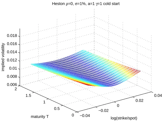
We assume that the evolution starts at t0 = 0 from some arbitrary valuex0. The standard “cold-start” setup also includes the initial value for the stochastic variance factor z0, the simplest default choice beingz0= 1. An example of the implied volatility surface is presented in Figure1. As expected, at short maturities the smile is weak. This is because the fluctuations of the volatility are not fully active during the initial relaxation period, which is of the ordera−1= 1 here.
3
Choice of the Hot-Start Distribution
−0.04 −0.02
0
0.02 0.04
0 0.5 1 1.5 2 0.006 0.008 0.01 0.012 0.014 0.016 0.018
log(strike/spot)
Heston ρ=0, σ=1%, a=1 γ=1 cold start
maturity T
[image:24.612.162.448.95.308.2]implied volatility
Figure 1: Implied volatility surface for a cold-start (z0= 1) Heston model.
for the evolution of the stochastic multiplier z, assuming that it has actually started much earlier and reached its equilibrium Gamma distribution with the density
Fa,γ(z) = α
α
Γ(α)z
α−1exp[−αz], (3.1)
α= 2
aγ2.
by the timet0= 0. This straightforward choice may be quite a practical approximation in many cases. However, a more rigorous setup is also worth discussing.
In reality, some indirect information about the latent part of the process is available through the known history of the observable path because these components are coupled. Thus, we can expect that the hot-start distribution may be shifted and somewhat squeezed with respect to the equilibrium one. The question is how to quantify this effect. In the spirit of standard calibration, we are allowed to assume that today’s market absorbs historical information and translates it into quotes. Under such an assumption, it is enough to somehow parameterize today’s distribution of the latent factor and to calibrate these parameters together with those of the process.
Since the estimation cannot be very accurate in general, it should be sufficient to use only a couple of parameters related to the moments of the distribution. The “historical” effects we are trying to adapt to are not able to drastically change the principal features of the distribution. It is therefore most suitable to use the distribution from the same family as the equilibrium one.
For the Heston model, we suggest the Gamma distribution
F(z) = z
α−1
Γ(α)βαexp [
−z β ]
(3.2)
with two parameters: the shapeαand the scaleβ. The moment generating function is
correspond to the unit average ofz,
E[z] = 1,
and the variance
E[(z−z¯)2] =αβ2=α−01=aγ
2
2 .
We introduce two scaling parameters ζand ω, determined by
α=α0
ω ,
β =ζω
α0 ,
so that the average value ofz and its variance become
E[z] =αβ=ζ
and
E[(z−z¯)2] =αβ2=ωζ
2
α0
=ωζ2aγ 2
2 ,
respectively. The idea of this choice of scaling is that the bare equilibrium setting is obtained simply by setting ζ=ω= 1, and adjusting the average value ofz through theζ parameter does not perturb the shape αof the distribution.
When the model is applied in the econometric context, we do not usually rely on today’s market quotes. Instead, we have to explicitly analyze the historical time series by considering the latent distri-bution to be a result of a long evolution, conditional on the actually recorded history of the observable variables. An accurate determination of the conditional distribution is a very challenging task. In fact, it is very close to the maximum likelihood estimation of multifactor process parameters from the historical market observables. It cannot be accomplished exactly, but there are workable approximations based on a recursive forward-in-time buildup of a few (e.g., two) of the lowest moments of the distribution. Once the recursion reaches the end (today), the hot-start distribution can be adjusted to match the obtained moments. In the case of the Heston process, the derivations are available, for instance, from Hurn et al. [6] and references therein. The parameterization introduced above is naturally valid for this purpose as well.
Computational Aspects
The complication introduced by the hot-start initialization to any computational framework is minimal because the underlying stochastic process remains the same.
The most straightforward is an extension of Monte Carlo simulation. Instead of initializing all the simulation paths by the same fixed value of the latent variable, the initial value should be sampled from the adjusted distribution. Essentially, this is equivalent to inserting a special Monte Carlo step at today’s time node. The statistical accuracy of the pricing should not deteriorate.
In a finite difference scheme, the price is usually obtained by taking the payoff at the spot node of the lattice after back propagation to today’s time node. For the hot-start evaluation, the payoff must be collected from the entire projection of the latent variable grid with the given spot value of the observable variable and averaged with the adjusted distribution.
−0.04 −0.02
0
0.02 0.04
0 0.5 1 1.5 2 0.006 0.008 0.01 0.012 0.014 0.016 0.018
log(strike/spot)
Heston ρ=0, σ=1%, a=1 γ=1 hot start
maturity T
[image:26.612.163.447.96.309.2]implied volatility
Figure 2: Implied volatility surface for a Heston model with a hot-start initialization
from the equilibrium distribution (3.1).
As an example, for the same process parameters as those used for Figure 1, we applied the hot-start initialization with the full equilibrium distribution (3.1) and obtained the implied volatility surface shown in Figure 2. As expected, the surface changes only slightly on the horizons after the relaxation period a−1, but the smile gets stronger at early maturities and demonstrates a tendency to diverge at very short ones. This is in striking contrast to the cold-start case, where implied volatility remains finite in the limit of zero time to maturityT →0. (See, e.g., [3].)
Note also that the short-maturity smile depends on the reversion speeda. When the reversion spreed increases, both the cold-start and the hot-start volatility surfaces display more extreme smiles at short maturities and become indistinguishable in the limita→ ∞. This behavior was explored in [7]. Figure 3 provides a plot of the implied volatility of a such a fast-reversion Heston model.
Considering the short maturity asymptotic quantitatively, we notice that this limit reduces to pricing European options by the Black-Scholes model that corresponds to the first SDE in (2.2) with a fixed value of the factorz and averaging the result over the hot-start distribution (3.2). For a call option on the stock with spot value S0 and strikeK=S0exp[X+rT], the Black-Scholes priceCz(X)is
S0−1Cz(X) = e
−rT
2π
1
√
2πV ∫ +∞
X
exp
[ −
(
x+12σ2zT)2
2σ2zT ]
(
ex−eX)dx.
In the limit asT →0, it is enough to work in the main exponential approximation for the Black-Scholes out-of-the-money price
S0−1Cz(X)≈exp [
− X2
2σ2zT ]
and for the tail of Gamma distribution
F(z)≈e−z/β.
−0.04 −0.02
0
0.02 0.04
0 0.5 1 1.5 2 0.006 0.008 0.01 0.012 0.014 0.016 0.018
log(strike/spot)
Heston ρ=0, σ=1%, a=∞γ=1
maturity T
[image:27.612.164.447.98.307.2]implied volatility
Figure 3: Implied volatility surface for a fast-reversion Heston model (a=∞).
volatility ˜σ,
C(X)≈S0exp
[ − X2
2˜σ2T ]
.
A match is obtained for
˜
σ2=σ √
β
2T |X|,
where we included the symmetric result for in-the-money strikes.
We see that the implied volatility indeed diverges at short maturities asT−1/4. In addition, we see
that, like the fast-reversion limit of the Heston model, the hot-start volatility surface is symmetric on short maturities. This is natural, because the hot-start distribution effectively comes from the past and thus is not correlated with subsequent stochastic moves of the stock. Note that only the leading term is symmetric and the overall smile is significantly skewed even at rather short maturities, as demonstrated in Figure4.
4
Concluding Remarks
We see that the effect of hot-start initialization is very significant and suggest that it should be considered as an essential component of every model that contains latent stochastic factors. Specifically to the Heston model, we proposed the two-parameter distribution (3.2), which should be easy to calibrate to market options or to adjust to historical data in the maximum likelihood sense. We wish to stress once more that, even when there is not enough information to calibrate all parameters, the single-value initialization of the latent process is still a poor solution compared to the full-equilibrium hot-start initialization (3.1).
−0.04 −0.02
0
0.02 0.04
0 0.5 1 1.5 2 0.005 0.01 0.015 0.02
log(strike/spot)
Heston ρ=0.8, σ=1%, a=1 γ=1 hot start
maturity T
[image:28.612.164.448.96.308.2]implied volatility
Figure 4: Implied volatility surface for a hot-start Heston model with strong correlation
between the stock and the volatility multiplier.
References
[1] Ballestra, L., Ferri, R., and Pacelli, G. The Heston stochastic volatility model for single assets and for asset portfolios: parameter estimation and an application to the Italian financial market. The International Journal of Business and Finance Research 1, 2 (2007), 11–23.
[2] Dragulescu, A., and Yakovenko, V. Probability distribution of returns in the Heston model with stochastic volatility. Quantitative Finance 2 (2002), 443–453.
[3] Forde, M., and Jacquier, A. Small-time asymptotics for implied volatility under the Heston model. IJTAF 12, 6 (2009), 861–876.
[4] Gatheral, J. The Volatility Surface: A Practitioner’s Guide. Wiley Finance, 2006.
[5] Heston, S. A closed-form solution for options with stochastic volatility with application to bond and currency options. Review of Financial Studies 6 (1993), 327–343.
[6] Hurn, A., Lindsay, K., and McClelland, A. A quasi-maximum likelihood method for estimat-ing the parameters of multivariate diffusions. Review of Financial Studies 172(2013), 106–126. [7] Mechkov, S. Fast-reversion limit of the Heston mode. Available athttp://ssrn.com/abstract=