On the probability distribution function of small-scale interplanetary magnetic field fluctuations

SRef-ID: 1432-0576/ag/2004-22-3751 © European Geosciences Union 2004

Annales

Geophysicae

On the probability distribution function of small-scale

interplanetary magnetic field fluctuations

R. Bruno1, V. Carbone2, L. Primavera2, F. Malara2, L. Sorriso–Valvo2, B. Bavassano1, and P. Veltri2 1_{Istituto Fisica Spazio Interplanetario del CNR, 00133 Roma, Italy}

2_{Dipartimento di Fisica Universit`a della Calabria, 87036 Rende (Cs), Italy}

Received: 10 May 2004 – Revised: 8 July 2004 – Accepted: 16 August 2004 – Published: 3 November 2004

Abstract. In spite of a large number of papers dedicated to the study of MHD turbulence in the solar wind there are still some simple questions which have never been sufficiently addressed, such as:

a) Do we really know how the magnetic field vector orien-tation fluctuates in space? b) What are the statistics followed by the orientation of the vector itself? c) Do the statistics change as the wind expands into the interplanetary space?

A better understanding of these points can help us to better characterize the nature of interplanetary fluctuations and can provide useful hints to investigators who try to numerically simulate MHD turbulence.

This work follows a recent paper presented by some of the authors which shows that these fluctuations might resemble a sort of random walk governed by Truncated L´evy Flight statistics. However, the limited statistics used in that paper did not allow for final conclusions but only speculative hy-potheses. In this work we aim to address the same problem using more robust statistics which, on the one hand, forces us not to consider velocity fluctuations but, on the other hand, allows us to establish the nature of the governing statistics of magnetic fluctuations with more confidence.

In addition, we show how features similar to those found in the present statistical analysis for the fast speed streams of solar wind are qualitatively recovered in numerical simula-tions of the parametric instability. This might offer an alter-native viewpoint for interpreting the questions raised above.

Key words. Interplanetary physics (interplanetary magnetic fields) – Space plasma physics (waves and instabilities)

1 Introduction

The first turbulent model proposed by Kolmogorov (1941) didn’t take into account that the rate of energy transfer along the turbulent cascade might not be scale-independent (Lan-dau’s objection). This situation, in the framework of a classi-Correspondence to: R. Bruno

([email protected])

cal Richardson’s cascade, can be described by the fact that smaller and smaller eddies are less and less space-filling. In other words, turbulence would be unevenly or intermit-tently distributed in space. As a matter of fact, we ad-dress this phenomenon as Intermittency. Evidence of the presence of this phenomenon, when performing a statistical study on a generic fluctuating fieldV (x), is that the probabil-ity distribution functions (PDF hereafter) of the differences

δvl(x)=|V (x+l)−V (x)|normalized to theσof the

distribu-tion at scaleldo not rescale for different scales (Van Atta and Park, 1975).

In particular, the tails of these PDFs become more and more stretched at smaller and smaller scales. This means that the wings of the distributions become fatter and fatter. Such behaviour implies that, at smaller scales, extreme events be-come statistically more probable than if they were normally distributed.

tool to finally disclose the nature of intermittent events. In this last paper, the authors showed that the intermittent event they were able to single out was a so-called current-sheet-associated TD, as defined by Ho et al. (1995). This type of structure is associated with wind velocity gradients, a rapid magnetic field intensity change and a reversal of the maxi-mum variance magnetic field component across the discon-tinuity, which was interpreted as the interface between two adjacent flux tubes, i.e. two regions characterized by differ-ent plasma and magnetic field conditions although within the same large-scale plasma region. During these studies, it was also noticed that the jumps performed by the tips of magnetic and velocity vectors resemble a typical L´evy process (Bruno et al., 2004). This process is similar to a random walk but the statistics governing the spatial jumps are characterized by ex-treme behaviour. Consequently, the presence of long-range correlations makes the Gaussian statistics, which govern the Brownian motion, no longer representative of the physical process. In fact, the spatial distribution of the directions as-sumed by these vectors during the selected time interval was not uniform but rather patchy. This particular behavior in-dicates the presence of particular directions along which the fluctuating field vector would roughly remain aligned for a longer time. Then, a rapid and large jump would charac-terize the transfer from one patch to another. These large jumps were recognized to make the fluctuating field more intermittent. Moreover, the highly Alfv´enic character of the selected time interval clearly showed that propagating modes and coherent structures were both contributing to the observed turbulence and strengthened the already proposed view of a turbulence made of a mixture of waves and struc-tures (Matthaeus et al., 1990; Bruno and Bavassano, 1991; Tu and Marsch, 1991; Marsch and Liu, 1993; Tu and Marsch, 1993; Klein et al., 1993, among others). In reality, it took a long time to reach this view of interplanetary MHD turbu-lence. As a matter of fact, the first spectra of solar wind fluc-tuations obtained from the observations of Mariner 2 in 1962. were interpreted by Coleman (1968) as evidence for the pres-ence of turbulent processes, possibly MHD turbulpres-ence as de-scribed by Kraichnan (1965). The velocity shear mechanism proposed by Coleman (1968) would be sustained by strong velocity gradients present in the solar wind and would pro-duce large-scale Alfv´en waves that would transfer their en-ergy to smaller and smaller scales through a turbulent pro-cess. On the other hand, Belcher and Davis (1971), looking at the correlation between velocity and magnetic field fluctu-ations observed by Mariner 5, concluded that interplanetary fluctuations were exclusively made of outward propagating Alfv´en modes, mostly of solar origin. Obviously, these two points of view were in contradiction because the absence of inward propagating modes would preclude the development of a turbulent cascade of energy to form a spectrum similar to the one observed by Coleman (1968). In reality, interplan-etary fluctuations are not just Alfv´en waves. Only several years later, a careful data analysis performed on the observa-tions provided by the Helios spacecraft contributed to make the idea of a possible coexistence of propagating waves and

convected structures accepted (see review by Tu and Marsch, 1995). Moreover, only recently, theoretical efforts (Wu and Chang ,2000; Vasquez and Hollweg, 2004; Vasquez et al., 2004) have shown the possibility that propagating modes and coherent structures might share a common origin within the general view described by the physics of complexity. Prop-agating modes would experience resonances which generate coherent structures which, in turn, will migrate, interact and eventually generate new modes. Moreover, Primavera et al. (2003), using a 1-D MHD numerical simulations based on a pseudo-spectral code, were able to qualitatively reproduce the radial behavior of magnetic field and velocity Intermit-tency observed by Bruno et al. (2003) in the inner helio-sphere. In particular, they numerically simulated the prop-agation of a turbulent Alfv´enic spectrum in a uniform back-ground magnetic field. As a matter of fact, coherent struc-tures were created during the spectral evolution due to the parametric instability resembling a sort of shocklet or cur-rent sheet. Obviously, the model has strong limitations since while the 1-D code allows for dependence on only 1 spatial coordinate, the vectors can have all 3 Cartesian components. As a consequence, these results remain at a qualitative level. Using the idea of McCracken and Ness (1966) as a start-ing point, Bruno et al. (2001) proposed the spaghetti-like model in which Alfv´enic fluctuations propagate within a con-vected structure made of tangled flux tubes, each of them be-ing characterized by their local magnetic field and plasma. These structures represent the correlated part of the signal, unlike from the Alfv´enic component which does not con-serve spatio-temporal coherence.

Moreover, it was found that the statistics associated with these fluctuations experienced a strong radial evolution. As a matter of fact, directional jumps, within fast solar wind, evolved from a more Gaussian-like statistic at 0.3 AU to-wards a sort of Truncated L´evy Flight (Mantegna, 1994) statistic at 0.9 AU. This phenomenon suggested that the pos-sible cause of the radial evolution was the radial progressive depletion of the Alfv´enic component of the turbulent fluctu-ations with respect to the convected structure. However, the limited statistics due to the low resolution of plasma data did not allow for a more refined analysis. In this paper we used higher resolution data, about one order of magnitude higher in frequency, to study in more detail the structure of the PDFs of directional fluctuations but we had to limit this study to the only magnetic component of the fluctuations.

2 Data analysis

→ → → → → →→ →

!"

#

$

%

!&

'

(

$

'

)

*

+

!

γ

$

+ *

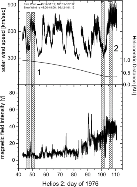
Fig. 1. Top panel: solar wind speed profile versus time as recorded

during the first solar mission of Helios 2. The solid, smooth line represents the heliocentric distance of the s/c which varied between 0.97 and 0.29 AU. Bottom panel: magnetic field intensity profile versus time. The whole interval was characterized by the presence of only one shock around day 90. Vertical hatched regions identify time intervals chosen for this analysis. There are two high speed intervals located in the trailing edge of two corotating streams and two low speed intervals ahead of them.

to study the radial evolution of interplanetary turbulence. As a matter of fact, this data set contains in-situ observations at different heliocentric distances of magnetic field and plasma belonging to the same corotating solar source region of high velocity wind. Thus, the stationary character of this region allowed for studies which could focus on the radial evolution of solar wind turbulence, providing extremely important re-sults which have been reviewed in an excellent paper by Tu and Marsch (1995). In the present analysis we will refer to this particular high velocity stream and to the low velocity wind ahead of it, observed at two different heliocentric dis-tances, namely 0.3 and 0.9 AU. These time intervals are high-lighted in Fig. 1 by vertical hatched stripes which, from the top to the bottom of the figure, go across velocity and helio-centric distance in the top panel and magnetic field intensity in the bottom panel. Each of the four time intervals lasts 2 days and has approximately 28 800 6-s averages, taking into account data gaps. Temporal extremes, average heliocentric

Table 1. Time extremes and average values characterizing the

in-tervals.

time interval distance <V > <B> (dd:hh) (AU) (km/s) (nT)

46:00–48:00 0.90 433 6.8 49:12–51:12 0.88 643 6.8 99:12–101:12 0.34 405 28.9 105:12–107:12 0.29 729 42.1

distance, average wind speed and field intensity are reported in Table 1 for each interval.

Just for sake of completeness we like to add that the same corotating stream was also observed at 0.7 AU start-ing around day 74 but we will omit that time interval since it would be redundant for the analysis we present here. As already stated in Sect. 1, the main goal of this work is the study and characterization of directional fluctuations. To do so, we start with plotting the position of the tip of the mag-netic field vector within the reference system of the three co-ordinate axes during sub-intervals of only 2000 points within the selected time periods. These sub-intervals can be con-sidered representative of each particular interval they refer to. A longer sequence of points would make it impossible, in the graphical format we used, to recognize the differences between different intervals.

Fig. 2. The top panel refers to a fast wind recorded at 0.3 AU while

the bottom panel refers to a fast wind at 0.9 AU. Each point of both plots represents the location of the tip of the magnetic field vector for each 6-s average. These locations have then been connected by a black straight line to form a trajectory. Moreover, the shadow of this trajectory is also shown on the three coordinate planes to better understand the spatial 3-D configuration. In these panels we show only intervals of 2000-point representing larger intervals of 28 800 6-s averages. Values of each component have been nor-malized to the average magnetic field intensity measured within the 2000 points interval. The top panel shows a more uniform coverage with respect to the bottom panel, which shows a sort of patchy con-figuration. In other words, there is some kind of evolution during the radial expansion which is dramatically reflected in this kind of spatial behaviour.

still wanders on the surface of only half a sphere, it does not cover this surface completely but leaves out wide areas. The distribution of the dark spots suggests that the presence of preferred spatial directions, connected by large and quick jumps which take only a few data points, begins to emerge as the heliocentric distance increases.

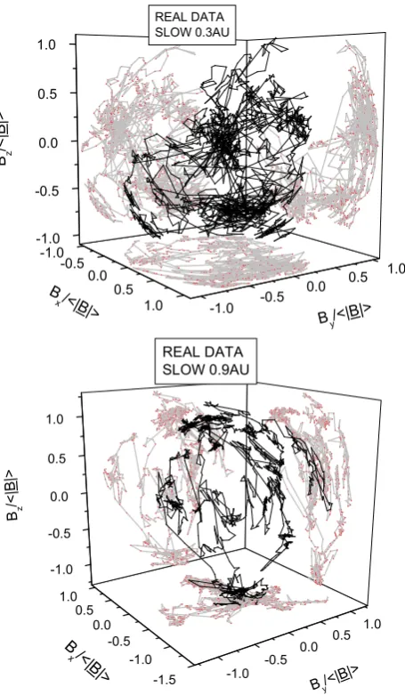
Fig. 3. The top panel refers to a slow wind recorded at 0.3 AU while the bottom panel refers to slow wind at 0.9 AU. The format is the same used for Fig. 2 and, also in this case, we show only 2000 points out of 28 800 points of each selected time interval. Both configurations relative to 0.3 and 0.9 AU greatly differ from what we observed within fast wind. In both cases a patchy configuration is clearly visible, meaning that the tip of the vector dawdles longer around some particular orientation. At first sight, the two panels show similar configurations, although fluctuations at 0.3 AU appear to be slightly larger. Definitely, we do not observe the same radial evolution noticed for a fast wind.

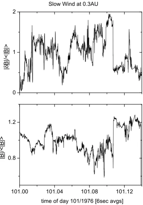
However, this kind of graphical representation is not suffi-cient to give an idea of how the tip of the vector really moves in time unless complemented by the information we provide in the top panel of Fig. 4. In this panel we show the vector displacement|δB(t )|, normalized to<|B|>, between each

B(t )and an arbitrary fixed direction which we chose to be the direction of the first vectorB(t0)of the time series. Thus, following this definition, each individual|δB(t )|is given by:

|δB(t )| =

s X

i=x,y,z

(Bi(t )−Bi(t0))2. (1)

This time sequence, the same used for the top panel of Fig. 3 which refers to a slow wind at 0.3 AU, clearly shows a small amplitude and high frequency fluctuations superimposed on a sort of larger amplitude low-frequency background struc-ture. This background structure is characterized by a few large and quick directional jumps. The effect of these jumps is to move the fluctuating vector from one particular aver-age direction to another, i.e. from one dark spot to another (Fig. 3). This type of information, together with the 3-D graphical representation, gives an idea of how the vector di-rection really fluctuates in space and time. Moreover, most of the time the largest directional jumps are associated with the largest changes in the field intensity (bottom panel). So, these two panels suggest that during short time intervals the field can be characterized by a most probable orientation and a most probable intensity. In other words, these regions ap-pear to be distinguishable from each other and the transition from one to another is through a large rotational jump and a change in the field intensity. Similar findings have already been reported in a previous paper (Bruno et al., 2001), al-though it was focused on a single case study and on larger scales. In that same study it was found that this kind of transi-tion, or border, was a tangential discontinuity not in pressure balance. The features we notice in the present study might be TDs as well, although we cannot prove it since we don’t have plasma data with the same time resolution of magnetic field data. If this is the case, the structure we have seen at larger scales replicates at smaller scales in a kind of self-similar manner.

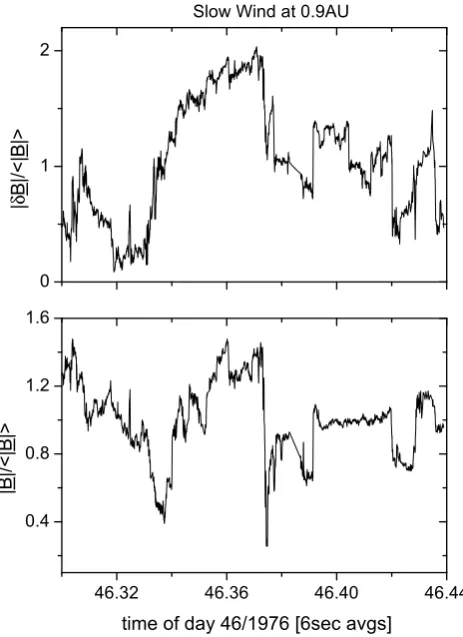
Results relative to a slow wind at 0.9 AU are shown in Fig. 5 in the same format as the previous figure. Although, both panels show fluctuations generally smaller than the cor-responding ones observed at 0.3 AU, corcor-responding features in both profiles are still clearly recognizable. Thus, radial evolution within slow wind doesn’t play much of an influ-ence on this kind of relationship.

In Fig. 6 we show vector displacement for the time inter-val recorded at 0.3 AU, within a fast wind in the same format as the previous two figures. Directional fluctuations appear to be very chaotic and not as much structured as we found in the slow wind. Thus, it is certainly more difficult to recog-nize structures similar to the ones observed in the previous figures and correlate them to the profile of the magnetic field intensity in the bottom panel. As a matter of fact, we expect to find large amplitude directional fluctuations within a fast

! " # $%&

δ

Fig. 4. Data refer to a slow wind at 0.3 AU. Top panel: vector

dis-placement|δB(t )|, normalized to<|B|>, between eachB(t )and an arbitrary fixed direction versus time. The arbitrary direction was chosen as the direction of the first vector of the time series. This kind of graph shows a series of time intervals during which the vec-tor displacement tends to remain approximately close to the aver-age level. These time intervals are interleaved by large and quick directional jumps. Moreover, the largest jumps often coincide with remarkable changes in field intensity as shown in the bottom panel.

wind, especially close to the Sun, because we are aware of the relevant presence of Alfv´enic modes in this type of wind. As a consequence, we believe that these fluctuations mask the correspondence we were able to highlight within a slow wind which, a priori, might be similar to that. Consequently, if the Alfv´enic modes had a smaller amplitude, we would be able to recognize and relate similar features in both panels.

δ

! " # $%"&

Fig. 5. Vector displacement versus time in the same format as of Fig. 4 relative to a slow wind at 0.9 AU. Largest vector displace-ments (top panel) often coincide with large compressive events, as shown in the bottom panel. As shown in the paper, the statistics of these vector displacements is remarkably similar to that shown in the previous Fig. 4

.

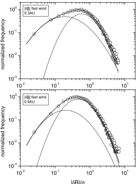
This qualitative study has to be substantiated with some quantitative evaluation of the relative importance of these two components contributing to the observed interplanetary turbulence. To do so, in the following, we will discuss and compare the probability distribution functions (PDF) of the directional fluctuations observed within each time interval. In order to look for a possible scaling between different PDFs, we have normalized each|δB(t )|to the standard devi-ationσ of the relative distribution. Moreover, the maximum amplitude of each PDF was normalized to 1. In Fig. 8 we show PDFs for the fast wind samples recorded at 0.3 and 0.9 AU in the top and bottom panels, respectively. We found that both distributions can be reasonably well fitted by a dou-ble lognormal distribution in the form reported by Eq. (2).

P (ξ )= A1 σ1ξ

√ 2π exp

"

−

_{ln|ξ /δ}

1| √

2σ1

2#

+ A2 σ2ξ

√ 2π

exp

"

−

_{ln|ξ /δ}

2| √

2σ2

2#

(2)

δ

! " #$ %

Fig. 6. Fast wind at 0.3 AU. Normalized vector displacements

ver-sus time in the same format as Figs. 4 and 5, shown in the top panel, while normalized vector intensities are shown in the bottom panel. The top panel shows large fluctuations which are difficult to relate to the profile of the magnetic field intensity in the bottom panel, al-though some corresponding events can still be recognized. In this sense, fast wind at 0.3 AU differs from the slow wind samples we already discussed.

where ξ, δ, σ >0. The variable ξ stands for the different |δB_i|/σ, one for each bin of the distribution,Ai is a

mea-sure of the area under each curve, δi is called a scale

pa-rameter and represents the median,σi is the shape parameter.

Larger values of σi push the x-location of the peak of the

distribution towards lower values. Obviously, using a larger number of lognormals would provide a better fit but, the real conspicuous improvement is obtained only when we use two lognormals instead of just one.

!"

δ

Fig. 7. Normalized vector displacements and normalized vector

in-tensity versus time are shown in the same format of Figs. 4–6 for a fast wind at 0.9 AU. Vector displacements shown in the top panel appear to be less chaotic than those observed at 0.3 AU. A sort of underlying structure can be recognized and related to field inten-sity fluctuations shown in the bottom panel. In other words, this situation tends to resemble the one encountered within slow wind.

peaked on smaller|δB|/σstrongly decreases its contribution with increasing radial distance from the Sun. An estimate of this evolution can be inferred from the ratio of the areas A1and A2 below each curve. While at 0.3 AU the proba-bility ratioA2/A1'0.52, at 0.9 AU it drops to'0.22. Con-sequently, the contribution of the smaller PDF to the whole PDF varies from 34% at 0.3 AU to 18% at 0.9 AU. All the other parameters do not experience a similar radial variation, and this behavior reflects in a depletion of the left-hand tail of the total PDF. However, it is worth noticing that both val-ues ofδare located at somewhat larger values for the sample referring at 0.3 AU, suggesting that fluctuations are generally larger when closer to the Sun.

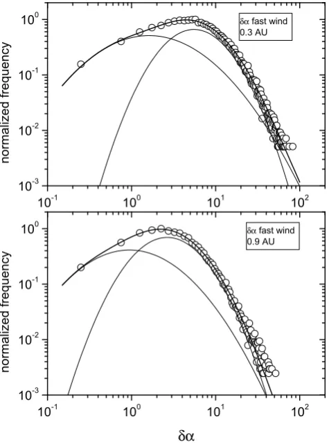
Similar conclusions apply to the PDFs relative to the an-gular fluctuationsδα experienced by the vector orientation shown in Fig. 9. Obviously, this measure provides informa-tion only about direcinforma-tional fluctuainforma-tions and is not influenced by compressive effects that may act on the vector intensity. As such, information contained in Fig. 9 is less meaningful than that discussed earlier but we like to show this kind of

fig-δ σ

δ δ

Fig. 8. PDFs of vector displacements|δB|normalized toσ at 0.3 and 0.9 AU, for a fast wind, are shown in the top and bottom panels, respectively. The two thin solid curves refer to as many lognormals contributing to form the thick solid curve which best fit the distri-bution. Parameters relative to the fit are reported in Table 2.

ure, and the analogous one for a slow wind in Fig. 11, just for sake of completeness. Moreover, these distributions have not been normalized to their respectiveσ valves since we like to show the effective angular range of these fluctuations. Also, for this fit we report the relative parameters which are shown in Table 3. For these fluctuations the ratio A2/A1varies from 56% at 0.3 AU to 40% at 0.9 AU. The PDF is clearly peaked at larger angles (5.75◦_{compared to 2.25}◦_{) at 0.3 AU and its}

right tail reaches values close to 100◦.

δα

δα

δα

Fig. 9. PDFs of angular displacementsδαat 0.3 and 0.9 AU, for a fast wind, are shown in the top and bottom panels, respectively. The two thin solid curves refer to as many lognormals contributing to form the thick solid curve which best fit the distribution. Parameters relative to the fit are reported in Table 3.

parameters inferred from the fit of the main lognormal, is re-markable which highlights the absence of radial evolution. In this case, values ofδare considerably smaller than those obtained for a fast wind, confirming that these fluctuations are generally smaller.

As already reported for a fast wind, we like to show the PDFs relative to the angular fluctuations as shown in Fig. 11, and parameters relative to the best fit, which are shown in Ta-ble 5. Also in this case, the contribution of the smaller log-normal is much smaller than within a fast wind. As a matter of fact, the ratio A2/A1varies from 7.5% at 0.3 AU to 4.4% at 0.9 AU. Moreover, these PDFs are roughly peaked at the same angle (0.75◦), although the right tail at 0.3 AU reaches larger values and does not show any noteworthy radial de-pendence.

2.1 Building artificial interplanetary time series

At this point, we tried to reproduce, from a statistical point of view, our interplanetary data samples by employing a ran-dom walk process governed by a double lognormal statistic acting on the direction of a unit vector. In other words, the

δ

δ σ

δ

Fig. 10. PDFs of vector displacements|δB| normalized toσ at 0.3 and 0.9 AU, for a slow wind, are shown in the top and bottom panels, respectively. The two thin solid curves refer to as many lognormals contributing to form the thick solid curve which best fits the distribution. Parameters relative to the fit are reported in Table 4. The smaller lognormal is almost superfluous since its contribution to the final fit is negligible.

interval of variability of|δB_i|, as inferred from real data, was divided into a sufficient number of bins. For each of them we generated a certain number of values, all equal to the value represented by the mid point of the bin. The number of val-ues generated depended on the corresponding probability in-dicated by the double lognormal, which was shaped using the same parameters that we had previously obtained from our best fits and reported in Tables 2 and 4. These|δB_i|were then randomly extracted and used to make the tip of a unit vector, with one end fixed at the center of a sphere of unit radius and the other end free floating on the surface of the sphere. The direction of the path followed by the tip of the vector at each step was randomly extracted between 0◦and 360◦. In particular, to avoid the effect of the two singular points at the poles of the sphere, the Cartesian coordinates of our reference system were rotated after each extraction in order to have the x axis always coinciding with the newly extracted direction.

δα

δα δα

Fig. 11. PDFs of angular displacementsδαat 0.3 and 0.9 AU, for a slow wind, are shown in the top and bottom panels, respectively. The two thin solid curves refer to as many lognormals contributing to form the thick solid curve which best fit the distribution. Param-eters relative to the fit are reported in Table 5. Also in this case, the contribution of the smaller lognormal to the final fit is negligible.

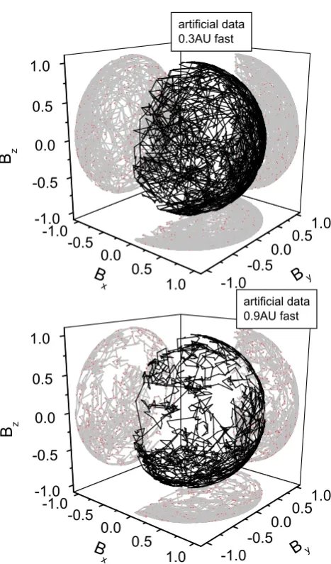
and 0.9 AU, for a fast and a slow wind were built in such a way. Samples of 2000 data points each are plotted in Fig. 12 and Fig. 13, for a fast and a slow wind, respectively. The only arbitrary imposition we applied on the fast wind sample was that to always keep the same vector polarity to resemble, as much as possible, the real situation within a fast wind. As a consequence, we forced these fluctuations to remain within a solid angle of 2π aperture. These plots reproduce at some level the main features that can be observed in Figs. 2 and 3. Fluctuations appear more intermittent in slow wind but show the largest evolution, between 0.3 and 0.9 AU, within a fast wind. Obviously, all the artificial time series we built have, by definition, the same statistics of real interplanetary data and we omit showing the PDFs of the relative|δB_i|/σorδα. On the other hand, we like to show temporal sequences of these|δB(t )|relative to a fixed, arbitrary direction, as we did for real data shown in the top panels of Figs. 4 to 7. Only the top panels have to be considered, since artificial data have been built to keep the vector intensity constant. Results are quite satisfactory since we are able to reproduce the typi-cal behavior observed within both a fast and a slow wind.

Fig. 12. Three-dimensional representation of vector displacements

relative to artificial data generated by a random-walk, whose jumps obey a double-lognormal, whose parameters have been obtained by the best fit of real fluctuations. The top and bottom panels refer to fast wind at 0.9 and 0.3 AU, respectively, and have to be compared to analogous plots for real data shown in Fig. 2.

In particular, the transition from the chaotic behavior on the left panel of Fig. 14, representing fluctuations at 0.3 AU, to-wards more structured fluctuations on the right panel of the same figure, representing fluctuations at 0.9 AU, is well re-produced by the artificial time series.

Moreover, artificial data reproduce equally well fluctua-tions encountered at both heliocentric distances in a slow wind. They show similar structured fluctuations and not rel-evant differences between 0.3 and 0.9 AU.

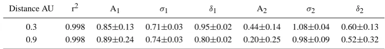
Table 2. Fast Wind: Values of the parameters obtained from the fit of the PDF relative to vector displacements.

Distance AU r2 A1 σ1 δ1 A2 σ2 δ2

0.3 0.998 0.85±0.13 0.71±0.03 0.95±0.02 0.44±0.14 1.08±0.04 0.60±0.13 0.9 0.998 0.89±0.24 0.74±0.03 0.80±0.02 0.20±0.25 0.98±0.09 0.52±0.32

Table 3. Fast Wind: Values of the parameters obtained from the fit of the PDF relative to angular fluctuations.

Distance AU r2 A₁ σ₁ α₁ A₂ σ₂ α₂

0.3 0.998 8.47±0.76 0.72±0.02 9.24±0.14 4.77±0.84 1.16±0.03 6.28±0.81 0.9 0.999 4.62±0.78 0.75±0.03 4.67±0.09 1.87±0.82 1.07±0.05 3.00±0.82

Fig. 16, where power spectra relative to real fluctuations are reported in the left-hand panel while corresponding spectra of artificial time series are in the right-hand panel.

The power spectra of the components have been computed via a Fast Fourier Transform from time series of 2048 data points. The power spectral densities of the three components have been successively added up to obtain the trace of the spectral matrix which has been smoothed by averaging ad-jacent data points within a sliding window of 5 points. In the same panels we also show as a reference the slope of the classical Kolmogorov’s spectrum. Spectra shown in the left-hand panel are typical spectra encountered within high velocity streams, as several times reported in literature (see review by Tu and Marsch, 1995). On the other hand, artificial spectra have been graphically separated by multiplying the spectrum identified by the label 0.3 AU by a factor of 102to avoid overlapping. As a matter of fact, our artificial fluctua-tions have statistically similar amplitudes, no matter whether we refer to 0.3 or 0.9 AU, since our fluctuations are confined onto the surface of a sphere of unitary radius. Unexpect-edly, the resemblance is so good that the artificial spectrum at 0.3 AU shows a bending similar to the one that character-izes real fluctuations. The main differences seem to be in the high frequency tail of artificial data where effects due to aliasing, absent in the left-hand panel, can be noticed.

3 Results of the numerical simulations of parametric in-stability

Recently, Primavera et al. (1999); Malara et al. (2000, 2001); Primavera et al. (2003) investigated in detail how the para-metric instability could be responsible for typical features observed in the radial evolution of the Alfv´enic turbulence in the solar wind high speed streams. This instability develops in a compressible plasma and, in its simplest form, involves the decay of a large amplitude Alfv´en wave (generally called a “pump wave”, or “mother wave”) in a magnetosonic fluc-tuation and a backscattered Alfv´en wave. The wavevectors

Table 4. Slow Wind: Values of the parameters obtained from the fit of the PDF relative to vector displacements.

Distance AU r2 A1 σ1 δ1 A2 σ2 δ2

0.3 0.998 0.776±0.003 0.959±0.009 0.523±0.004 0.002±0.001 0.437±0.095 0.039±0.010 0.9 0.998 0.727±0.004 0.934±0.005 0.503±0.004 0.001±0.001 0.532±0.722 0.049±0.009

Table 5. Slow Wind: Values of the parameters obtained from the fit of the PDF relative to angular fluctuations.

Distance AU r2 A1 σ1 α1 A2 σ2 α2

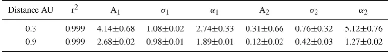
0.3 0.999 4.14±0.68 1.08±0.02 2.74±0.33 0.31±0.66 0.76±0.32 5.12±0.76 0.9 0.999 2.68±0.02 0.98±0.01 1.89±0.01 0.12±0.02 0.42±0.03 1.27±0.02

(see review by Tu and Marsch, 1995). In addition, Malara et al. (2000) observed that the turbulent development of the instability leads to the formation of shock waves and to an in-termittent behaviour of the dissipation. In particular, looking at the evolution of the flatness of velocity and magnetic field fluctuations, Primavera et al. (2003) found a good qualitative agreement of the results of the simulations with the analysis of the same quantities performed by Bruno et al. (2003). It is then natural, in order to offer a possible different interpre-tation of the results shown in the previous sections, at least those concerning fast solar wind streams, to see whether tur-bulence induced by parametric instability has characteristics similar to those described in the solar wind in the previous sections. To accomplish this aim, we further analysed the re-sults of the numerical simulations described in Primavera et al. (2003). The details of the numerical code can be found in Primavera et al. (1999), Malara et al. (2000) and Malara et al. (2001), whilst further details concerning the simulations are given in Primavera et al. (2003).

We simulate the evolution of a broad-band Alfv´enic fluctu-ations in a compressible plasma, during their outward propa-gation in the heliosphere. Similar to the in-situ observations, the initial spectrum has a break point. During the run of the simulation, inward propagating fluctuations start to appear and form a power-law spectrum at small values of k. As already pointed out by Tu et al. (1989), this feature might suggest that a parametric decay mechanism is at work in the solar wind.

The simulation domain is one-dimensional, periodic and we use Cartesian geometry.

The reference frame is chosen in such a way that the ini-tial Alfv´en wave is circularly polarized in thex−zplane and it propagates along they direction. A background constant magnetic field intensityB0is imposed in the propagation di-rection of the wave: the resulting total field has, therefore, uniform intensity everywhere.

The homogeneous boundary conditions limit the applica-tion of this study to the fast wind, where the background

magnetic field is rather homogeneous. In our framework, the time evolution of the quantities represents the radial evolu-tion of the fluctuaevolu-tions in the solar wind, while the spatial variations are the numerical counterpart of samples of the observed data at a given distance from the sun. We study the evolution of the parametric instability for 180τA(τA is the

Alfv´en time based on the initial background radial magnetic field and density, i.e. the time needed for the wave, whose wavelength is the largest in our spectral domain, to go across the simulation box). In the rest of the paper, we plot quanti-ties at timet1=45τAandt2=180τA, the former

correspond-ing to a time much before the saturation of the instability, the latter to a time longer than the saturation time, which is reached attsat∼100τA. Practically, we consider a situation in

which the instability has only weakly taken place and another in which it has already completely developed, that should be representative of the state of the solar wind closer to the Sun and further away from it, respectively.

We estimated the time needed by the instability to saturate and to reproduce the spectral features observed at 0.9 AU. We found that a period of time between 6 and 7 days is nec-essary. This estimation, although longer, is still within the same order of magnitude of the expansion time required by the solar wind to travel between 0.3 and 1 AU. The above evaluation is based on the fact that betweent1andtsatthere are about 55τA. In order to estimate τA we compared the

frequencies corresponding to the observed spectral break at 0.3 AU in Helios data with the corresponding one shown in our simulation att=t1.

In Fig. 17, we show the three-dimensional plots of the magnetic field components, normalized to the average mag-netic field intensity, at the timet1(upper panel) andt2(lower panel), respectively. These plots are to be compared to Fig. 2. One can see that att=45τAthe tip of the magnetic field

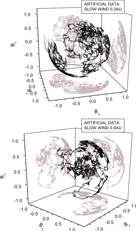
Fig. 13. Three-dimensional representation of vector displacements

relative to artificial data generated by a random-walk, whose jumps obey a double-lognormal, whose parameters have been obtained by the best fit of real fluctuations. The top and bottom panels refer to a slow wind at 0.9 and 0.3 AU, respectively, and have to be compared to analogous plots for real data shown in Fig. 3.

case, here the tip of the vector covers almost uniformly a cylinder instead of a sphere. This difference is due to the fact that the numerical simulation is one-dimensional: this implies (due to the divergenceless condition for the magnetic field) that the variations of the magnetic field components are only orthogonal to the propagation direction of the waves, whilst the parallel component remains constant during the time evolution. Moreover, since the initial perturbation is circularly polarized, the trajectory of the tip of the vector would describe a circular line. In order to improve the vi-sualization of the curve, to make it three-dimensional instead of two-dimensional, we replaced the constant component of the magnetic field with a linearly growing function between zero and one, that makes the tip of the vector stay on a cylin-drical surface. The real data are three-dimensional instead,

and the approximately constant field intensity produces the spherical pattern plotted in Fig. 2, as already explained in Sect. 2.

At the later time, t2=180τA, the situation changes

dra-matically. The tip of the magnetic field vector describes a more patchy pattern, characterized by large jumps, fol-lowed by smaller fluctuations around a single direction, and so on. This pattern is qualitatively similar to that observed in Fig. 2. In conclusion, results of parametric instability sim-ulation seem to account for the observed transition to a sort of L´evy walk observed in the real solar wind data (see also Bruno et al. (2004)).

As a second point of agreement with the observations, we plot the vector displacements |δB|, with respect to a fixed direction, normalized to the mean magnetic field intensity as a function of the independent variabley. We compute this quantity by considering the magnetic field at a given timet and evaluating the vector differences of its compo-nents with the fixed direction (0;1;0)in each simulation grid point. Since in our simulation the background mag-netic field has components B₀=(0;1;0), we are practically plotting the vector displacements of the magnetic field fluc-tuations. Finally, we compute the intensity of this vector in each point. The results of this computation are shown in the upper panel of Fig. 18 at the timet1=45τAand Fig. 19 at the

timet=180τA. Along with these curves, the magnetic field

intensities|B(y)|, normalized to its mean value, at the same times, are shown in the lower panels of the figures. These graphics should be compared with the ones in Figs. 6 and 7, where the analogous quantities are plotted for the fast solar wind at 0.3 and 0.9 AU, respectively.

Also in this case, the qualitative similarity between the results of the simulations and the observed solar wind data is remarkable. At the timet=t1, corresponding to 0.3 AU, the vector displacements have a quite random behaviour, al-though not as “noisy” as in Fig. 6, and no evident correlation between the vector displacements and the magnetic field in-tensity is observed. Note that the fluctuations of the magnetic field intensity are rather small at this time, due to the fact that the initial wave is circularly polarized.

On the converseside, in Fig. 19, the vector displacements of the magnetic field appear to be more structured, charac-terized by fast rotations of the vector, followed by smaller oscillations around the new position. Moreover, there exists a clear correlation between the strongest gradients of the vec-tor displacements and the ones of the magnetic field intensity, as already observed in the real solar wind fast streams.

Finally, we plotted in Fig. 20 the PDFs of vector displace-ments|δB_λ|, defined as

|δB_λ(x, t )| =

s X

i=x,y,z

(Bi(x+λ, t )−Bi(x, t ))2, (3)

δ !

δ

Fig. 14. Vector displacement versus time as measured from artificial data referring to a fast wind at 0.3 AU on the left panel and at 0.9 AU

on the right panel. These plots should be compared to the top panels of Figs. 6 and 7, respectively.

δ

!

"

δ

!

Fig. 15. Vector displacement versus time as measured from artificial data referring to a slow wind at 0.3 AU on the left panel and at 0.9 AU

on the right panel. These plots should be compared to the top panels of Figs. 4 and 5, respectively.

compute the PDFs in Sect. 2. However, in comparison with real data, where the resolution of 6 s still lies in the inertial range, in the simulations we have to take into account the fact that the smaller scales are affected by viscosity and dif-fusivity. Thus, we evaluated the vector differences at a length scaleλ=λmax/628, whereλmaxis the maximum wavelength excited at the beginning of the simulation, and equals the length of the simulation domain. This length scale is rather small, compared to the integral scale of the domain, but still in the inertial range of the spectrum.

The similarity with Fig. 8, where the PDFs of the vector displacements|δB| are shown for the fast wind at 0.3 and 0.9 AU, is evident. Also in this case, it is possible to fit ef-fectively the curves with two lognormal distributions and the trend is similar to that observed in the solar wind data. In fact, the two lognormal distributions have comparable heights at t=t1, while the population relative to the long vector displace-ments increases its importance at subsequent times (t=t2).

The parameters of the fits are shown in Table 6.

Another point of similarity with the analysis of real data regards the power spectrum. As a matter of fact, as already shown by Malara et al. (2000) and Malara et al. (2001), the power spectrum obtained from the trace of the spectral matrix of the Alfv´enic fluctuations, after the saturation of the para-metric instability has been reached, shows clear evidence of a power-law inertial range similar to the one observed in the Helios data at 0.9 AU.

!"#$#%# & ' "

(

(

*

"

)

+

,

- .

/

(

(

!0 & ' "

*

"

)

+

,

- .

Fig. 16. The left panel shows power spectra obtained from the trace of the spectral matrix relative to magnetic field fluctuations recorded at

0.3 and 0.9 AU by Helios 2 in 1976. Each time interval had 2048 averages of 6 s each and are the same sub-intervals used for Figs. 2, 6, 7. The right panel shows power spectra obtained from the trace of the spectral matrix relative to the artificial field fluctuations relative to 0.3 and 0.9 AU, built from a random walk whose jumps obey a double-lognormal distribution. Data relative to 0.3 AU have been multiplied by a factor of 102to facilitate visual comparison with real data shown in the left panel. It is worth noticing that artificial data, besides a general agreement with real data, are able to reproduce the bending of the power spectrum observed at 0.3 AU. Straight solid lines indicate the k−5/3 Kolmogorov slope.

Table 6. Numerical simulation: Values of the parameters obtained from the fit of the PDF relative to vector displacements.

Simulated time r2 A₁ σ1 δ1 A2 σ2 δ2

45τA 0.954 1.13±0.14 1.43±0.09 1.08±0.20 0.47±0.06 0.35±0.03 0.94±0.03

180τA 0.996 0.52±0.56 0.72±0.21 0.45±0.27 0.09±0.55 0.69±0.95 0.15±0.45

to that observed in the real data of the fast solar wind. We conclude that the parametric instability offers a possible al-ternative explanation of the observed data.

4 Conclusions

In this paper we focused on the statistics followed by inter-planetary magnetic field fluctuations on a 6-s time scale, well inside the MHD regime (Bavassano et al., 1982), as observed in solar wind turbulence between 0.3 and 0.9 AU. In particu-lar, we aimed to understand the spatio-temporal evolution of the magnetic field vector through the study of changes expe-rienced by both vector orientation and intensity. Several pre-vious works, which dealt with a statistical approach to this same problem, considered different aspects connected to di-rectional fluctuations as, for example, power associated with the fluctuations, their radial evolution, their anisotropy, the nature of the fluctuations, their generation mechanisms, and so on, but none of them, to our knowledge, has ever studied how and why the orientation of these fluctuations changes with time. There have been only a few attempts to study similar problems but always limited to single case studies (Nakagawa et al., 1989; Tu and Marsch, 1991; Tsurutani et

al., 1994; Riley et al., 1996; Bruno et al., 2001). The most recent statistical approach to the same problem is represented in a paper by Bruno et al. (2004), in which these authors con-cluded that the temporal evolution of the magnetic field and wind velocity vectors directions might follow a sort of L´evy walk. That paper, although based on larger time scales and on weak statistics, represents the first attempt to understand the influence due to propagating modes and convected struc-tures on the orientation of velocity and magnetic field vectors within MHD turbulence. Following this analysis and, using a more robust statistics, we found that PDFs of interplan-etary magnetic field vector differences within high velocity streams can be reasonably fitted by a double lognormal dis-tribution. In other words, vector differences, which are due to the two distinct contributions of directional uncompres-sive fluctuations and purely compresuncompres-sive fluctuations, can be separated into two distinct PDFs. Moreover, the lognormal nature of the PDFs might suggest a multiplicative process at the origin of these fluctuations, that is typical of a turbulent cascade.

Fig. 17. The top panel of the figure refers to the results of the

numer-ical simulations of parametric instability at timet=t1=45τA, while

the bottom panel refers to the the results at timet=t2=180τA. Each

point of both plots represents the location of the tip of the magnetic field vector in a point of the simulation domain, in the same format of Fig. 2, which the present figure should be compared with. The difference in the shape of the plots, cylindrical for this figure, spher-ical for Fig. 2, is explained in the text. Also in this case, the sim-ulated data att=t1, corresponding to the real data at 0.3 AU, have

a more uniform distribution on the cylindrical surface, whilst the data att=t2(to compare with real data at 0.9 AU) show long jumps,

followed by small amplitude oscillations around the new values.

Incidentally, the multiplicative cascade notion was in-troduced by Kolmogorov into his statistical theory (Kol-mogorov, 1941, 1962) of turbulence as a phenomenologi-cal framework to accomodate extreme behaviour observed in real turbulent fluids.

Another interesting feature of these distributions is that the two PDFs have a different weight since one of them, the one that represents the smallest|δB_i|is always consider-ably smaller than the other one. Moreover, while the smaller PDF does evolve with heliocentric distance, decreasing its

δ

! " # $ $ %

Fig. 18. Results of the numerical simulations of the parametric

instability at timet=t1=45τA. Normalized vector displacements

versus the spatial coordinateyare shown in the top panel, while normalized vector intensities are shown in the bottom panel. This figure should be compared with Fig. 6. The top panel shows large fluctuations which are basically uncorrelated with the profile of the magnetic field intensity in the bottom panel. This behaviour is qual-itatively similar to that observed in the fast wind at 0.3 AU (see Fig. 6)

.

to-δ

! " #

$

$! " #

Fig. 19. Normalized vector displacements and normalized vector

intensity versus position in the simulation box are shown in the same format as Fig. 18 for the results of the numerical simulations at timet=t2=180τA. A difference with the previous figure,

vec-tor displacements (top panel) appear to be more structured in space and some sort of correlation with the field intensity (bottom panel) can be recognized. This behaviour is qualitatively similar to that observed in fast solar wind at 0.9 AU (Fig. 7).

tal power associated with turbulence. Thus, we might asso-ciate our convected structures to the 2-D turbulence identified in the solar wind by Bieber et al. (1996) and Matthaeus et al. (1990), who modeled interplanetary magnetic turbulence made of slab and quasi-2-D turbulence only. However, the dominant 2-D magnetic turbulence is characterized by the fact that its wave vector results to be normal to the ambient magnetic field direction. As a consequence, we would ex-pect to see a radial evolution even stronger than the one we observed for the slab component which has its wave vectors parallel to the ambient field. As a matter of fact, the turbu-lent cascade acts preferably on wave numbers perpendicular to the ambient magnetic field direction, as suggested by the three-wave resonant interaction (Shebalin et al., 1983; Bon-deson , 1985). On the contrary, the dominant component of the turbulence observed by Helios is the least affected by the radial evolution and probably should not be identified with the 2-D turbulence. Another possibility is that the 2-D turbu-lence is mixed together with the slab turbuturbu-lence and is repre-sented by the smaller PDF which experiences the stronger

δ _λ σ

Fig. 20. PDFs of vector displacements |δB_λ|, at the scale λ=λmax/628, normalized to σ for the results of the numerical

simulations of the parametric instability at timet=t1=45τA and

t=t2=180τAare shown in the top and bottom panels, respectively.

The two thin solid curves refer to as many lognormals contributing to form the thick solid curve which best fits the distribution. Param-eters relative to the fit are reported in Table 6.

One more interesting observation regards the topology showed by these fluctuations within a fast and a slow wind. We showed that the trajectory, followed by the tip of the magnetic vector during its turbulent fluctuations, follows a structured path. This path appears more clearly when the PDF of|δB_i|can be fitted by a single lognormal, as in the case of slow wind, regardless of heliocentric distance. How-ever, within a fast wind this structured path can be more eas-ily observed by increasing the heliocentric distance, in con-currence with the depletion of the Alfv´enic fluctuations. In other words, Alfv´enic modes mask the underlying magnetic, quasi-static structure convected by the wind. The superpo-sition of these two types of fluctuations is such that the fi-nal motion is characterized by extreme behaviour. Referring to the 3-D representation used in this paper, the tip of the vector appears to be trapped within a certain solid angle for some time but occasionally it escapes this limited angular re-gion and quickly travels, in a few time steps, to finally end up in another angular region characterized by a different av-erage orientation. These large jumps should be accounted for by the larger PDF and should be related to similar large jumps studied by Bruno et al. (2001) and interpreted as tan-gential discontinuities marking the border between adjacent flux tubes. On the contrary, local fluctuations, clustering around certain average directions, should have an Alfv´enic nature and should be identified by the smaller PDF. These re-sults support and further corroborate the recently re-proposed spaghetti-like structure model (Bruno et al., 2001) first intro-duced, although in the context of cosmic ray modulation, by McCracken and Ness (1966), to describe interplanetary mag-netic field topology.

Finally, adopting a sort of feedback procedure, we cross-checked the soundness of our fitting scheme, showing that artificial data obtained from the tip of a vector that randomly walks on the surface of a sphere of a constant radius, per-forming directional jumps, which obey a double lognormal, provides results similar, in some aspects, to those observed in interplanetary space.

However, the interplanetary observations we have do not allow one to understand whether these structures come di-rectly from the Sun or are locally generated by some mecha-nism. Recent theoretical results by Primavera et al. (2003) showed that coherent structures responsible for the radial dependence of Intermittency, as observed in the solar wind (Bruno et al., 2003), might be locally created by the paramet-ric decay of Alfv´en waves. These authors showed that dur-ing the turbulent evolution, coherent structures, like shock-lets and/or current sheets, were continuously created when the instability was active.

In order to see whether a similar mechanism may account for the observed behaviour of the vector displacements and their statistics, we further analyzed in this paper the results of the simulations performed in Primavera et al. (2003). The results of this investigation show a fairly good agreement, at least under the qualitative point of view, between the simu-lations and the solar wind data: either the evolution of the tip of the magnetic field vector, or the correlation between

the vector displacement at a given scale with the magnetic field intensity fluctuations, or the evolution of the PDFs of the vector displacement in time, all show trends similar to those observed in the real fast solar wind data. Unfortunately, a direct quantitative comparison between the simulations and the data is difficult due to the limitations of the model.

However, this mechanism, which might be active within a fast wind, should be less effective within a slow wind, given the remarkable decoupling between the magnetic field and the velocity field within this type of wind (Klein et al., 1993). Nevertheless, the enticing nature of the parametric insta-bility in explaining the results comes from some well-defined fact: a) it is a well-defined mechanism of physical origin that induces a turbulent evolution in the plasma and not an unde-fined turbulence model; b) it is likely applicable to explain many general observed features of a fast solar wind, like the evolution of the spectra, the decrease of the Alfv´enic cor-relation during the propagation in the heliosphere, and so on (Primavera et al., 2003); c) the observed evolution of the vec-tor displacements and of their relative PDFs can be seen as a natural consequence of the formation of shocklets and dis-continuities in the wind, organized in a sort of coherent struc-ture, that explain the long jumps observed in the magnetic field and the structures in the vector displacements at larger distances from the Sun. In particular, the decrease with dis-tance of the lognormal component of the PDFs correlated to the Alfv´enic part of the turbulence, can be seen as the con-tinuous transfer of energy between the Alfv´enic and magne-tosonic components of the waves during the evolution of the instability. However, a definitive conclusion about this point needs further investigation.

Another recent theoretical effort by Chang et al. (2004) models MHD turbulence in a way that tends to the view and interpretation of the interplanetary observations we pre-sented in this paper, that is the existence of two different components both contributing to turbulence. The theoreti-cal model presented by these authors tells us that propagat-ing modes and coherent, convected structures are both neces-sary, inseparable ingredients of MHD turbulence, since they share a common origin within the general view described by the physics of complexity Chang (1999); Vasquez and Holl-weg (2004); Vasquez et al. (2004). Propagating modes expe-rience resonances which generate coherent structures which, in turn, will migrate, interact and eventually generate new modes.

These theoretical models, which favour the local genera-tion of coherent structures, fully complement the possible so-lar origin of the convected component of interplanetary MHD turbulence.

Acknowledgements. Magnetic field 6 s averages derive from the Rome-GSFC magnetic experiment onboard Helios 2 s/c. (PIs of the experiment wereF. Mariani and N. F. Ness)

References

Anselmet, F., Gagne, Y., Hopfinger, E. J., and Antonia, R. A.: High order velocity structure functions in turbulent shear flows, J. Fluid Mech., 140, 63–89, 1984.

Bavassano, B., Dobrowolny, M., Mariani, F., and Ness, N. F.: Ra-dial evolution of power spectra of interplanetary Alfvenic turbu-lence, J. Geophys. Res. 86, 3617–3622, 1982.

Bavassano, B., Pietropaolo, E., Bruno, R.: On the evolution of out-ward and inout-ward Alfvnic fluctuations in the polar wind, J. Geo-phys. Res., 105, 15 959–15 964, 2000.

Belcher, J. W. and Davis, L. Jr.: Large–amplitude Alfv´en waves in the interplanetary medium, J. Geophys. Res. 76, 3534–3563, 1971.

Bieber, J. W., Wanner, W. and Matthaeus, W. H.: Dominant two-dimensional solar wind turbulence with implications for cosmic ray transport, J. Geophys. Res., 101, 2511–2522, 1996. Bondeson, A.: Cascade properties of shear Alfv´en turbulence, Phys.

Fluids, 28, 2406–2411, 1985.

Bruno, R., Bavassano, B. and Villante, U.: Evidence for long pe-riod Alfv´en waves in the inner solar system, J. Geophys. Res. 90, 4373–4377, 1985.

Bruno, R. and Bavassano, B.: Origin of low cross-helicity regions in the inner solar wind, J. Geophys. Res. 96, 7841–7851, 1991. Bruno, R., Bavassano, B., Pietropaolo, E., Carbone, V., Veltri, P.:

Effects of intermittency on interplanetary velocity and magnetic field fluctuations anisotropy, Geophys. Res. Lett. 26, 3185–3188, 1999.

Bruno, R., Carbone, V., Veltri, P., Pietropaolo, E. and Bavassano, B.: Identifying intermittency events in the solar wind, Planetary Space Sci., 49, 1201–1210, 2001.

Bruno, R., Carbone, V., Sorriso-Valvo, L., and Bavassano, B.: Radial evolution of solar wind intermittency in the inner heliosphere, J. Geophys. Res., 108 (A3), 1130, doi:10.1029/2002JA009615, 2003.

Bruno, R., Sorriso-Valvo, L., Carbone, V. and Bavassano, B.: Euro-phys. Lett., A possible truncated-Lvy-flight statistics recovered from interplanetary solar-wind velocity and magnetic-field fluc-tuations, 66, 146–152, 2004.

Burlaga, L.: Intermittent turbulence in the solar wind, J. Geophys. Res. 96, 5847–5851, 1991.

Carbone, V., Veltri, P., and Bruno, R.: Experimental evidence for differences in the extended self–silimarity scaling laws between fluid and magnetohydrodynamic turbulent flows, Phys. Rev. Lett. 75, 3110–3120, 1995.

Chang, T.: Self-organized criticality, multi-fractal spectra, and in-termittent merging of coherent structures in the magnetotail, As-trophys. Space Sci. 264, 303–316, 1999.

Chang, T., Tam, S. W. Y., and Wu, C.: Phys. Plasmas, 11, 1287– 1299, 2004.

Coleman, P. J.: Turbulence, Viscosity, and Dissipation in the Solar-Wind Plasma, Astrophys. J., 153, 371–383, 1968.

Farge, M., Holschneider, M., and Colonna, J. F.: Wavelet analy-sis of coherent structures in two–dimensional turbulent flows, in Topological Fluid Mechanics, ed. H.K. Moffat, Cambridge: Cambridge University Press, 765–776, 1990.

Goldstein, M. L., Roberts, D. A., and Matthaeus, W. H.: Magne-tohydrodynamic Turbulence In The Solar Wind, Annual Rep. on Astron. and Astrophys., 33, 283–326, 1995.

Ho, C. M., Tsurutani, B. T., Goldstein, B. E., Phillips, J. L., and Balogh, A.: Tangential Discontinuities at high heliographic lati-tudes (∼-80◦), Geophys. Res. Lett., 22, 3409–3412, 1995.

Horbury, T. S., Balogh, A., Forsyth, R. J., & Smith, E. J., ULYSSES observations of intermittent heliospheric turbulence, Advances in Space Research, 19, 847–850, 1997.

Klein, L., Bruno, R., Bavassano, B., and Rosenbauer, H.: Anisotropy and minimum variance of magnetohydrodynamic fluctuations in the inner heliosphere, J. Geophys. Res., 98, 17 461–17 466, 1993.

Kolmogorov, A. N.: The local structure of turbulence in incom-pressible viscous fluid for very large Reynolds numbers, C. R. Akad. Sci. SSSR 30, 301–341, 1941.

Kolmogorov, A. N.: A refinement of previous hypotheses concern-ing the local structure of turbulence in viscous incompressible fluid at high Reynolds number, J. Fluid mech. 177, 133–166., 1962.

Kraichnan, R. H.: Inertial–range spectrum of hydromagnetic turbu-lence, Phys. Fluids 8, 1385–1387, 1965.

Malara, F., Primavera, L., and Veltri, P.: Nonlinear evolution of parametric instability of a large-amplitude nonmonochromatic Alfvn wave, Phys. Plasmas, 7, 2866–2877, 2000.

Malara, F., Primavera, L., and Veltri, P.: Nonlinear evolution of the parametric instability: numerical predictions versus observa-tions in the heliosphere, Nonlinear Proc. in Geophys., 8, 159– 166, 2001.

Mantegna, R. and Stanley, E. H.: Stochastic process with ultraslow convergence to a Gaussian: The truncated Lvy flight, Phys. Rev. Lett., 73, 2946–2949, 1994.

Marsch, E. and Liu, S.: Structure functions and intermittency of velocity fluctuations in the inner solar wind, Ann. Geophys. 11, 227–238, 1993.

Matthaeus, W. H., Goldstein, M. L., and Roberts, D. A.: Evidence for the presence of quasi–two–dimensional nearly incompress-ible fluctuations in the solar wind, J. Geophys. Res. 95, 20 673– 20 683, 1990.

Matthaeus, W. H. and Ghosh, S.: Spectral decomposition of so-lar wind turbulence: Three-component model, In S. Habbal, R. Esser, J. V. Hollweg, and P. A. Isenberg, editors, Solar Wind Nine, AIP Conf. Publ., 471, 519–526, 1999.

McCracken, K.G. and Ness, N. F.: The collimation of cosmic rays by the interplanetary magnetic field, J. Geophys. Res., 71, 3315– 3325, 1966.

Nakagawa, T., Nishida, A., and Saito, T.: Planar magnetic structures in the solar wind, J. Geophys. Res. 94, 11 761–11 775, 1989. Onorato, M., Camussi, R., and Iuso, G.: Anomalous scaling and

bursting process in an experimental turbulent channel flow, Phys. Rev. E 61, 1447–1460, 2000.

Pagel C. and Balogh A.: Radial dependence of intermittency in the fast polar solar wind magnetic field using Ulysses, J. Geophys. Res., A108a.SSH2P, 2003.

Primavera, L., Malara, F., and Veltri, P.: Numerical Simulations of the Parametric Instability in Solar Wind, ESA SP-448, 1199– 1204, 1999.

Primavera, L., Malara, F., and Veltri P.: Parametric instability in the solar wind: numerical study of the nonlinear evolution, paper presented at Solar Wind 10 Conference, 17–21 June 2002, Pisa, Italy, Eds. Velli, Bruno and Malara, AIP, 679, 505–508, 2003. Riley, P., Sonett, C. P., Tsurutani, B. T., Balogh, A., Forsyth, R. J.,

and Hoogeveen, G. W.: Properties of arc-polarized Alfvn waves in the ecliptic plane: Ulysses observations, J. Geophys. Res., 101, 19 987–19 993, 1996.

Ruzmaikin, A., Feynman, J., Goldstein, B., and Balogh, A.: In-termittent turbulence in solar wind from the south polar hole, J. Geophys. Res. 100, 3395–3404, 1995.

Sagdeev, R. Z. and Galeev, A. A.: Nonlinear Plasma Theory, Ed. by O. Neil and D. Book, p. 7, W. A. Benjamin, New York, 1969. Shebalin, J. V., Matthaeus, W. H., and Montgomery, D. C.:

Anisotropy in MHD turbulence due to a mean magnetic field, D. J. Plasma Phys. 29, 525–547, 1983.

Sorriso–Valvo, L. , Carbone, V., Veltri, P., Consolini, G., and Bruno, R.: Intermittency in the solar wind turbulence through probabil-ity distribution functions of fluctuations, Geophys. Res. Lett. 26, 1801–1804, 1999.

Tsurutani, B. T., Ho, C. M., Smith, E. J., Neugebauer, M., Gold-stein, B. E., Mok, J. S., Arballo, J. K., Balogh, A., Southwood, D. J., and Feldman, W. C.: The relationship between interplane-tary discontinuities and Alfven waves: ULYSSES observations, Geophys. Res. Lett., 21, 2267–2270, 1994.

Tu, C.-Y and Marsch, E.: Evidence for a “background” spectrum of the solar wind turbulence in the inner heliosphere, J. Geophys. Res. 95, 4337–4341, 1990.

Tu, C.-Y, Marsch, E., and Thime, K. M.: Basic properties of solar wind MHD turbulence analysed by means of Els¨esser variables, J. Geophys. Res. 95, 11 739–11 759, 1989.

Tu, C.-Y and Marsch, E.: A case study of very low cross–helicity fluctuations in the solar wind, Ann. Geophys. 9, 319–332, 1991.

Tu, C.-Y and Marsch, E.: A model of solar wind fluctuations with two components: Alfv´en waves and convective structures, J. Geophys. Res. 98, 1257–1276, 1993.

Tu, C.-Y and Marsch, E.: MHD structures, waves and turbulence in the solar wind: observations and theories, Space Sci. Rev., 73, 1–210, 1995.

Tu, C.-Y, Marsch, E., and Rosenbauer, H.: An extended structure function model and its aplication to the analysis of solar wind intermittency properties, Ann. Geophys. 14, 270–285, 1996. Van Atta, C. W. and Park, J.: Statistical self–similarity and inertial

subrange turbulence, Lect. Notes in Phys., 73, 402–426, 1975. Vasquez, B. J. and Hollweg, J. V.: Nonlinear Alfv´en waves.

1. Interactions between outgoing and ingoing waves accord-ing to an amplitude expansion, J. Geophys. Res., 109:A05103, doi:10.1029/2003JA010105, 2004.

Vasquez, B. J., Markovskii, S. A., and Hollweg, J. V.: Non-linear Alfv´en waves. 2. The influence of wave advection and finite wavelength effects., J. Geophys. Res., 109:A05104, doi:10.1029/2003JA010106, 2004.

Veltri, P. and Mangeney, A.: Scaling Laws and Intermittent Struc-tures in Solar Wind MHD Turbulence, In S. Habbal, R. Esser, J. V. Hollweg, and P. A. Isenberg, editors, Solar Wind Nine, AIP Conf. Publ., 471, 543–546, 1999.