Study of the solar wind coupling to the time difference horizontal geomagnetic field

SRef-ID: 1432-0576/ag/2005-23-1949 © European Geosciences Union 2005

Annales

Geophysicae

Study of the solar wind coupling to the time difference horizontal

geomagnetic field

P. Wintoft

Swedish Institute of Space Physics, Lund, Sweden

Received: 30 December 2004 – Revised: 31 March 2005 – Accepted: 3 May 2005 – Published: 28 July 2005

Abstract. The local ground geomagnetic field fluctuations (1B) are dominated by high frequencies and 83% of the power is located at periods of 32 min or less. By forming 10-min root-mean-square (RMS) of1Ba major part of this vari-ation is captured. Using measured geomagnetic induced cur-rents (GIC), from a power grid transformer in Southern Swe-den, it is shown that the 10-min standard deviation GIC may be computed from a linear model using the RMS1X and 1Y at Brorfelde (BFE: 11.67◦E, 55.63◦N), Denmark, and Uppsala (UPS: 17.35◦E, 59.90◦N), Sweden, with a correla-tion of 0.926±0.015. From recurrent neural network mod-els, that are driven by solar wind data, it is shown that the log RMS1Xand1Y at the two locations may be predicted up to 30 min in advance with a correlation close to 0.8: 0.78±0.02 for both directions at BFE; 0.81±0.02 and 0.80±0.02 in the X- andY-directions, respectively, at UPS. The most impor-tant inputs to the models are the 10-min averages of the solar wind magnetic field componentBz and velocityV, and the 10-min standard deviation of the proton number densityσn. The average proton number densitynhas no influence. Keywords. Magnetospheric physics (Solar wind - magne-tosphere interactions) – Geomagnetism and paleomagnetism (Rapid time variations)

1 Introduction

The Earth’s magnetosphere is a dynamic system that re-sponds to changes in the upstream solar wind. Through com-plex processes that includes magnetic reconnection and vis-cous instabilities energy is transferred from the solar wind into the magnetosphere (Baumjohann and Haerendel, 1987) with subsequent energy dissipation through geomagnetic storms and substorms (Gonzalez et al., 1994). During the storm different current systems are modified, like the iono-spheric currents, ring current, and magnetopause current. On the ground the currents are observed as deviations of the local

Correspondence to: P. Wintoft

([email protected])

geomagnetic field (Nishida, 1978). The effects of geomag-netic disturbances are observed on technological systems, such as electrical power grids, pipe lines, and telegraph lines (Boteler et al. (1998), Lundstedt1) and are called geomagnet-ically induced currents (GIC). There is great interest in mod-elling GIC, both for post-event analysis and for predictions. As a result there are three parallel GIC studies within the ESA Space Weather Applications Pilot Project and these can be found at the web page http://www.esa-spaceweather.net/.

The calculation of GIC can, in principle, be divided into two steps (Pirjola, 2002). The first step is the geophysical part which involves the determination of the horizontal geo-electric field at the Earth’s surface. The second step is the engineering part which involves the calculation of the cur-rents in the system based on the electric field and knowing the system layout and resistance. However, the geoelectric field is not directly available and must be estimated from the geomagnetic field. One approach is to use geomagnetic in-dices, as several can be successfully predicted from the solar wind, like AE (Gleisner and Lundstedt, 2001a), Dst (Vas-siliadis and Klimas, 1999; Lundstedt et al., 2002), and Kp (Boberg et al., 2000). The index may then be translated into a physical quantity that is related to GIC. For example, Boteler (2001) showed that there is close to a linear relationship be-tween the 3-hKpindex and the logarithm of the ground elec-tric field. However, the indices have their limitations because they have been derived to capture some specific aspect of the magnetospheric variation. Another approach is to compute an equivalent ionospheric current system from a measured local geomagnetic field and to assume that the geomagnetic variations at the Earth’s surface can be explained by a hori-zontal divergence-free ionospheric current system (Viljanen et al., 2003). The method was applied using measured ge-omagnetic data with a temporal average of one minute and then compared to measured GIC. The relative errors were less than 30% for large GIC values. However, from a so-lar wind–magnetosphere coupling study it is currently not

1_{Lundstedt, H., The Sun, Space Weather and GIC Effects in}

feasible to try to model the one minute data. A straightfor-ward solution to this is to temporally average the solar wind and geomagnetic data. For example, it is possible to predict the 10-min average local magnetic field from solar wind data (Gleisner and Lundstedt, 2001b). But, as the electric field is related to the rate-of-change of the magnetic field (dB/dt) via Faraday’s law of induction

∇ ×E= −∂B

∂t (1)

a more basic quantity to use is the time difference ofB, i.e. 1B(t )=B(t+1)−B(t ). However, as will be shown in this paper, most of the power in1B is located at small scales (high frequencies) and therefore a large fraction of the signal will be lost if1Bis temporally averaged, or if1Bis formed from a temporally averagedB. This happens already at 5- to 10-min averages. Therefore, other moments of1B should be considered. In the work by Weigel et al. (2002) models were developed that predict the average absolute value of1B with a temporal resolution of 30 min. More specifically, they studied the north-south component of the magnetic field, i.e.

h|1X|i_30min. The best model reached an overall prediction

efficiency of 0.4 based on data from 1998–1999.

In this work the time difference of the local magnetic field is also studied but using a slightly different approach. Both the north-south (1X) and east-west (1Y) components are analysed in terms of their wavelet power spectra. Based on the analysis the 10-min root-mean-square (RMS) of1X and1Y are proposed as useful quantities for a solar wind– magnetosphere study. The RMS1Xand1Y are also shown to be well correlated to the 10-min RMS of measured GIC. Finally, recurrent neural networks are developed that predict the RMS 1X and RMS 1Y at two locations in southern Scandinavia from solar wind data, where data from the ACE spacecraft (Stone et al., 1998) have been used.

2 Estimating the power spectrum of1Xand1Y

The analysis is based on one-minute average north-south (X) and east-west (Y) local magnetic field components from Brorfelde (BFE) and Uppsala (UPS). As stated in the Intro-duction, it is more natural to study the time derivative of the magnetic field as it is related to the electric field driving GIC. The time derivative is approximated by the one-minute dif-ference in the two directions as

1X(t )=X(t+1)−X(t ) (2)

1Y (t )=Y (t+1)−Y (t ), (3)

where t is time in minutes. However, to make the subse-quent solar wind–magnetosphere coupling study feasible the level of disturbance in1X and1Y will be addressed, in-stead of the detailed minute-to-minute variation. To proceed, the power distribution in1Xand1Y are examined with a wavelet transform. Using the wavelet transform it is possible to simultaneously examine the signal in both time and fre-quency similar to the windowed Fourier transform. However,

the wavelet transform is capable of more accurately separat-ing the signal in the time-frequency domain (Addison, 2002). In the following equations we will use 1X, but the same analysis is also performed on1Y.

Using a discrete wavelet transform (DWT) the1Xcan be decomposed into signals, called details and approximation, that are associated with different scales, where the scale cor-responds to a frequency band. The decomposed signals can thus be thought of as being a band-pass filtered versions of 1X.

The total power in1X equals the sum of the power in the details and approximation, i.e. the transformation con-serves power. However, the transformation is not time in-variant, i.e. the DWT of a time-shifted1X is not equal to the time-shifted DWT of1X. This is an undesired prop-erty of a transform when dealing with time series data. To ensure time invariance we use a modified DWT, called the Maximum Overlap DWT (MODWT) (Percival and Walden, 2002).

We apply the MODWT (Cornish et al., 2003) using the Daubechies wavelet, of the order of, 4 on one-minute 1X for all data in 1998 resulting in the wavelet coefficientsWj,t (details) andVt (approximation), where the level isj∈[1, J], J=7, and time ist∈[0,525599]min. Levelj is associated with scale

τj =2j−1. (4)

As the time resolution is one minute the scale is also in min-utes. The variance, or power, at levelj is

ν_j2= 1 N

X

t

W_j,t2 , (5)

where N=525600 are the number of data points. As the MODWT conserves power we have

1 N

X

t

1X2_t =X j

ν_j2+ 1 N

X

t

V_t2. (6)

The signal at levelj is associated with frequencies in the range

fj ∈

₁

2j+1, 1 2j

=

₁

4τj , 1

2τj

. (7)

Thus, if we compute the power spectrumS(f )of1X with the Fourier transform, then the wavelet variance at levelj is approximately equal to the power in the frequency band given byfj, according to (Percival and Walden, 2002)

ν_j2≈2

Z 1/2j

1/2j+1

S(f )df. (8)

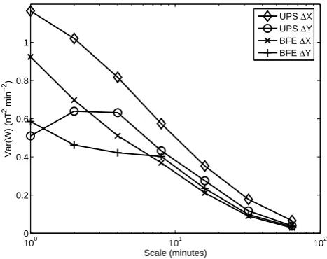
component) and 1Y (east-west component) at both Bror-felde and Uppsala are shown. It is seen that the power is con-centrated to small scales (high frequency). More than 83% of the power is located at the first 4 levels, corresponding to scales smaller thanτ4=24−1=8 min or frequencies higher than 1/32 min−1, and 99% of the power is captured by the details up to level j=J=7. This means that the approx-imation which contains variations with scales longer than 128 min has a very small contribution to the total power in 1X. We also see that the total power is higher for Upp-sala than for Brorfelde, as is expected for a station closer to the auroral oval. However, the spectral distributions of1X and1Y are quite different. For 1X the power decreases monotonically with increasing scale (decreasing frequency), whereas1Y shows a more flat distribution for the first 4 lev-els. Clearly, the dynamics in the two directions are different. A consequence of the localisation of power at high fre-quencies is that temporal averaging of 1X will remove most of the variance in the signal. Thus, it is not so useful to study temporal averages of 1X. It is also worth noting that a T-minute average of 1X will cancel all terms except the endpoints, so that it becomes equiva-lent to estimating the derivative using only two points, i.e. h1Xi_T(t )=1/T (X(t+T )−X(t )).

Returning to the wavelet coefficientsWj,twe see that they representJ different time series that describe variations at different scales, or frequency bands. We may form a set of new time series representing the variance overT minute time windows

v_j2(t )= 1 T

t+T

X

t0_=t

W_j,t2 0, (9)

where we setT=10-min. The power conservation does not strictly hold over 10 min windows but the correlation is still high. Models could now be developed that predict the vari-ancev2_j in X and Y, and thereby estimate not only the mag-nitude of the variation in1Xand1Y, but also at what fre-quencies the disturbances are located. Currently, a study is performed that aims at modifying existing GIC models to make use of this kind of data to calculate the RMS GIC based on power grid data.2However, in this work we will, as a first approximation, assume that the power distribution is constant over time. From Eq. (6) we can define the fractional power as

αj =

ν_j2 1/NP

t1X2t

, (10)

whereP

αj≈1 as the last term approximation of Eq. (6) is close to zero. Next, we form 10-min mean-square (MS)1X as

r2(t )= 1 10

t+9

X

t0_=t

1X(t0)2. (11)

2_{Private communications: R. Pirjola, A. Pulkkinen, A. Viljanen,}

2004

100 101 102

0 0.2 0.4 0.6 0.8 1

Scale (minutes)

Var(W) (nT

2 min

−2

)

UPS ∆X UPS ∆Y BFE ∆X BFE ∆Y

Fig. 1. The figure shows the power distribution of1X and1Y

at Brorfelde (BFE), Denmark, and Uppsala (UPS), Sweden, based

on 525 600 one-minute data points from 1998. 1Xand 1Y are

the one-minute time differences of the north-south and east-west magnetic field components, respectively.

From Eq. (6) we see that r2(t )≈X

j

v2_j(t ), (12)

and with the assumption of a constant power distribution we obtain

v_j2(t )≈αjr2(t ). (13)

To summarise, we may develop a model that predicts the 10 min MS, or RMS, 1X and 1Y. Then, assuming that the power distribution is constant over time we also obtain an estimate of the power at different frequencies. Before we proceed with the solar wind – (1X,1Y) models we study the correlation between MS (1X,1Y) and MS GIC for a single site in Southern Sweden.

3 Correlation between MS1Xand1Y, and MS GIC

The GIC flowing between the transformer neutral and the ground has been measured at a location in Southern Swe-den. The measurements have been carried out for a number of periods during the years 1998 to 2000 and the data set con-sists of almost 100 000 one-minute samples. The measured GIC ranges from−269 Amperes (A) to 195 A. As previously stated, with knowledge about the power grid configuration and the ground conductivity, the GIC may be computed from the time derivative of the horizontal magnetic field (Viljanen et al., 2003). Therefore, we expect to find a correlation be-tween the MS1Xand1Y(r2), and the MS GIC (g2). Using a least-squares fit betweenr2andg2we find

ˆ

100 102 100

101 102

RMS GIC (A)

Linear model (A)

24/09/1998 25/09/1998 26/09/1998 100

101 102

Date

RMS GIC (A)

Observed

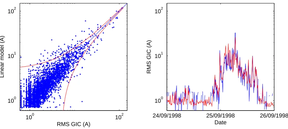
Fig. 2. The left plot in the figure shows the correlation between the 10-min RMS GIC from the linear model and the measured 10-min RMS

GIC. The two curves mark the±5 Amp. error. The right plot shows an example of a GIC event for the period 24 and 25 September 1998.

The blue curve is the observed GIC and the red curve is the GIC from the linear model.

where r1=RMS(1XBF E), r2=RMS(1YBF E), r3=RMS(1XU P S), and r4=RMS(1YU P S). The corre-lation between g2 and gˆ2 is 0.929±0.015 at the 95% confidence level, taking into account the autocorrelation in the time series (see next section). In Fig. 2 the RMS GIC from the linear model is shown together with the measured RMS GIC. The high correlation of the single site empirical linear model indicates that it should be possible to compute the RMS GIC at other locations and for other power grid configurations using the RMS1Xand1Y as inputs.

4 Coupling of the solar wind to RMS1Xand1Y

Now we turn to the solar wind – RMS (1X,1Y) models. We will use a recurrent neural network similar to that described in Lundstedt et al. (2002). This kind of model captures the dynamics in the system that shall be modelled through inter-nal feedback connections. One advantage of using a recur-rent model over a model with time delays on the inputs is that the memory of the system need not be given explicitly. An interesting feature of the recurrent network is that it is possible to rewrite the network equation into a set of coupled differential equations that can be used for further physical interpretation.

The input to the model is the solar wind data from the ACE SWEPAM and MAG instruments (McComas et al., 1998). The 64-s plasma data and the 16-s magnetic field data are resampled to 10-min averages. In addition, the 10-min stan-dard deviations are also used, as the average does not always give a good representation of the original data. For example, two different 10-min intervals may have a similar average proton number density, but very different standard deviations caused by the presence of large variations around the average

due to strong shocks, waves, or turbulence. The input data is collected into the vector

x(t )=µBz(t ), σBz(t ), µn(t ), σn(t ), µV(t ), σV(t ),

(15) whereµ•is the average andσ•is the standard deviation of the solar wind magnetic fieldBz, proton number densityn (hereafter called density), and velocityV. In order to also model any seasonal and local time variation, the sine and co-sine of the fractional year and fractional local time are given at the input

y(t )=

sin2πD 365,cos

2πD 365 ,sin

2πL 24 ,cos

2πL 24

, (16) where D is the decimal day of the year and L is the local time in decimal hours. In total there are 10 inputs.

The output from the model is the predicted logr(t+τ ), whereτ is the prediction horizon. Typically, the time it will take a structure in the solar wind at L1 to reach the Earth’s magnetopause will vary from 30 min (800 km/s) to 80 min (300 km/s). This variable prediction horizon could, in prin-ciple, be handled by either shifting the solar wind input or adjusting τ with a time lag determined by the current so-lar wind velocity. However, this will alter the shape of the time series and artificially modify the dynamics of the sys-tem. Therefore, we setτ=30 min and let the neural network adjust to the given situation.

develop a model that predictsyfromxwith some lead time τ we havey(tˆ +τ )=f (x(t )), whereyˆ is the prediction ofy. This leads to the discrete model

ˆ

yi+k =f (xi), (17)

whereτ=k1t. Now assume that the current time ist0. The latest available input isx−1 and it has been collected over the time interval[t−1, t0]. With a forecast time of τ=k1t we will therefore forecastyk−1, resulting in a true forecast time ofτ0=τ−1t. In order for the model to perform actual forecasts we must have1t≤τ.

The solar wind data and ground magnetic field data are extracted from the six year period 1998–2003, giving in total about 300 000 10-min data samples. However, the complete data set is dominated by quiet conditions withrclose to zero. If the network was to be trained on this set, it would become heavily biased towards predicting quiet levels and thereby poorly predict storm levels. The optimal situation is to have a balanced data set in which all levels of disturbance occur in equal numbers. However, the optimal situation can usually not be achieved due to the distribution of data, and for recur-rent networks the data must also be contiguous. Therefore, a subset is selected using the following algorithm. First, all contiguous sequences longer than 48 h that contain at least one event withr>10 nT/min are selected. This results in 101 sequences with lengths ranging from 48 h up to 120 h that contain both quiet and disturbed conditions. Finally, the se-quences are sorted with respect to the variance inr, and three independent data sets are created by selecting every third se-quence. This results in about 15 000 data points in each set, where each set has a similar mean and standard deviation. The three sets are used for training, validation, and testing. The training set is used for the weight adjustment, the vali-dation set is used to determine the optimal network, and the test set is used to test the network. The input data are nor-malized to cover approximately the range±1 and the output is log-normalized. The neural network can be summarized as

logri(t+τ )=fi(x(t )), (18) where logri is the output and τ is the prediction hori-zon. The goal of the training procedure is to change the free parameters (weights) of f so that the squared error (logri(t )−logri(t ))2 is minimized. The network function f contains input units, hidden units, context units, and an output unit. The units are connected with weights, and each hidden unit and output unit has a bias. The context units con-tain a delayed copy of the hidden units that are fed back into the hidden units; this is the recurrent layer. To a first approx-imation, the recurrent layer is an exponential trace memory, where the weights represent the decay terms. Thus, the con-text units contain the memory of the system.

The weights are initialised to small random values and then the network is trained. Typically, both the training set error and the validation set error decrease during the first part of the training phase as the network adjusts to general

features in the data. Then, as training continues the training error still decreases, while the validation error may occasion-ally increase, passing through several local minima. Finoccasion-ally, the validation error just continues to grow while the training error still decreases. The values of the weights at which the network reached the deepest validation minimum are con-sidered to be the optimal weight. During the first phase the network adjusts to general features in the data, then it picks out more detailed features but also starts to adjust to the noise in the data, and then finally the network continues to adjust to the remaining noise. By monitoring the progress of the validation set error, we can thus find the optimal network.

A large number of networks with different architectures are trained to predict logri, and the optimal network is de-termined using the validation set. The initial network is fully connected and has 10 inputs,nh hidden units,nc=nh context units, and one output. As the output unit and each hidden unit also has a bias, the total number of weights is n=10nh+nh+ncnh+nh+1=1+12nh+n2_h. The number of hidden units is varied overnh=2,3,4,5,6, giving networks withn=29,46,65,86,109 weights.

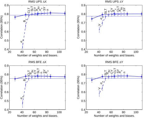
Starting with the model for the RMS1Xat Uppsala we see that the maximum correlation is obtained for a network withnh=5 hidden units (Fig. 3, upper left plot). The confi-dence limits are shown at the 95% level. In computing the correlation and confidence limits we use all three data sets: training set, validation set, and test set. There are almost 40 000 data points but the autocorrelation in both the ob-served series and the predicted series do not fall off to zero quickly. Therefore, the effective number of independent ob-servations (Quenouille, 1952; von Storch and Zwiers, 1999) is reduced by a factor of about 35, giving slightly more than 1000 independent points. In Fig. 3 the horizontal line indi-cates the level at which the correlation is significantly lower than the highest correlation. This means that all models with a correlation above the line perform equally well, but any model falling below the line performs significantly poorer. Thus, it can be seen that there is a significant increase in the correlation going from 2 hidden units to 3 hidden units, and increasing the number of hidden units has very little (or no) effect. Similar results are obtained for UPS1Y, and BFE 1Xand1Y.

20 40 60 80 100 0.4

0.5 0.6 0.7 0.8 0.9

n

SY

σ v σ Bz

CY

SLT

CLT

B z

σ n

Number of weights and biases.

Correlation (95%)

RMS UPS ∆X

20 40 60 80 100

0.4 0.5 0.6 0.7 0.8 0.9

SY

σ Bz

CLT

σ v

CY

n

SLT

σ n

V

Number of weights and biases.

Correlation (95%)

RMS UPS ∆Y

20 40 60 80 100

0.4 0.5 0.6 0.7 0.8 0.9

σ v

SY

n

SLT

CY

σ Bz

CLT

B z

σ n

Number of weights and biases.

Correlation (95%)

RMS BFE ∆X

20 40 60 80 100

0.4 0.5 0.6 0.7 0.8 0.9

n

σ v

SY

CLT

CY

σ Bz

SLT

σ n

V

Number of weights and biases.

Correlation (95%)

RMS BFE ∆Y

Fig. 3. The figure shows the correlation coefficientsC(logr,logr)for networks with different numbers of weights and biases. The plots

show the results for the models, predicting the 10-min root-mean-square (RMS)1X(RMS UPS1X) and RMS1Y (RMS UPS1Y) at

Uppsala, and RMS1X(RMS BFE1X) and1Y (RMS BFE1Y) at Brorfelde. The error bars indicate the 95% confidence levels. The

horizontal line in each plot indicates the level at which the correlation is significantly lower than the highest correlation. The solid curve connected with diamonds corresponds to the fully connected networks with 2, 3, 4, 5 and 6 hidden units. The labels along the dashed curve

show which input that has been removed. The labels have the following meaning: solar wind magnetic field z-component (Bz), proton

number density (n), and velocity (V); standard deviations ofBz(σBz), n (σn), and V (σV); sine (SY) and cosine (CY) of the year; sine (SLT)

and cosine (CLT) of local time.

time we will have a set of 10 different models, each having 9 inputs. The model with the highest correlation is chosen from the set to be used for continued pruning. The process is repeated until there is only one input unit left. The net-work pruning results in the change in correlation according to the points connected with dashed lines in Fig. 3. Each la-bel indicates which input has been removed. The procedure is repeated for Uppsala1Y, and Brorfelde1Xand1Y. For all models the following inputs have no influence: sine and cosine of the year, standard deviations ofBzand velocityV, and densityn. Then there are some differences between the models. In both Uppsala and Brorfelde the1X-models show a weak dependence on the cosine local time (CLT). Looking at the local time distribution of1Xit follows a cosine

11/04/01 12/04/01 13/04/01 10−1

100 101 102

UPS

∆

X (nT/min)

11/04/01 12/04/01 13/04/01 10−1

100 101 102

UPS

∆

Y (nT/min)

11/04/01 12/04/01 13/04/01 10−1

100 101 102

BFE

∆

X (nT/min)

11/04/01 12/04/01 13/04/01 10−1

100 101 102

BFE

∆

Y (nT/min)

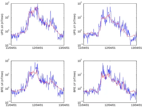
Fig. 4. The four plots show the observed (blue) and predicted (red) 10-min RMS1Xand1Yat Uppsala (UPS) and Brorfelde (BFE) during

a storm in 11–12 April 2001. The correlation in this case is around 0.90. The event was selected from the test set.

related to pressure variations in the solar wind that compress the dayside magnetopause. This is also consistent with the local time variation seen in1X. On the other hand, for1Y the two most important parameters areBzandV that may be interpreted to be more linked to the reconnection process at the magnetopause which causes sub-storms and storms.

As previously mentioned, the prediction lead time is 30 min. We may examine if it is possible to increase the lead time without degrading the performance of the model. We increase the lead time in steps, with continued training of the network, and compute the correlation. It turns out that the correlation for both1Xand1Y monotonically de-creases, even though we may extend the lead time to 70– 90 min before it becomes significantly poorer. However, the 1X-model shows a steeper decrease in correlation than the 1Y-model. This is consistent with the finding above, that solar wind pressure variations are more important for1X than1Y, and that the substorm process dominates the1Y variations. The magnetopause current responds directly to solar wind pressure changes, so the only available lead time is the travel time from L1 to the Earth’s magnetopause. On the other hand, there are additional time delays before the substorm develops after the southward turning ofBz.

5 Discussion

As also shown by Weigel et al. (2002), we found no cou-pling from solar wind densitynto RMS1X. In solar wind coupling studies the density usually enters into the equations through the dynamic pressurep=mnV2, either as the square root ofp or as a linear function ofp (Baker, 1986). If we assume that the geomagnetic fieldXis proportional top, we have

X∝p∝nV2. (19)

Differentiating with respect to timetwe obtain dX

dt ∝ dn

dtV

2_+2nVdV

dt . (20)

Analysing ACE data from 1998 we find that the first term in the above equation completely dominates, leaving us with an equation that does not containn. In addition,dn/dtis related toσnand from the neural network we also find a dependence onσn.

0.63 for the logarithm of the 10-min RMS data. Transform-ing the data to 10-min RMS values the correlation drops to 0.71 and the PE to 0.50. It is difficult to make a comparison with the Weigel et al. (2002) models, as they predict the 30-min average of the absolute value|1X|at higher latitudes. However, forming 30-min RMS the correlation reaches 0.77 and the PE 0.58.

Another issue is that the variance in RMS1X is much larger than the variance in |1X|. The variance of the one-minute1X at Uppsala for 1998 isσ2(1X)=4.23 and the variance of the 10-min RMS 1X is 82% of that, or σ2(RMS1X)=3.45. The 10-min average|1X|(µ(|1X|)) has a variance of only σ2(µ(|1X|))=2.30 which corre-sponds to 55% of the original signal.

We may now look at an example of a prediction. The event is chosen from the test set and extends over two days in April 2001. The four plots in Fig. 4 show the observed RMS1X and1Y in blue and the predicted in red for Up-psala1X(upper left), Uppsala1Y (upper right), Brorfelde 1X(lower left), and Brorfelde1Y (lower right). The units are in nT/min. For both locations, and both directions, the RMS values increase from about 0.5 nT/min to 20 nT/min and with individual peaks close to 100 nT/min. The evolu-tion of the four time series are quite similar, but there are also some smaller differences. We see from the plots that the models predicts the general features well but not the sample to sample variations.

The models have been implemented for real time opera-tion and can be found at the web page http://www.lund.irf.se/ gicpilot/gicforecastprototype. The forecasts are updated ev-ery 10 min and produces a plot of the RMS1Xand1Y for Uppsala and Brorfelde. The linear model given by Eq. (14) has also been implemented to produce RMS GIC forecasts.

6 Conclusions

The main purpose of this work was to develop a model that is capable of forecastingdX/dt anddY /dt in Southern Swe-den. Two magnetic observatories lying at the southwest (Brorfelde) and northeast (Uppsala) corners of the area un-der consiun-deration were selected. The distance between the two sites is about 600 km. At this stage we do not try to pre-dict the one minute1Xor1Y as the time series are domi-nated by fluctuations that are not directly coupled to the solar wind. Instead, we found that using the mean-square (MS) or root-mean-square (RMS) of1Xand1Yformed over 10 min captures a large fraction of the variance in the signal.

Analysing the importance of the input parameters it was found that there was a weak dependence on local time and that the solar wind magnetic fieldBz, velocity V, and stan-dard deviationσnof the density were the most important. It was also found that there might be a slight difference in the solar wind–1Xcoupling compared to the1Ycoupling. The former shows a stronger coupling toσnandV, while the lat-ter has a stronger coupling toBzandV.

From measured GIC at a single location we found that the 10-min RMS GIC can be quite accurately estimated from RMS1Xand1Y from two nearby magnetic observatories. Therefore, we believe that it should be possible to use fore-casted RMS1X and1Y as a general indicator of the GIC level.

In future work the models should be developed to directly predict the variancev2_j(t )at different levelsj. It also has to be seen whether this will significantly improve the estimates of the variation in1Xand1Y and thereby also give further insight into the solar wind–magnetosphere coupling.

Acknowledgements. The author is grateful to the IMAGE network

and the Danish Meteorological Institute for providing the magne-tometer data. The ACE team is acknowledged for providing the solar wind plasma (SWEPAM) and magnetic field (MAG) data. Elforsk AB is acknowledged for providing the GIC data.

This work has been partly funded by the ESA/ESTEC Contract No. 16953/02/NL/LvH and the Swedish National Space Board.

Topical Editor R. Forsyth thanks H. Fichtner and another referee for their help in evaluating this paper.

References

Addison, P. S.: The Illustrated Wavelet Transform Handbook, In-stitute of Physics Publishing, 2002.

Baker, D. N.: Statistical analyses in the study of solar wind-magnetosphere coupling, Solar Wind-Magnetosphere Coupling, 17–38, 1986.

Baumjohann, W. and Haerendel, G.: Entry and dissipation of en-ergy in the Earth’s magnetosphere, in Space Astronomy and So-lar System Exploration: Proceeding of summer school held at

aplbach, Austria, 29 July−8 August, 1986, 121–130, ESA, 1987.

Boberg, F., Wintoft, P., and Lundstedt, H.: Real timeKp

predic-tions from solar wind data using neural networks, Physics and Chemistry of the Earth, 25, 275–280, 2000.

Boteler, D.: Assessment of geomagnetic hazards to power systems in Canada, Natural Hazards, 23, 101–120, 2001.

Boteler, D. H., Pirjola, R. J., and Nevanlinna, H.: The effects of ge-omagnetic disturbances on electrical systems at the Earth’s sur-face, Adv. Space Res., 22, 17–27, 1998.

Cornish, C. R., Percival, D. B., and Bretherton, C. S.: The WMTSA Wavelet Toolkit for Data Analysis in the Geosciences, 84, fall Meet. Suppl., Abstract NG11A-0173, 2003.

Detman, T. R. and Vassiliadis, D.: Review of techniques for mag-netic storm forecasting, 253–266, AGU, 1997.

Gleisner, H. and Lundstedt, H.: Auroral electrojet predictions with dynamic neural networks, J. Geophys. Res., 106, 24 541–24 550, 2001a.

Gleisner, H. and Lundstedt, H.: Neural network-based local model for prediction of geomagnetic disturbances, J. Geophys. Res., 106, 8425–8433, 2001b.

Gonzalez, W. D., Joselyn, J. A., Kamide, Y., Kroehl, H. W., Ros-toker, G., Tsurutani, B. T., and Vasyliunas, V. M.: What is a geomagnetic storm?, J. Geophys. Res., 99, 5771–5792, 1994. Le Cun, Y., Denker, J., and Solla, S.: Optimal brain damage, in

Lundstedt, H., Gleisner, H., and Wintoft, P.: Operational forecasts

of the geomagneticDstindex, Geophys. Res. Let., 29, 34–1–34–

4, 2002.

McComas, D. J., Bame, S. J., Barker, P., Feldman, W. C., Phillips, J. L., Riley, P., and Griffee, J. W.: Solar wind electron proton alpha monitor (SWEPAM) for the Advanced Composition Ex-plorer, Space Sci. Rev., 86, 563–612, 1998.

Nishida, A.: Geomagnetic Diagnosis of the Magnetosphere, 9 of Phys. Chem. Space, Springer-Verlag, 1978.

Percival, D. B. and Walden, A. T.: Wavelet methods for time series analysis, Cambridge University Press, 2002.

Pirjola, R.: Review on the calculation of surface electric and mag-netic fields and of geomagmag-netically induced currents in ground-based technological systems, Surv. Geoph., 23, 71–90, 2002. Quenouille, M. H.: Assoicated measurements, Butterworths

Scien-tific Publications, 1952.

Stone, E. C., Frandsen, A. M., Mewaldt, R. A., Christian, E. R., Margolies, D., Ormes, J. F., and Snow, F.: The Advanced Com-position Explorer, Space Sci. Rev., 86, 1, 1998.

Vassiliadis, D. and Klimas, A. J.: TheDstgeomagnetic response

as a function of storm phase and amplitude and the solar wind electric field, J. Geophys. Res., 104, 24 957–24 976, 1999. Viljanen, A., Pulkkinen, A., Amm, O., Pirjola, R., Korja, T., and

BEAR Working Group: Fast computation of the geoelctric field using the method of elementary current systems and planar Earth models, Ann. Geophys., 22, 101–113, 2004,

SRef-ID: 1432-0576/ag/2004-22-101.

von Storch, H. and Zwiers, F. W.: Statistical analysis in climate research, Cambridge University Press, 1999.