Volume 19 - Article 49 | Pages 1727–1748

(1)

in the population sciences published by the Max Planck Institute for Demographic Research Konrad-Zuse Str. 1, D-18057 Rostock·GERMANY www.demographic-research.org

DEMOGRAPHIC RESEARCH

VOLUME 19, ARTICLE 49, PAGES 1727-1748

PUBLISHED 26 SEPTEMBER 2008

http://www.demographic-research.org/Volumes/Vol19/49/ DOI: 10.4054/DemRes.2008.19.49

Research Article

A transition-based approach to

measuring inequality

Robert Schoen

Claudia Nau

c

°2008 Schoen & Nau.

(2)

1 Introduction 1728

2 Transition measures and their associated population distributions 1729

3 Specifying the projection matrix 1730

4 An illustration involving income inequality 1731

5 Mortality trends and differentials 1732

6 Mortality data and methods 1733

7 Results of the mortality analyses 1735

8 Summary and conclusions 1742

9 Acknowledgments 1743

References 1744

(3)

A transition-based approach to measuring inequality

Robert Schoen1

Claudia Nau2

Abstract

The measurement of inequality is often made using observed population-based distri-butions, such as the distribution of income or the distribution of members of different groups across neighborhoods. Unfortunately, such population distributions confound past and present behavior. Here, we advocate measuring inequality using behavior as reflected by transitions between categories of interest (e.g. income categories) over a specified time period, and show how such measures may be obtained from frequently available data. An illustrative example is provided for the case of income inequality.

The approach is then applied to analyze trends in inequality between men and women in the distribution of ages at death. Observed death distributions indicate that, since 1970, mortality in 4 Western countries experienced increases in inequality that recently leveled off. In contrast, life table death distributions, which solely reflect the implications of a given year’s mortality rates, reveal a peak in inequality followed (in 3 of the 4 countries) by appreciable declines. The results are insensitive to whether inequality is measured by entropy, the Gini Index, or the Index of Dissimilarity. However, the type of population distribution analyzed—whether observed or inferred from the transitions—does make a significant difference in the results obtained. Because distributions derived from transi-tions reflect the inequality implicatransi-tions of behavior over a specified time interval, they are recommended for greater use in analyses of inequality.

1_{Department of Sociology, Pennsylvania State University, University Park PA 16802, USA. E-mail:}

[email protected].

2_{Department of Sociology, Pennsylvania State University, University Park PA 16802, USA. E-mail:}

(4)

1. Introduction

Social inequalities are important indicators of social stratification, social cohesion, and individual well-being. As a result, ways to measure the extent of inequality in a population have received a great deal of methodological attention in the social sciences. Introductions to the large literature on the topic can be found in Cowell (1995), Jenkins (1991), and Sen (1997). A number of different measures, each with its own set of strengths and weaknesses, have been used in a variety of analyses.

For the most part, inequality measures have been based on population distributions observed at a given time with respect to a particular characteristic of interest. For example, measures of income inequality examine how members of different groups are distributed with regard to their level of income, while measures of residential segregation reflect how members of different groups are distributed with regard to place of residence. That approach is straightforward and reasonable, but such population-based measures for a given year (or period) do not reflect behavior at or near that time. Instead, they reflect the complex interplay of current and past behavior that produced the given year’s population distribution. In short, conventional measures do not reflect the inequality implications of behavior at any readily identifiable time period. If the objective of an analysis is to do so, conventional approaches are inappropriate and can produce misleading measures of inequality levels and trends.

This paper provides a way to examine inequality based on transitions during a given period, i.e. on how persons move from one category of the characteristic of interest to another, rather than on the population distributions produced by past and present pat-terns of movement. Such transition rates or proportions reflect behavior during the given period, independent of previous behavior. Those transition values can be used to mea-sure inequality because they imply a unique, long term population distribution. Thus the behavior of a given period can yield a theoretical population distribution that can be used with standard measures of inequality to calculate the inequality implied by behavior during that period.

(5)

2. Transition measures and their associated population distributions

We want to consider behavior over a specific time period, say 1 to 5 years. Let the popu-lation distribution of a given group at the beginning of that interval be described by n-category column vectorxt−1 whosejth element,xj,t−1gives the number of persons in

category j at timet−1. For example, x3,t−1 could denote the number of persons in

income category 3 at timet−1. Analogously, then-category vectorxt, withjth element

xjt, represents the population at timet. The behaviors of interest can, in general, be

re-flected by the elements ofn×npopulation projection matrixAt, which takes the time

t−1population to timet, and hence satisfies the projection relationship

xt=Atxt−1 (1)

Letaijtdenote the element in theith row andjth column ofAt. Elementaijtis essentially

a proportion that represents the fraction of persons in thejth population category at time t−1who are in theith population category at timet. The elements ofAtthus reflect the

results of transitions between categories over time, and describe population behavior over thet−1totinterval.

There are two ways to find the long term (or stable) population distribution implied by At. One is simply to project the initial population far into the future by repeated

applications ofAt. Ultimately, the relative number of persons in the different population

categories will become constant, and those ratios provide the desired population distri-bution (Keyfitz 1977). Alternatively, we can examine the latent (or eigen) structure of At. [To simplify the mathematical presentation, only the basic eigenstructure equations

are given here; for a more complete discussion, see Caswell (2001) or Schoen (2006).] MatrixAt is associated withnroots (or eigenvalues), denoted byλ, which satisfy the

matrix equation

|At−λI|= 0 (2)

where the vertical bars indicate a determinant andIis then×nidentity matrix. With nonnegative elementsaijt,Athas a unique, real, and largest (or dominant) root whenever

Ant(n−2)+2has all positive elements (which is usually the case for the matrices discussed

here). Associated with dominant eigenvalueλtis dominant right eigenvectorut, defined

by

λtut=Atut (3)

The long term distribution of the population implied by At is provided by n-element

right eigenvectorut. It is the only right eigenvector ofAtwhose elements all have real,

nonnegative values. The elements ofutare only specified up to a scaling factor, but their

(6)

Computationally, finding the eigenstructure of a matrix can be quite tedious. In prac-tice, however, mathematical software (e.g. Maple, Mathematica, S+) are readily available. They make finding the roots and eigenvectors of a matrix, and hence the long term popu-lation distribution implied by a given popupopu-lation projection matrix, a rather simple task.

When inequalities in mortality are of interest, as in a later application here, a different way of finding the theoretical population distribution of interest may be preferable. Ob-served age-group-specific death rates (i.e. numbers of deaths for a given group in a given age interval divided by the number of persons in that group in that age interval) may well be available and can be used to calculate a life table (Preston et al. 2001). The life table shows the number of persons in a hypothetical cohort who survive from birth to every age under the given death rates and, via subtraction, gives the number of persons in the cohort dying in every age interval. Those life table cohort deaths can provide an appropriate theoretical distribution.

3. Specifying the projection matrix

Several frequently available sources of data make it possible to create the requisite popu-lation projection matrix for many potential areas of application. The essential requirement is that the data provide each person’s category at the beginning and end of the projection interval. Prospective or panel data can provide contemporaneous information on each individual’s beginning and ending status. Retrospective data can provide information on the previous status of those surviving. [On the assumption of no (or known) differen-tial mortality between categories, survivorship can also be taken into account (Schoen 1988:76-79).] The element in theith row andjth column of the population projection matrix is then given by the ratio of (i) the number of persons in categoryiat the end of the interval who were in categoryjat the beginning of the interval divided by (ii) the total number of persons in categoryjat the beginning of the interval.

The logic of the population projection matrix relates persons in each category of the ending population to their category at the beginning of the interval. Persons who are born or who migrate into the population of interest during the projection interval must be related to an appropriate initial category, but there is generally a reasonable way to do so. Births can usually be given the category of their parents. Persons initially residing outside the area of interest can be related to their end of interval residential category. Persons who initially had no income can be related to a "no income" category. Such behaviorally plausible assignments make it possible to fully specify the values used in the calculation of the elements of the population projection matrix.

(7)

the Markovian assumption that only the current state affects the risk of transfer, with past history irrelevant. Both assumptions are strong and typically violated. Past experiences often affect transfer risks, as do individual characteristics such as length of time in a particular category. Events in a specified time interval may be influenced by features of preceding intervals, which are not considered. Even in short time intervals, the risks of transition may change substantially over time. Investigators need to satisfy themselves that the model is sufficiently realistic for the purposes intended. The choice of categories also embodies judgments about the nature of the behavior being studied. For example, a study of income inequality over time should be based on categories that reflect the income distribution over the entire time span considered.

4. An illustration involving income inequality

The unequal distribution of income across groups is a longstanding focus of inequality research. To provide an illustration of how the transition-based approach can be applied, we examine the inequality between two time periods, 1963-66 and 1966-70. That is directly analogous to comparing the income inequality between men and women, between single persons and married persons, or between any specified pair of groups. We use data examined by Shorrocks (1976), which are shown in the Appendix Table. Those data give, for five income categories, (i) the income distribution of Shorrocks’ 1963 sample (total number of persons = 800), (ii) a transition (projection) matrix showing the distribution of income in 1966 of persons in each income category in 1963, and (iii) a transition matrix showing the distribution of income in 1970 of persons in each income category in 1966. The Appendix Table also shows the estimated sample population by income category in 1966, obtained by projecting the 1963 population to 1966 using the 1963-66 projection matrix, and the estimated 1970 sample population obtained by projecting the 1966 population using the 1966-70 projection matrix. For the conventional approach, we consider the 1966 income distribution as characterizing "Group A", the 1970 income distribution as characterizing "Group B", and assess the inequality between those groups. The projection matrices in Panels B and C of the Appendix Table have theoretical population distributions by income category (i.e. dominant eigenvectors) associated with them. Those theoretical income distributions, scaled to yield a total of 800 persons, are shown in the last two columns of Panel A of the Appendix Table. To apply the transition-based approach, we consider the 1963-66 experience as characterizing Group A, the 1966-70 experience as characterizing Group B, and measure the inequality between the theo-retical distributions implied by those two transition matrices.

(8)

Measure Inequality Based on

Data Populations Theoretical Populations

Gini Index 0.1002 0.2282

Index of Dissimilarity 0.0894 0.2147

For both measures, the inequality based on the theoretical populations is more than twice as large as that based on the sample (data) populations. The result is not surprising, because the composition of data populations generally changes gradually, as it represents a complicated weighted average of past behavior. In contrast, theoretical populations are based solely on the behavior of a specified period. As a result, the transition-based approach reflects the full impact of the differences between the 1963-66 and 1966-70 patterns of transitions.

This illustrative application indicates some noteworthy features of the transition-based approach. First, it readily adapts to any number of categories. If there are n categories of interest, the projection matrix has n rows and n columns. Second, the method imposes no restrictions on movements between states. Persons can move freely, and repeatedly, between the states in the model as they do in the actual population. In addition, as long as the underlying rates do not change, the duration of the period of observation does not influence the theoretical population distribution. A longer duration affects the roots of the projection matrix, but not the eigenvectors that determine the theoretical population of interest.

5. Mortality trends and differentials

To investigate whether the use of observed versus theoretical distributions can make a significant difference in substantive analyses of inequality, we examine the case of sex differentials in mortality. The life table approach, as described above, is used to generate the theoretical distribution of deaths based on the experience of a hypothetical cohort, and three different inequality measures are used so that the effect of using observed ver-sus theoretical death distributions can be clearly distinguished from inequality measure effects.

(9)

1960 which could not be explained by aggregate socioeconomic inequalities. As they noted, that has important policy implications, as it points to the need to reduce inequality in longevity as well as to increase life expectancy.

Goesling and Firebaugh (2004) used data for 169 countries to examine trends in between-country life expectancy between 1980 and 2000. Continuing a trend that began in the first half of the 20th century, inequality in the distribution of life expectancy across countries declined in the 1980s. During the 1990s, however, between-country inequality increased. Changes in mortality differentials by sex were explored by Glei and Horiuchi (2007). Using long term data on life expectancy at birth [e(0)] from 29 high-income countries, they found that the difference between a country’s male and femalee(0)values widened during most of the 1900s. Recently, however, the gender gap in longevity nar-rowed in most countries considered. Here, we seek to further examine trends in mortality sex differentials to see whether they differ when observed deaths are used instead of life table deaths. Rather than using the difference between male and female longevity, we em-ploy three standard measures of inequality. In every population considered, we calculate our measures separately for life table and observed distributions of deaths, to see whether the transition-based life table distributions and the observed population distributions de-pict different trends in inequality. To the best of our knowledge, such a comparison has never previously been made.

6. Mortality data and methods

We use data for four countries: England and Wales 1840-2002, Italy, 1880-2002, Swe-den, 1840-2002, and the United States, 1900-2002. For the first three countries, all data are from the Human Mortality Database. For the United States, life table values for 1900-1998 are from Haines (2006:Tables Ab988-1047), and data on observed deaths are from (i) the U.S. National Center for Health Statistics (NCHS) (2007) for the years 1900 through 1946 and (ii) the Human Mortality Data Base for the years 1947 through 2002.

In all cases, sex-specific death rates and numbers of deaths were determined, by single years of age, for each data year examined. Single years of age were available in the Human Mortality Database. For the United States, linear interpolation was used to obtain single year values from grouped data. The highest age recognized was 104.

(10)

random-ness), and has often been used in mortality analysis (Edwards and Tuljapurkar 2005; Vaupel 1986). Here it is applied following the manner described in White (1986), i.e.

H= (H∗−H)/Hˆ ∗ (4)

The overall life course component is

H∗₌₋X

k

pk lnpk (5)

with the sum overkspanning both gender groups,pkdenoting the proportion of the total

number of deaths that are male (or female), andlnindicating the natural logarithm. The minus sign makes the measure a positive quantity, as the logarithm of a proportion is a negative number. The age-group specific component is

ˆ

H =−X i

[d(i)/`(0)]X

k

[dk(i)/d(i)]ln[dk(i)/d(i)] (6)

where the sum overiranges over all ages, the sum overkspans both gender groups,d(i) indicates the total number of life table [or observed] deaths at agei, anddk(i)indicates

the life table [or observed] number of groupkdeaths at agei. The symbol`(0)denotes the total number of observed deaths or the initial (age 0) size of the life table cohort, including both males and females. In the life table calculations, we assumed the conventional sex ratio at birth (srb) of 105 males per every 100 females (though onlyHis sensitive to the srb used).

The Gini Index is one of the most frequently used measures of inequality, and is a standard measure in studies of income inequality (White 1986). For either gender group k, it can be written as

G=

P i

P

jd(i)d(j)|[dk(i)/d(i)]−[dk(j)/d(j)]|

2`(0)2_[d

k/`(0)] [1−dk/`(0)]

(7)

where the sums overiandj range over all ages, the vertical bars indicate an absolute value, anddk is the total number of deaths in reference gender groupk. The Index of

Dissimilarity is another frequently used measure, and is a standard in studies of residential segregation (White 1986). For gender groupsmandf, it can be written

D= (1/2)X

i

|dm(i)/dm−df(i)/df| (8)

(11)

7. Results of the mortality analyses

Figures 1, 2, and 3 show inequality measuresH, G, andD, respectively, for England and Wales, Italy, Sweden, and the United States for each available year from 1900 to 2002. Similarly, Tables 1, 2, and 3 present those inequality measures for available years ending in the digit "0", beginning in 1840 and adding the most recent year, 2002. In every case, separate calculations were made based on observed deaths and life table deaths. The particularly pronounced spikes in inequality in England and Wales are associated with the 1918 Pandemic and World War II. The latter may also reflect administrative procedures followed in recording wartime deaths (personal communication from Seamus Spark, January 3, 2007). To a lesser extent, a similar war-related phenomenon may have occurred in Italy during 1944 and 1945.

The results indicate that, over most of the 20th century, gender inequality in mortality was increasing in all four countries considered. That is consistent with previous work, and is reflected by all three measures and by both observed and life table death distributions. Since about 1970, however, the trends depicted by observed and life table distributions have diverged.

(12)

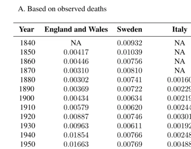
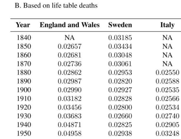
Table 1: Entropy measure (H) values of male/female inequality in mortality in four western countries, 1840-2002

A. Based on observed deaths

Year England and Wales Sweden Italy United States

1840 NA 0.00932 NA NA 1850 0.00417 0.01039 NA NA 1860 0.00446 0.00756 NA NA 1870 0.00310 0.00810 NA NA 1880 0.00302 0.00741 0.00160 NA 1890 0.00369 0.00722 0.00229 NA 1900 0.00434 0.00634 0.00219 0.00277

1910 0.00579 0.00620 0.00244 0.00369 1920 0.00887 0.00746 0.00301 0.00324 1930 0.00963 0.00611 0.00192 0.00332∗

(13)

Table 1: (Continued)

B. Based on life table deaths

1840 NA 0.03185 NA NA 1850 0.02657 0.03434 NA NA 1860 0.02681 0.03048 NA NA 1870 0.02736 0.03061 NA NA 1880 0.02862 0.02953 0.02550 NA 1890 0.02987 0.02820 0.02588 NA 1900 0.02990 0.02927 0.02535 0.02685 1910 0.03182 0.02828 0.02566 0.02854 1920 0.03456 0.02800 0.02534 0.02642 1930 0.03683 0.02660 0.02740 0.02952 1940 0.04871 0.02825 0.02905 0.03525 1950 0.04958 0.02938 0.03248 0.04537 1960 0.06443 0.03743 0.04600 0.05789 1970 0.07250 0.05062 0.05681 0.06949 1980 0.07198 0.06834 0.07442 0.07069 1990 0.06553 0.06666 0.07388 0.06327 2000 0.05337 0.05788 0.06918 0.04953∗∗

2002 0.05002 0.05440 0.06849 NA

(14)

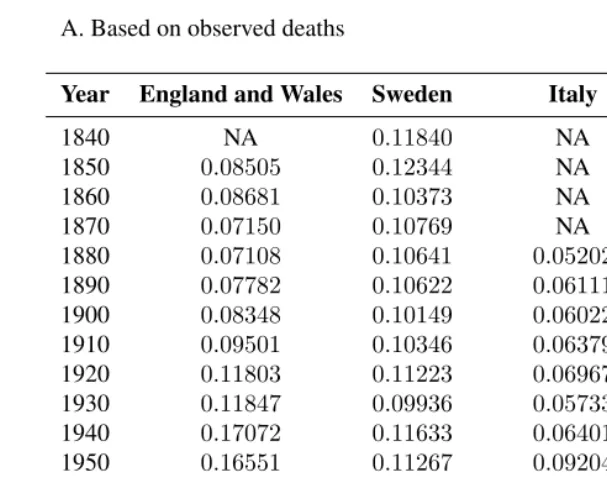
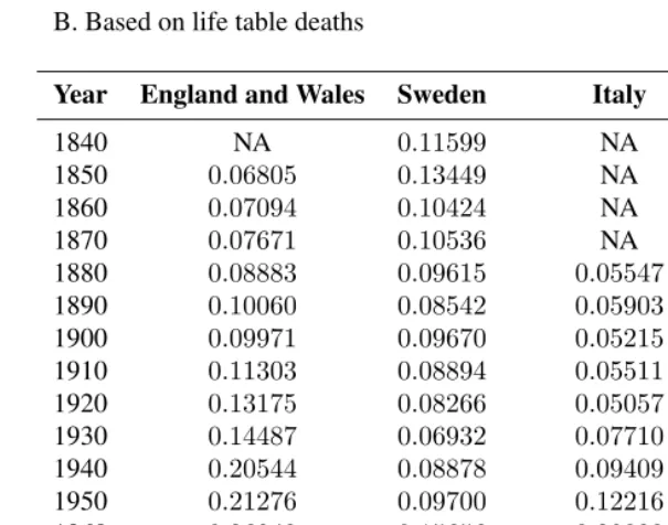
Table 2: Gini index values of male/female inequality in mortality in four western countries, 1840-2002

1840 NA 0.11840 NA NA 1850 0.08505 0.12344 NA NA 1860 0.08681 0.10373 NA NA 1870 0.07150 0.10769 NA NA 1880 0.07108 0.10641 0.05202 NA 1890 0.07782 0.10622 0.06111 NA 1900 0.08348 0.10149 0.06022 0.06544 1910 0.09501 0.10346 0.06379 0.07899 1920 0.11803 0.11223 0.06967 0.07281 1930 0.11847 0.09936 0.05733 0.07179∗

(15)

2002 0.21470 0.23043 0.28515 NA

(16)

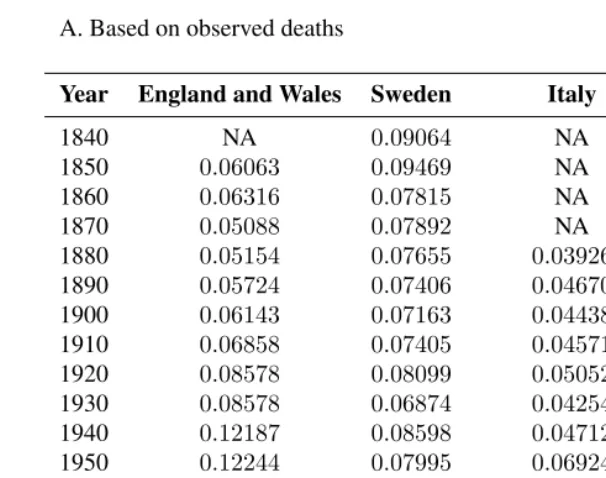
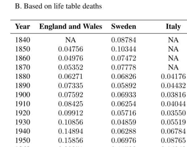
Table 3: Dissimilarity index values of male/female inequality in mortality in four western countries, 1840-2002

1840 NA 0.09064 NA NA 1850 0.06063 0.09469 NA NA 1860 0.06316 0.07815 NA NA 1870 0.05088 0.07892 NA NA 1880 0.05154 0.07655 0.03926 NA 1890 0.05724 0.07406 0.04670 NA 1900 0.06143 0.07163 0.04438 0.04812 1910 0.06858 0.07405 0.04571 0.05506 1920 0.08578 0.08099 0.05052 0.05585 1930 0.08578 0.06874 0.04254 0.05247∗

(17)

2002 0.16122 0.17171 0.21462 NA

(18)

Figure 1: Entropy measure (H) of male/female inequalities in mortality over time in four western countries, 1900-2000

(19)

Figure 2: Gini index of male/female inequalities in mortality over time in four western countries, 1900-2000

(20)

Figure 3: Dissimilarity index of male/female inequalities in mortality over time in four western countries, 1900-2000

Note:Dissimilarity index values for England and Wales in several years are off scale. Those values are (i) for life table deaths: 1916 (0.31706), 1917 (0.3895) and 1918 (0.33861) and (ii) for observed deaths:

(21)

8. Summary and conclusions

The trend in gender inequality in mortality since the 1970s is markedly different when inequality is based on observed death distributions rather than life table death distribu-tions. The life table distributions, which show the implications of the death rates observed in a given year, show a peak in inequality followed by a notable decline. In England and Wales and the United States, a clear peak in the 1970s was followed by a marked decline. Italy showed a small peak in 1991 followed by a small decline. Sweden was intermedi-ate, with a peak in the 1980s followed by a decline of over 20%. Those patterns do not depend on whether inequality is measured by entropy (H), the Gini Index, or the Index of Dissimilarity. They are also consistent with the pattern found by Glei and Horiuchi (2007) based on differences between male and female life expectancy at birth.

Recent trends in inequality in mortality are quite different when based on observed death distributions, which confound current mortality with past demographic behavior. Again the three inequality measures provide the same results—a longer continuation of the increase in inequality followed by a plateau extending to 2002. No decline in inequality was evident in any of the four countries considered. It is difficult to argue that including the effects of past fertility, mortality, and migration improves the measurement of gender inequality in mortality in any given year. The use of observed death distribu-tions thus disguises recent trends in inequality.

Much of the literature on inequality, including most studies of income inequality and residential segregation, use data analogous to the observed death distributions. There is thus a real possibility that reported trends in inequality may be compromised by the use of data that confounds current and past behavior. The illustrative example on income inequality in Section 4 reinforces that view. The transition-based approach described here, which uses longitudinal or retrospective data to produce time-specific behavioral measures, is therefore recommended as a feasible method for measuring the inequality implications of behavior observed during a specified period of time.

9. Acknowledgments

(22)

References

Caswell, H. (2001). Matrix population models: Construction, analysis, and interpreta-tion. Sunderland: Sinauer, second ediinterpreta-tion.

Cowell, F. A. (1995). Measuring Inequality. London: Prentice Hall/Harvester Wheat-sheaf, second edition.

Edwards, R. D. and Tuljapurkar, S. (2005). Inequality in life spans and a new perspective on mortality convergence across industrial countries. Population and Development Review31(4): 645–674.

Glei, D. A. and Horiuchi, S. (2007). The narrowing sex differential in life expectancy in high-income populations: Effects of differences in the age pattern of mortality. Popu-lation Studies61(2): 141–159.

Goesling, B. and Firebaugh, G. (2004). The trend in international health inequality. Popu-lation and Development Review30(1): 131–146.

Haines, M. (2006). Death rates by sex and age: 1900-1998. In: Carter, S. B., Gartner, S. S., Haines, M. R., Olmstead, A. L., Sutch, R., and Wright, G. (eds.).Historical statistics of the United States: Earliest times to the present. New York: Cambridge University Press: Ab912-Ab1137, millennial edition.

Human Mortality Database (2006). [electronic resource]. Berkeley and Rostock: Univer-sity of California and Max Planck Institute for Demographic Research. Downloaded October 2006 from www.mortality.org.

Jenkins, S. (1991). The measurement of income inequality. In: Osberg, L. (ed.).Economic inequality and poverty: International perspectives, pp. 3–38. Armonk: Sharpe. Keyfitz, N. (1977). Introduction to the mathematics of population. Addison-Wesley,

second edition. Reading: Addison-Wesley.

Preston, S. H., Heuveline, P., and Guillot, M. (2001). Demography: Measuring and modeling population processes. Oxford: Blackwell.

Schoen, R. (1988).Modeling multigroup populations. New York: Plenum Press. Schoen, R. (2006).Dynamic population models. Dordrecht: Springer.

Sen, A. (1997).On economic inequality. Oxford: Clarendon Press.

(23)

Shorrocks, A. F. (1976). Income mobility and the Markov assumption. The Economic Journal86(343): 566–578.

U.S. National Center for Health Statistics (2007). Historical vital statistics of the United States. [electronic resource]. Hyattsville: U.S. Department of Health and Human Services. Downloaded January 2007 from www.cdc.gov/nchs/products/pubs/pubd/vsus/historical/historical.htm.

Vaupel, J. W. (1986). How change in age-specific mortality affects life expectancy. Popu-lation Studies40(1): 147–157.

White, M. J. (1986). Segregation and diversity measures in population distribution. Popu-lation Index52(2): 198–221.

(24)