Theoretical Approaches to the Characterization of Water, Aqueous Interfaces, and Improved Sampling of Protein Conformational Changes

(1)

University of New Orleans University of New Orleans

ScholarWorks@UNO

University of New Orleans Theses and

Dissertations Dissertations and Theses

Summer 8-2-2012

Theoretical Approaches to the Characterization of Water,

Aqueous Interfaces, and Improved Sampling of Protein

Conformational Changes

Alexis J. Lee

UNIVERSITY OF NEW ORLEANS, [email protected]

Follow this and additional works at: https://scholarworks.uno.edu/td

Part of the Physical Chemistry Commons, and the Theory and Algorithms Commons

Recommended Citation Recommended Citation

Lee, Alexis J., "Theoretical Approaches to the Characterization of Water, Aqueous Interfaces, and Improved Sampling of Protein Conformational Changes" (2012). University of New Orleans Theses and Dissertations. 1511.

https://scholarworks.uno.edu/td/1511

This Dissertation is protected by copyright and/or related rights. It has been brought to you by ScholarWorks@UNO with permission from the rights-holder(s). You are free to use this Dissertation in any way that is permitted by the copyright and related rights legislation that applies to your use. For other uses you need to obtain permission from the rights-holder(s) directly, unless additional rights are indicated by a Creative Commons license in the record and/ or on the work itself.

(2)

Theoretical Approaches to the Characterization of Water, Aqueous Interfaces, and Improved Sampling of Protein Conformational Changes

A Dissertation

Submitted to the Graduate Faculty of the University of New Orleans

in partial fulfillment of the requirments for the degree of

Doctor of Philosophy in

Chemistry

by

Alexis J. Lee

B.S. University of Louisiana, Lafayette, 2006

(3)

c

(4)

(5)

Acknowledgments

When I consider all the people to whom I owe thanks for getting me to this point in my life and education, quite a lengthy list compounds. First and foremost, I offer my sincerest gratitude to my advisor, Professor Steve W. Rick, who has guided me in so many ways throughout my graduate career. Imparting his knowledge, wisdom, and time are things for which I am eternally grateful. I could not have asked for a more understanding and patient advisor. I very much appreciate my committee, Professor David Mobley, Professor Chris Summa, and Professor Edwin Stevens, for their time and input. Thanks are owed to the University of New Orleans Department of Chemistry for five wonderful years.

My dear friend and former lab mate, Dr. Hongtao Yu, deserves special acknowl-edgement. He helped me so much in learning Fortran, in classes, and taught me about Chinese culture. My current lab mates, Marielle Soniat, Kalika Murthy Aritakula, Dr. Sreeja Parameswaran, I just adore. Thank you for being so friendly and making my last few years so joyous.

(6)

List of Figures

1.1 Aggregation of partial positive charge (blue) at the air/water interface with a negatively-charged (red) layer beneath the surface; charges disperse into the bulk, averaging to neutrality. . . 4

3.1 The oxygen-oxygen pair correlation function for the TIP4P+DCT and TIP4P-FQ+DCT potentials (dashed lines) and X-ray experimental data (solid line).[1] The correlation function for the TIP4P+DCT model has been shifted by 2 units. 23 3.2 Density of (a) TIP4P+DCT (circles), TIP4P/2005[2](crosses), and

Ew[3](triangles) and (b) FQ+DCT (circles and dashed line) and TIP4P-FQ[4] (diamonds) compared to Experiment[5](solid line). . . 26 3.3 Probability distribution of the difference in the number of hydrogen bonds a

molecule forms as a donor and as an acceptor at three different temperatures, 273 K (dashed line), 298 K (solid line), and 373 K (dotted line) . . . 28

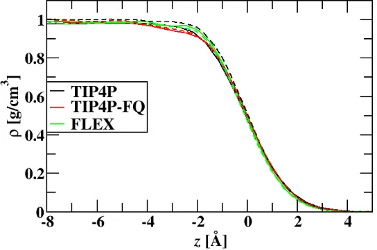
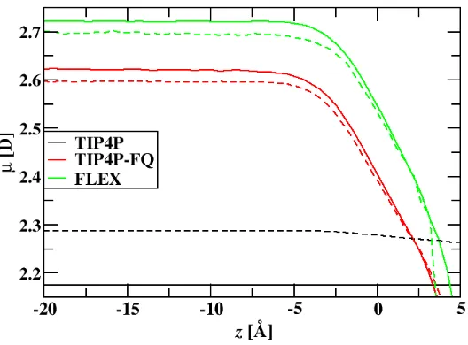
4.1 Average water density profile across the air/water interface as a function of z for the different water models investigated. Dashed lines have intermolecular charge transfer. Solid lines do not. The Gibbs dividing surface is at 0 ˚A. . . . 37 4.2 Profile of the average total dipole of water across the air-water interface for the

different water models investigated. Dashed lines have intermolecular charge transfer. . . 39 4.3 Profile of the average distance between first solvation shell water oxygens

minus the average bulk distance across the air-water interface for the water models investigated. Dashed lines have intermolecular charge transfer. . . 40 4.4 Difference in number of hydrogen bond acceptors and donors as a function of

z for the water models investigated. Dashed lines represent the intermolecular charge transfer models. . . 41 4.5 Molecular charge density profile as a function of z for the charge transfer

models, with an estimate of the charge distribution for the CT-TIP4P water model with an interfacial cross section of 100 nm. . . 41 4.6 Integrated charge as a function of z for the charge transfer models, with the

integrated estimate of the charge distribution for the CT-TIP4P water model with an interfacial cross section of 100 nm. . . 42 4.7 Electrostatic potential as a function of z across the air/water interface. Dashed

lines are charge transfer models. The inset is an enhanced view near the GDS. 43 4.8 Molecular density profile for the ice/liquid interface with TIP4P-FQ+DCT

(9)

4.9 Dipole moment of the ice/liquid interface with TIP4P-FQ+DCT water as a function of z. . . 48 4.10 Molecular charge density profile at the ice/liquid interface with TIP4P-FQ+DCT

water as a function of z. . . 49 4.11 Surface charge at the ice/liquid interface with TIP4P-FQ+DCT water as a

function of z. . . 50

5.1 Scaled energy, Eλ versus time for (A) the alanine dipeptide system with τ= 1 (dotted line), 2 (dashed line), and 20 ps (solid line) and (B) the trpzip2 system with τ=5 (dotted line), 10 (dashed line), and 40 (solid line) ps. The diamonds show the equilibrium values for Eλ. . . 60 5.2 Energy versus time for two replicas of the alanine dipeptide system, with the

T = 300 K (solid line) and the driven replica (TA = 300 K,TB = 420 K, and TM = 350 K) with (A) τ = 1 ps and (B) τ = 20 ps. Vertical lines indicate the points at which exchanges were accepted. . . 62 5.3 Distribution of energy at 298 K for the alanine dipeptide system for 5 replica

REDS2 (solid lines) and 22 replica RE (diamonds) for (A) the total energy and (B) the torsional energy. . . 64 5.4 Distribution of energy at 298 K for the trpzip2 system for 10 replica REDS2

(solid lines) and 16 replica REDS (diamonds) for (A) the total energy and (B) the torsional energy. . . 64 5.5 Average energy as a function of temperature for the alanine dipeptide system

for 5 replica REDS2 (solid lines) and 22 replica RE (diamonds) for (A) the total energy and (B) the torsional energy. . . 65 5.6 Average energy as a function of temperature for the trpzip2 system for 10

replica REDS2 (solid lines) and 16 replica REDS (diamonds) for (A) the total energy and (B) the torsional energy. . . 66 5.7 The population of the C7eq/C5 structure for the alanine dipeptide at T = 298

K for 5 replica REDS2 (lines) and 22 replica RE (symbols). The diamonds and solid line represent the simulation that started in theαR/β2 configuration and the circles and dashed line in the C7eq/C5 structure. . . 66 5.8 The temperature of a selected replica as a function of time for the trpzip2

(10)

List of Tables

3.1 Parameters for the TIP4P-DCT, TIP4P[6], TIP4P/2005[2] and TIP4P-Ew[3] models. . . 22 3.2 Parameters for the TIP4P-FQ+DCT and TIP4P-FQ[7] models. . . 23 3.3 Average values for the magnitude of the total charge, dipole moment and

quadrupole moments of liquid water at a temperature of 298 K and a pressure of 1 atm. . . 24 3.4 Properties of selected water models at T = 298 K and P = 1 atm. density,ρ,

average potential energy per molecule, E, isothermal compressibility,κT, coef-ficient of thermal expansion,αp, constant pressure heat capacity, Cp, dielectric constant,, and translational diffusion constant D, compared to experimental values.[5, 8, 9, 10, 11] . . . 25 3.5 Liquid densities at a pressure of 1 atm, compared to experiment.[5] . . . 26

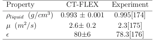
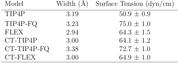
4.1 Comparison of the Properties of Pure Water Between Simulation Results for the CT-FLEX Model and Experiment at 298 K. . . 36 4.2 Interfacial Widths and Surface Tensions for the Models Investigated . . . 38 4.3 Temperature of the ice/water charge transfer simulation and the melting

tem-perature for the model found by Chung and Rick[12]. . . 47

(11)

Abstract

Methods to advance the understanding of water and other aqueous systems are devel-oped. This work falls into three areas: The creation of better interaction potentials for water, the development of superior methods for sampling configurational space, and the applications of these methods to understand systems of interest. Charge transfer has been shown by ab initio methods to be important in the water–water and water–ion interactions. A model for treating charge transfer in liquid water and aqueous systems is presented in this manuscript. The model is called Discrete Charge Transfer (DCT) and is based on the commonly-used TIP4P/2005 model, which represents the charge distribution of water molecules with three charge sites. Such models have been very successful in reproducing many of the physical properties of water. Charge transfer is introduced by transferring a small amount of charge, -0.02 e, from the hydrogen bond acceptor to the hydrogen bond donor, as has been in-dicated by electronic structure calculations. We have parameterized both polarizable and non-polarizable potentials, optimized to include charge transfer. Methods to surmount the obstacles incurred by the introduction of charge transfer, which involve the amount of charge transfer at large distances and implementation into Molecular Dynamics simulation, is pre-sented, along with our results assessing the importance of charge transfer in liquid water and aqueous systems. Also presented is a method for improving efficiency of a sampling technique, Replica Exchange, by reducing the number of replicas. The improved method is called Replica Exchange with Driven Scaling (REDS2).

(12)

Chapter 1 Introduction

Molecular simulation is a powerful tool. The evolution of technologies has led to an

ever-increasing demand for more efficient methods of understanding the microscopic realm.

“Experiments do not always come with explanations,” an apothegm of science, is itself an

adequate impetus to search for more innovative means by which data may be obtained.

Microscopic length- and timescales are now accessible for exploration, due to increased

so-phistication of computers, bridging the microscopic world and the macroscopic realm of the

laboratory. Detailed characterization of structural information and interactions on the

mi-croscopic scale can be costly, difficult, or impossible to obtain by conventional methods.

Simulated experimentation techniques are aimed at gaining understanding of the properties

of molecular systems by methods that can complement or even replace laboratory approaches.

Two classes of computational methods for obtaining valuable molecular information,

the latter of which is of principal concern, are ab initio (quantum principles) calculations

and empirical potential energy models. First principles techniques are purely theoretical, in

that no experimental data is involved in the computation of system properties. Ab initio

cal-culations alone, though extremely robust, are computationally expensive and cannot provide

dynamical information about a system. Fortunately, a cheaper approach exists. Empirical

(13)

are a set of mathematical functions and parameters designed to describe the potential energy

of a system of particles.[13, 14, 15, 16, 17, 18]

Molecular simulations are limited by the accuracy of the potential energy model

which is used. The development of accurate yet computationally efficient models is a

con-stant challenge. Results of molecular simulation can be sensitive to such factors as the

model utilized, how a surface is defined, the definition of a hydrogen bond, and

polariz-ability, leading to qualitatively different results, especially for anions at liquid water/air

interfaces.[19, 20, 21, 22, 23] Molecular simulations can also be affected by the timescale of

the model. Two ways to surmount this issue are to build more efficient potentials or use

faster, more efficient sampling techniques. My research over the last 5 years has focused on

the development of the following:

• DCT (Discrete hydrogen-bond-based Charge Transfer): A new water potential that

treats charge transfer (CT) in hydrogen-bonded and asymmetrically-bonded systems.[24]

• REDS2 (Replica Exchange with Dynamical Scaling): A simulation technique which

improves the efficiency of conventional replica exchange (RE) by reducing the number

of replicas.[25]

The new model, Discrete Charge Transfer[24], or DCT, was parameterized for the

non-polarizable and polarizable potentials, TIP4P[6] and TIP4P-FQ[7], respectively, and

applied to the study of aqueous bulk and interfacial charge transfer.

Aqueous interfaces are often the home of curious chemical processes in nature[26],

including electrochemical reactions associated with aqueous batteries[27], protein solvation

and folding[28, 29] and “on water” organic catalysis.[30, 31, 32] Despite extensive

experimen-tal and theoretical research on interfaces, an accurate depiction of the air/water interface

has yet to be agreed upon by the scientific community. The need for a proper understanding

of the structure and chemistry of the air/water interface is relevant to many fields of study,

(14)

Since the 19th century, scientists have observed a counterintuitive electrokinetic

phe-nomenon that occurs when air bubbles and oil droplets in water are subjected to an external

electric field. The air bubbles and oil droplets exhibit negative electrophoretic mobility,

act-ing as negatively-charged colloidal particles.[34, 35, 36, 37] Numerous explanations have been

proposed as to why the bubbles and droplets drift toward the cathode. Theories put forth

include aggregation of OH− _{at the surface, the existence of a diffuse (or shear) layer of OH}−

just below the surface[38, 39, 40, 41], and dipole ordering of the surface water molecules[42],

none of which offers a satisfactory explanation of all the physical properties observed at the

interface. Spectroscopic data suggest that the first two or three molecular layers near the

interface are populated by hydronium ions, while approximately 10-20 ˚A into the bulk,

hy-droxide ions counterbalance a more positive surface under normal pH conditions. Hyhy-droxide

at the surface would produce opposite behavior.[43, 44, 45, 46, 47, 48, 49, 50, 51, 52]

Recent ab initio molecular dynamics (AIMD) simulations have reported dangling

O–H bonds (non-hydrogen-bonded surface [water] hydrogens) at the liquid/vapor interface,

consistent with surface-specific vibrational sum-frequency generation (SFG) data.[33] Such

asymmetrically-bonded surface water molecules will be discussed later in this text. As

men-tioned previously, spectroscopic and theoretical experiments of small clusters and larger

wa-ter systems predict higher concentration of hydronium ions at the surface.[43, 44, 45] Such

predictions, however, do not explain the electrophoretic mobility of air bubbles toward the

cathode. Understanding the electrokinetic properties of water is the crux of the fundamental

debate over whether the surface of water is acidic or basic.

A 2009 submission to Chemical Physics Letters (CPL) by Richard Saykally[53]

ac-knowledged the intense controversy over the surface structure of water, and consequently,

had an entire issue ofCPLdedicated to this dispute. The July 2010 issue ofC&EN Magazine

featured the tumultuous debate in an article aptly titled, “Storm in a Teacup,” where

sci-entists from both camps–Waters surface: Acidic or Basic?–presented justifications for their

(15)

sug-Figure 1.1: Aggregation of partial positive charge (blue) at the air/water interface with a negatively-charged (red) layer beneath the surface; charges disperse into the bulk, averaging to neutrality.

gesting that charge transfer (CT) between neighboring water molecules at the air/water

interface may have an effect on the total interfacial charge, giving rise to a response to an

external/applied electric field [55], as in Figure 1.1.

We assert that including charge transfer in a water potential, particularly a polarizable

model, leads to the observation of important physical effects not captured by previous

poten-tials for water that do not consider charge transfer. Implementation of our newly-developed

potentials, TIP4P+DCT (discrete hydrogen-bond-based charge transfer with TIP4P[6]

wa-ter) and TIP4P-FQ[7]+DCT (fluctuating charge TIP4P water plus DCT), in the

characteri-zation of aqueous interfaces (liquid/vapor, ice/vapor, ice/liquid) is presented in this

disserta-tion. A method for improving a protein conformation sampling technique, replica exchange

(RE), using our driven scaling method, REDS2, is also discussed.[25] Through in-depth

anal-yses of the water and aqueous systems mentioned, we have gained better insight into the

surface chemistry and structure of water and the energetic, structural, chemical, and physical

(16)

Chapter 2 Background and Theory

2.1 Potential Energy Models and Force Fields

2.1.1 Describing a System Mathematically

In principle, the entirety of information of an isolated system can be obtained by

solving the system’s time-dependent Schr¨odinger equation[56],

ˆ

HΨ =i~∂Ψ

∂t , (2.1)

where ˆHis the Hamiltonian operator, which operates on the wavefunction, Ψ, for the system,

i is the imaginary number equal to √₋1, _~ is the Dirac constant equivalent to h (Planck’s constant) divided by 2π, and t is time. In classical Hamiltonian mechanics, a wavefunction

(Ψ) is a mathematical function that describes the state of a particle at time t, given by the

following vectors: r(x, y, z), the position, andp(px, py, pz), the momentum.[57]

The dynamics of all particles of a system, both slow-moving nuclei (heavy) and

fast-moving electrons (light), abide by Schr¨odinger’s equation. Solving the time-dependent

Schr¨odinger equation (Equation 2.1) for the wavefunction can be a difficult task, as

sys-tems become increasingly more complex–meaning anything larger than a single electron in

one dimension. Fortunately, the Born–Oppenheimer approximation[58] provides a shortcut

(17)

the wavefunction may be obtained easier because the dynamics of the nuclei and electrons

are addressed separately, disconnecting the differing timescales caused by an immense mass

difference. The total wavefunction, Ψtot, then becomes the sum of its parts,

Ψtot(nuclei, electrons) = Ψ(nuclei)Ψ(electrons). (2.2)

The electronic equation may be written as

ˆ

HelΨel =Eel(r1,r2, . . .rN)Ψel, (2.3)

providing the electronic Hamiltonian, ˆ_Hel, electronic wavefunction, Ψel, and electronic

en-ergy, Eel.[18] A similar equation may be written for the nucleic motion.

2.1.2 Exploring the Potential Energy Surface

Severance of the nuclear and electronic pieces of the overall wavefunction allows for

exploration of the potential energy surface, which is essentially an effective potential felt by

the nuclei without the effects of individual electrons.[14, 15, 18, 57]

ˆ

H(pi,ri) = N X

i=1

1 2mi

p2_i +V(ri) (2.4)

The Hamiltonian operator ( ˆH) in Equation 2.4 is defined as a function of pi and ri,

the momentum and position of particle i, respectively, and _V(ri) is the potential obtained

from ab initio calculations or by empirical means, discussed later in this chapter. For a

system of N particles, withi varying from 1 to N, 6N independent variables are requisite for

defining that system – 3N particle coordinates and 3N momenta constituents.

The combination of the 6 variables comprising Ψ(p,r) yields the description of exactly

one point at time t in a six-dimensional space. The way in which the system moves through

(18)

are

˙ pi =−

∂_H

∂ri

=₋∂V ∂ri

=fi (2.5)

and

˙ri =−

∂H

∂pi = p˙i

mi

. (2.6)

By taking the time derivative of Equation 2.6, followed by substitution of the

mo-mentum of the system p˙i into Equation 2.5, we arrive at Newton’s Second Equation of

Motion,

fi =mi¨ri, (2.7)

a fundamental classical-mechanical equation.[13, 17, 18]

Although they constitute an approximation to the real dynamics, classical dynamical

simulation techniques are believed to provide accurate descriptions in many cases.[18]

2.2 Obtaining Molecular Data

2.2.1 Ab Initio Calculations

Information about a system may be derived by purely theoretical methods called ab

initio quantum chemistry. Such methods stem from first principles of quantum

mechan-ics and use no experimental data to solve the Schr¨odinger equation exactly. A goal of ab

initio techniques is to employ the fewest number of approximations as possible. First

princi-ples approaches are useful because convergence to the exact solution can be achieved using

proper basis sets and level of theory. Though these electronic structure calculations are very

powerful, dynamical information cannot be obtained by ab initio calculations alone.

2.2.2 Potential Energy Models

Quantum-mechanical methods are very effective for relatively small systems (up to

(19)

neutrons and electrons, are considered. However, as system size increases, ab initio

ap-proaches become too computationally expensive. A cheaper alternative approach applicable

to large molecular systems is the employment of potential energy models (also called force

fields in molecular mechanics simulation). A combination of empirical and ab initio data

is used to build a force field. The parameterized potential model is constructed to mimic

reality as closely as possible. The potential energy function,V(ri), of an empirical force field

employs experimental and theoretical data, unlike quantum methods.

If the positions, r, and momenta, p, of the nuclear variables are known, the

Hamil-tonian may be expressed as

H(p,r) =_K(p) +_V(r), (2.8)

and equations of motion can be derived using the kinetic and potential energy components,

K(p) and _V(r), respectively. Utilizing Equation 2.8, the microscopic system can be tracked

over time, and the mechanical properties can be determined. Consider a system of N

parti-cles, consisting of particles i, j, k, etc.. The potential energy for that system may be given

by

V =X

i

v1(ri) +

X

i X

j>i

v2(ri,rj) +

X

i X

j>i X

k>j>i

v3(ri,rj,rk) +. . . (2.9)

Each particle pair is handled individually and will not be repeated when counting interactions

for the system. In Equation 2.9,P

iv1(ri) denotes the effects of any external field the system

may experience. The second term containing v2 is the pair potential, which is dependent

upon rij = |ri −rj|, the magnitude of the pair separation. Liquids depend on the third

non-additive potential term containing v3, the triplet term. Four-body interaction terms

and higher tend to be smaller thanv2 andv3. Summing over triplets can be computationally

(20)

Bonded Interactions

Intermolecular interactions are represented in empirical force fields as bonding and

non-bonding in terms of pairs, triplets, and so on. Each bonded pair has its own potential

energy components. Because chemical bonds may be free to rotate or bend, the energy for

this must be counted. Total covalent bond energy terms include energy of the covalent bond,

bond angle, dihedral angle, and distortion. The summation of the energy terms follows the

form

Vcov =Vbond+Vangle+Vdihedral+Vimpropers. (2.10)

Bonded pairs of atoms can be treated as springs with force constants, like harmonic

oscil-lators. Some potentials use rigid-body molecules, meaning all bond lengths and angles are

fixed. Use of rigid-body molecules eliminates the angle and bond terms in Equation 2.10.

However, if the molecule is allowed to bend, an angle term for the energy would be

Vangle =

X

angles 1

2kθ(θ−θ0)

2

, (2.11)

where k0 is the force constant for the angle, and θ0 is the equilibrium bond angle. Note

the summation is over all angles. For simulation of larger molecules or proteins, a dihedral

potential energy term may be necessary. Some molecular mechanics force fields do not

include torsional terms to the potential.[16]

Vdihedrals =

X

dihedral 1

2Vn[1 +cos(nφ−δ)] (2.12)

In Equation 2.12,Vn is the force constant, n is the periodicity of the angle (φ), and δ is the

phase of the angle. The periodicity determines the number of peaks in the potential.[18, 59]

For some planar groups of atoms, planarity is maintained with an improper dihedral angle

term,

Vimpropers =

X

impropers 1

(21)

in which the distorted dihedral angle is ω.

Non-bonded Interactions

Particle-particle interactions that take place between non-bonded molecules are said

to be non-bonding interactions. The non-bonding interactions are most important in

affect-ing the characteristic behavior of a system. Potentials generally include

Vtotal =

N X

i6=j

(_Velec+VLJ+Vpol) (2.14)

an electrostatic part (charge-charge), the Lennard-Jones potential (long-range attractive,

short-range repulsive interactions), and a polarization part (dipole-dipole). Long-range forces

usually have an interaction that falls off with r−d_{, where} _d _{is the length of the simulation}

cell. Charge-charge interactions approximately fall off as r−1 _{and dipole-dipole at a rate of}

r−3_{.[13, 16] The charge-charge, or Coulombic, part of the potential is commonly written as}

Velec = 1 4π0

qiqj

r , (2.15)

where qi and qj are the charges of particles i and j, r is the radius between i and j, and 0

is the permittivity of free space. The Lennard-Jones potential as a function of the

particle-particle radius, r, is

VLJ(r) = 4

σ r

12

−σ_r6

, (2.16)

where σ is the separation at which the Lennard-Jones potential changes sign. The variable,

, is depth of the potential well. Polarization and charge transfer are two other non-bonded

interactions, which will be described in more detail later.

2.3 Molecular Dynamics Simulations

In order to obtain equilibrium transport and thermodynamic properties of a system, a

(22)

a sequence of configurations of a system by integrating Newton’s Laws of Motion. A potential

describes each particle of the system as a point with mass, spatial coordinates, and equations

of motion. Newton’s Second Law,

d2_x

i

dt2 =

Fxi mi

, (2.17)

is integrated at each timestep to generate a new trajectory for each particle of massmi. The

force, Fxi, acts on a particle along the coordinate, xi, at a time, t.

2.4 Water Potentials

A relatively elementary water model called simple point charge (SPC) was developed

by Berendsen et al.[60] in 1981. SPC is a rigid, 3-site (3 interaction sites) potential, where

each site has a fixed charge. The three atoms of the water molecule are charge sites with

one Lennard-Jones center at the oxygen position. The geometry of SPC is that of the ideal

tetrahedral shape, with an H–O–H bond angle of 109.47◦_.

Published in 1983 by Jorgensen, et al. were the TIPS force fields – TIPS2, TIP3P,

and TIP4P.[6] TIP3P (3-point-transferable-intermolecular-potential) is a rigid 3-site model

with an optimized geometry closer to the experimental H–O–H angle, 104.5◦_{, rather than the}

ideal tetrahedral geometry, with fixed charges on atom sites. TIP4P

(4-point-transferable-intermolecular-potential) is a rigid 4-site model with three charge sites and a Lennard-Jones

center. The oxygen charge, however, is placed on an M-site slightly off the oxygen in a

position bifurcating the H–O–H angle, making the oxygen site only the Lennard-Jones center.

Researchers came to realize the inclusion of polarization effects led to more accurate

data. SPC was improved upon by adding a polarization correction factor (Equation 2.18) to

the potential energy function and dubbed SPC/E.[61]

Vpol = N X

i=1

(µi−µgp)2

(23)

The dipole moment of the model and dipole moment of the gas phase are denotedµi andµgp,

respectively, and α is the polarizability. Charges for the models, SPC, SPC/E, TIP4P, et

cetera, are parameterized to fit data and do not correspond to the gas phase values, reflecting,

perhaps, the enhanced charges due to polarization. Adding the polarization term allows for

proper accounting of the energy required to polarize the charges and tends to improve the

model. Recent successful models use this correction, e.g., TIP4P/2005[2] and TIP4P-Ew[3].

A fluctuating-charge potential, fluc-q, was parameterized for both SPC and TIP4P

by Rick, Stuart, and Berne in 1994[7]. Polarizability is included in the model by allowing the

charges to fluctuate, or respond to the changing electrostatic field that arises from movement

(24)

Chapter 3 The Effects of Charge Transfer on the Properties of Liquid

Water

3.1 Introduction

The factors which determine interaction strengths among molecules and the

develop-ment of accurate potential models are important in understanding and predicting the

prop-erties of the condensed phases. For small systems, like the water dimer, ab initio methods

can be used to analyze the intermolecular interactions.[62, 63, 64, 65, 66, 67, 68, 69, 70, 71]

The interaction energy between two molecules can be partitioned into various components,

including charge transfer (CT). The magnitudes of these components are dependent upon

how the partitioning is done, with interaction energy contributing around 10% or less[67, 71]

to the binding energy.[63, 68] A number of methods find that the CT contribution to the

en-ergy is around 20% to 40%.[64, 65, 66, 67, 69, 70] In the minimum-enen-ergy-hydrogen-bonded

configuration of the water dimer, one molecule acts as a hydrogen bond donor and the other

as an acceptor. Asymmetry between the molecules leads to a transfer of charge from the

hydrogen acceptor to the donor.[67, 72] The amount of charge transferred between the two

water molecules is small, around -0.02 e[67, 68, 70, 72, 73], depending on the method of

par-titioning the electronic density utilized.[67, 70] Electronic structure calculations also indicate

(25)

that charge transfer is present in solute-water interactions.[74, 75, 76, 77, 78] Experimentally,

charge transfer between hydrogen-bonded molecules may be indicated by the red shift in OH

stretching frequencies.[79, 80, 81] Additional experimental evidence of charge transfer comes

from integration of electron densities from X-ray diffraction, which can lead to molecules

with non-integral charges.[82, 83] In one notable case, half an electron is transferred from

one molecular ion to another.[82] For water in hydrates, the molecular charges are small, but

non-zero.[83] The importance of charge-transfer is indicated in the results of X-ray absorption

spectroscopy for water-ion interactions[47] and in molecular-beam scattering experiments for

rare gas and H2 interactions with water.[84, 85, 86]

Despite the experimental andab initioresults demonstrating the importance of charge

transfer, there have only been a few interaction potentials developed for water and other

hydrogen-bonding molecules which include charge transfer.[79, 87, 88, 89, 90, 91, 92, 93, 94]

These models, often fairly complex, have been primarily applied to the water dimer or water

clusters.[79, 88, 91, 92, 93, 94] Some of these models include a charge-transfer term in the

energy, but do not actually transfer any charge, so that the molecules remain neutral, and the

Coulombic interactions are not affected by the charge-transfer interactions.[88, 90, 94] Other

potentials with charge transfer are reactive models, which can include charge transfer effects

as bonds are broken.[87, 89] In the case of ionic liquids, an approach to handling CT includes

assigning non-integer charges to the ions.[95, 96] The number of studies of charge transfer

pales in comparison to the large number of polarizable potentials developed for water[7, 97,

98, 99, 100, 101, 102, 103, 104, 105, 106, 107, 108, 109, 110, 111, 112, 113, 114, 115, 116] or the

re-parameterizations of existing non-polarizable models.[2, 3, 61, 117, 118, 119, 120, 121, 122]

Charge transfer is included inab initiomolecular dynamics simulations, but implementation

of these methods can be limited by system size and timescales. It is desirable to have simpler,

faster models for many applications.

The success of both the non-polarizable and polarizable models without charge

(26)

results for water dimers and clusters, which indicate the importance of charge transfer. A

question as to whether the success of the water potentials is simply fortuitous follows from

these data.[70] In this chapter, a new method of treating charge transfer, which can be easily

added to existing potentials, is presented. Two water potentials are presented, one

polariz-able and one non-polarizpolariz-able, utilizing this new CT method. The effects of charge transfer

on the properties of bulk water are examined.

3.2 Methods

Charge transfer is introduced by adding a fixed amount of charge for each hydrogen

bond formed by the molecule. This results in a discrete amount of charge, δQt, transferred

from the hydrogen-bond acceptor to the hydrogen-bond donor. Hydrogen bonds are defined

as being made if the distance between a hydrogen and oxygen atom is less than a distance

r1. In order to smoothly turn off charge transfer as a pair of water molecules moves apart,

the hydrogen bond definition switches from 1 to 0 over a range from r1 to r2 according to

N(iO_{· · ·}jα) =      

    

1 riOjα <r1

(1/2)[1 + cos(π(riOjα−r1)/(r2−r1))] r1 <riOjα <r2

0 r2 <riOjα

, (3.1)

where riOjα is the distance between the oxygen on moleculeiand a hydrogen (α) on molecule

j. N(iO· · ·jα) indicates the hydrogen bond formed between atomsiOandjα, with molecule

j as the hydrogen-bond donor. The values of r1 and r2 are taken to be 2.3 and 2.8 ˚A,

which corresponds to the first minimum in the oxygen-hydrogen pair correlation function.

Beyond a value of 2.8 ˚A, electronic structure methods find that there is essentially no charge

transfer.[72] The total number of hydrogen bonds molecule i makes as an acceptor is given

by

Nai = X

j6=i

X

α=1,2

(27)

where the sum over α is the sum over the two hydrogens on moleculej. The total number

of hydrogen bonds molecule imakes as a donor is given by

Ni

d=

X

j6=i

X

α=1,2

N(jO_{· · ·}iα), (3.3)

where this sum over α is over the two hydrogen atoms on molecule i. The total charge of

a molecule is given by the difference between the number of hydrogen bonds the molecule

makes as a donor and as an acceptor, through

Qi

t= (Ndi−Nai)δQt. (3.4)

Note that Ni

d and Nia do not have to be integers.

The charge transfer from the HB acceptor to the donor[67, 72] weakens the

electro-static interaction between the two molecules by giving the oxygen atom a smaller negative

charge. The gain in energy from charge transfer is, therefore, not due to increased

elec-trostatic interactions, but due to an electronegativity difference. The donating water in a

hydrogen bond is more electronegative than the molecule which accepts, perhaps because

the electrons around that oxygen are less confined.[67] The energetic contribution of charge

transfer is included as

ECT(δQt) = µCTδQt+ (1/2)ηCTδQ2t , (3.5)

whereµCT and ηCT are the first- and second-order contributions to the energy as a function

of charge transfer (the chemical potential and hardness parameters, respectively) and can be

taken from the electronic structure calculations of Korchowiec and Uchimaru.[67] Using those

values (µCT=10.67 kcal/mol/eandηCT= 308.11 kcal/mol/e) andδQt= -0.02egives a charge

transfer energy of -0.15 kcal/mol for each hydrogen bond. This is a formalism for treating

charge transfer called DCT, which can be added to existing force fields. Our approach is

added to both standard non-polarizable and polarizable water models, as described in the

(28)

I. Charge transfer in non-polarizable models. The total molecular charge is

determined by the number hydrogen bonds the molecule makes, calculated by Equation

3.4. The procedure for distributing that charge among the atoms of the molecule needs

to be determined. There are a number of different possibilities. The excess charge could

be distributed equally among all the atoms or just given to the oxygen atom. The charge

increments for each atom and the total amount of charge transferred could also be considered

as adjustable parameters of the model. We chose to use the results of electronic structure

calculations of G´alvez, G´omez and Pacios for the water dimer.[72] That study, using an

Atoms in Molecules (AIM) method to partition the charge, found that there is a substantial

redistribution of charge that goes along with charge transfer. Their results show that for a

charge transfer of about -0.02 e, the oxygen on the molecule donating the hydrogen bond

is about 0.03 e more negative than the accepting oxygen. The balance of the charge gets

redistributed among the hydrogen atoms. This is the basis for how the transferred charge

redistributes in our model, as shown by

H−O−H· · · ·O−H2

(₋0.01) (₋0.02) (0.01) (0.01) (0.005, 0.005),

where the numbers below each atom indicate the change in the charge of that atom in e.

The total charge for each atom is found from

      qiO

qiH1

qiH2

      =      

−2qH

qH qH       +      

−0.02 −0.02 0.01

0.01 −0.01 0.005

−0.01 0.01 0.005            

Ni1

d

Ni2

d Ni a       , (3.6)

where qH is the hydrogen atom charge for a molecule without hydrogen bonds. The total

number of hydrogen bonds formed by molecule i involving hydrogen atom α is given by

Ndiα = X

j6=i

(29)

The charge transfer given by Eq. 3.6 redistributes charge among atoms on the same molecule,

as well as transfers charge between molecules, resulting in a net change in the charges between

a molecule with 0 and with 4 hydrogen bonds. This change for the hydrogen atom is equal

to 0.01 e, giving a small increase (0.04 Debye) in the dipole moment.

A number of non-polarizable potentials add a polarization energy to the potential

energy.[2, 3, 61, 117] The charges of most water models are enhanced from the gas phase

val-ues, representative of charges that are polarized by their environment. The energy required

for this is

Epol = (µ−µgp)2/(2α), (3.8)

where µ is the model’s dipole moment, µgp is the gas-phase dipole moment, and α is the

polarizability. Adding this constant term to the energy leads to models with stronger

interac-tion energies, which tends to lead to better reproducinterac-tion of the properties of water.[2, 3, 61]

We add this term to the charge transfer water model, as well. In this case, the polarization

energy is not a constant becauseµ is coupled to charge transfer.

The interaction energy between two molecules i and j is given by a sum of

Lennard-Jones interactions between oxygen atoms and Coulombic interactions between the charge

sites plus the charge transfer and polarization energies from Equations 3.5 and 3.8. The

energy for N water molecules is given by

E =

N−1

X

i=1

X

j>i 4

"

σ riOjO

12 −

σ riOjO

6#

+X

αβ

qiαqjβ riαjβ

!

+ N X

i=1

(µi−µgp)2/(2α) +µCT(NdiδQt) + (1/2)ηCT(NdiδQt)

2_, _(3.9)

where riOjO is the distance between the two oxygen atoms, and the sum of α and β is over

the charge sites on the two molecules. Further details about implementing the method are

(30)

This method could be easily combined with methods for polarizability, like point

in-ducible dipoles[97, 98, 99, 101, 102, 103, 105, 106, 107, 109, 110, 113] and Drude oscillators[114,

115, 116], which do not involve molecular charges in the polarization response. A model with

both charge transfer and polarization is described next.

II. Charge transfer in fluctuating charge models. In fluctuating charge models,

the charges are variables, which are determined by minimizing the energy subject to a

constraint. In most fluctuating charge water models, a constraint of charge neutrality is

put on each molecule.[7, 111, 112] In our charge transfer formalism, the constraint on each

molecule will be determined by Equation 3.4. The energy has the intermolecular Coulombic

and Lennard-Jones terms, plus an intramolecular Taylor series expansion in charge variables,

to give

x= E =

N−1

X i=1 X j>i 4 " σ riOjO 12 − σ riOjO 6# +X αβ

qiαqjβ riαjβ ! + N X i=1

µCT(NdiδQt) + (1/2)ηCT(NdiδQt)

2₊X

α ˜ χ0

αqiα+

1 2 X α X β

qiαqiβJαβ(riαiβ)−Eigp

! (3.10) − N X 1=1 λi X α

qiα−Qit !

, (3.11)

where we have added the charge transfer energy, the energy of an isolated or gas-phase

molecule is E_igp, and ˜χ0

α andJαβ(riα,iβ) are parameters of the potential that depend on atom

types. Following earlier work[7, 123], the interaction for intramolecular pairs is given by the

Coulomb overlap integral,

Jαβ(riαiβ) =

Z

driαdriβ|φnα(riα)|2

1

|riα−riβ −r||

φnβ(riβ)|2 , (3.12)

between Slater functions,

(31)

where Anα is a normalization constant,nα is the principal quantum number of atom α, and

the exponent, ζα, is taken to be an adjustable parameter. The self-term, Jαα(0), is also

determined by theζα parameter. For hydrogen atoms, with nα=1, we have Jαα(0)=5₈ζα. For

oxygen atoms, with nα=2, we have Jαα(0)=93

256ζα. The last term in Equation 3.11 represents

the charge constraint on each molecule enforced using an undetermined multiplier, λi. The

only differences from the original fluctuating charge models are the charge transfer energy

and the value of the charge constraint for each molecule. In the appendix, additional details

are given regarding implementation of this method in molecular dynamics simulations.

Charge transfer can be included using a fluctuating charge formalism by simply

chang-ing the charge constraint.[7] This can lead to unphysical behavior.[7, 91, 92, 124] The system

becomes conductive when charge transfer is allowed among all molecules. Unphysical

charac-teristics arise when charge transfer occurs over large distances and when charge is transferred

in the wrong direction, from the hydrogen bond donor to the acceptor. A number of methods

have been developed to address these problems, based on variations of atom-atom charge

transfer or bond charge increment models.[91, 92, 124, 125, 126] In these models, the

fluc-tuating charge variables are taken to be the charge difference between bonded atoms, rather

than atomic charges. This provides a convenient formalism for controlling the amount of

charge flow between molecules. The DCT approach developed here was designed to be simple

to implement, compatible with different types of force fields, and capable of satisfying the

following physical requirements: no long-range charge transfer, not conductive, and correct

amount and direction of charge transfer.

Parameter Optimization. The objective is to develop potentials that are accurate

for the liquid phase, particularly near 298 K and at a pressure of 1 atm. For both models,

we use the TIP4P geometry, with rOH=0.9572 ˚A, θHOH=104.52◦ _{and an M-site position,}

δM=0.150 ˚A. The Lennard-Jones 12-6 form is assumed and other variations, like a softer

repulsive potential, were not explored. The charge transfer amount of -0.02 e, a value

(32)

(taken from Ref. [67]), and the charge redistribution for the TIP4P-DCT model (given by

Eq. 3.6) were not treated as variational parameters. This leaves three parameters for the

TIP4P+DCT model (the Lennard-Jonesandσparameters and a charge parameter qH) and

five parameters for the TIP4P-FQ+DCT model. The TIP4P-FQ+DCT model parameters

are , σ, ˜χ0

O−χ˜0H (only the difference in ˜χ0α between the oxygen and hydrogen atoms types

is significant), and the two Slater exponents, ζO and ζH, which determine the second order

coefficients, Jαβ. As in the original TIP4P-FQ model, the model will be parameterized

to give the correct gas-phase dipole moment (1.85 Debye[127]). This condition eliminates

˜ χ0

O−χ˜0H as an adjustable parameter, as there is only one value for a ζO and ζH pair that

gives the correct gas-phase dipole moment. The four remaining parameters were chosen to

optimize various properties of liquid water at 298 K and 1 atm: density, energy, dielectric

constant, translational diffusion constant, and oxygen-oxygen pair correlation function. For

the TIP4P+DCT model, the three parameters were optimized against the same properties

at 298 K and also chosen to reproduce the liquid density as a function of temperature over

the range of 260 to 310 K.

Simulation Details. All MD simulations were conducted using our own programs

for the two charge transfer potentials. The simulations were performed in both the TPN

and TVN ensembles with a 1 femtosecond timestep using the Verlet algorithm and 256

water molecules. Temperature was controlled by a Nos´e-Hoover thermostat. For the

TIP4P-FQ+DCT model, charges were treated as dynamical variables, assigned fictitious masses,

and propagated with extended Lagrangian formalism, as described in the previous section.

Ewald summations were used to calculate the electrostatic interactions. Note that other

water models have been parameterized to be used with various truncation methods[2, 3],

and using different truncation methods can alter the results. In this work, no truncations,

switching functions, or long-range corrections are used, and interactions between all nearest

image particles are calculated. Each temperature was simulated for at least 3 ns to generate

(33)

dynam-ical properties, TVN simulations were used and data was gathered from 20 different 10 ps

simulations. To check if the inclusion of charge transfer and the switching function defined

by Eq. 3.1 influences the integration of the equations of motion, we monitored the energy

conservation of the models. Energy conservation was monitored through

∆E =h(E(t)−E(0))i/h|E|i, (3.14)

whereh(E(t)−E(0))iis the difference in the total energy at the start of the simulation and a

later time, t(using t= 100 ps). The average magnitude of the energy ish|E|i. In our

imple-mentation of molecular dynamics, ∆E is 0.0011_±0.0003, 0.0007_±0.0004, 0.0011_±0.003, and

0.0007_±0.0004 for TIP4P, TIP4P-FQ, TIP4P+DCT, and TIP4P-FQ+DCT, respectively.

These results show that charge transfer does not lead to any additional loss of energy

con-servation in the dynamics than non-charge-transfer models.

3.3 Results and Discussion

The parameters for the two DCT models are given on Tables 3.1 and 3.2, along

with parameters for other models. The properties of the two models for the liquid at a

temperature of 298 K and atmospheric pressure are given in Table 3.4, all calculated using

the standard formulas (as described in Reference [121]). Previously-calculated properties

Table 3.1: Parameters for the TIP4P-DCT, TIP4P[6], TIP4P/2005[2] and TIP4P-Ew[3] models.

Model σ qH (e) δM

(kcal/mol) (˚A) (e) (˚A)

TIP4P+DCT 0.1709 3.177 0.5360 0.150

TIP4P 0.1550 3.154 0.520 0.150

TIP4P/2005 0.1852 3.1589 0.5564 0.1546

TIP4P-Ew 0.162750 3.16435 0.52422 0.125

of other polarizable and non-polarizable models and experimental values are also shown. At

(34)

Table 3.2: Parameters for the TIP4P-FQ+DCT and TIP4P-FQ[7] models.

Model σ χ˜0

O−χ˜0H ζH ζO δM

(kcal/mol) (˚A) [kcal/(mol e)] (˚A−1_{) (˚}_A−1₎ _(˚_A)

TIP4P-FQ+DCT 0.2633 3.171 70.80 1.776 3.099 1.50

TIP4P-FQ 0.2862 3.159 68.49 1.701 3.080 1.50

by construction. Both charge transfer models give results comparable to the best of the

water models. The oxygen-oxygen radial distribution functions for TIP4P+DCT and

TIP4P-FQ+DCT are shown in Figure 3.1. The first peak is slightly

184507-4 A. J. Lee and S. W. Rick J. Chem. Phys.134, 184507 (2011)

Lennard-Jones ! andσ parameters and a charge parameter qH) and five parameters for the TIP4P-FQ+DCT model. The TIP4P-FQ+DCT model parameters are!,σ, ˜χ_O0 ₋χ˜_H0 (only the difference in ˜χ_α0between the oxygen and hydrogen atoms types is significant), and the two Slater exponents,ζOandζH, which determine the second order coefficients,Jαβ. As in the original TIP4P-FQ model, the model will be parameterized to give the correct gas-phase dipole moment [1.85 D (Ref. (75)]. This condition eliminates ˜χ_O0 ₋χ˜_H0 as an adjustable parame-ter as there is only one value for aζOandζHpair which gives the correct gas-phase dipole moment. The four remaining pa-rameters were chosen to optimize various properties of liquid water at 298 K and 1 atm: density, energy, dielectric constant, translational diffusion constant, and oxygen-oxygen pair cor-relation function. For the TIP4P+DCT model, the three pa-rameters were optimized against the same properties at 298 K and also chosen to reproduce the liquid density as a function of temperature from 260 to 310 K.

2. Simulation details

All MD simulations were conducted using our own pro-grams for the two charge transfer potentials. The simulations were performed in both the constant temperature, pressure, and mole number (T,P,N) and constant temperature, volume, and mole number (T,V,N) ensembles with a 1 fs time step using the Verlet algorithm and 256 water molecules. Temper-ature was controlled by a Nosé-Hoover thermostat. For the TIP4P-FQ+DCT model, charges were treated as dynamical variables, assigned fictitious masses, and propagated with ex-tended Lagrangian formalism, as described in Sec.II. Ewald summations were used to calculate the electrostatic interac-tions. Note that other water models have been parameterized to be used with various truncation methods64,66_{and using}

dif-ferent truncation methods can alter the results. In this work, no truncations, switching functions, or long-range corrections are used, and interactions between all nearest image particles are calculated. Each temperature was simulated for at least 3 ns to generate equilibrium properties. The TPN simulations were done at a pressure of 1 atm. For dynamical properties, TVN simulations were used and data were gathered from 20 different 10 ps simulations. To check if the inclusion of charge transfer and the switching function defined by Eq.(1) influ-ences the integration of the equations of motion, we moni-tored the energy conservation of the models. Energy conser-vation was monitored through

'E₌ "(E(t)−E(0))#

"|E_|_# , (13)

TABLE I. Parameters for the TIP4P-DCT, TIP4P (see Ref.85), TIP4P/2005 (see Ref.66), and TIP4P-Ew (see Ref.64) models.

! σ qH δM

Model (kcal/mol) (Å) (e) (Å)

TIP4P+DCT 0.1709 3.177 0.5360 0.150 TIP4P 0.1550 3.154 0.520 0.150 TIP4P/2005 0.1852 3.1589 0.5564 0.1546 TIP4P-Ew 0.162750 3.16435 0.52422 0.125

TABLE II. Parameters for the TIP4P-FQ+DCT and TIP4P-FQ (see Ref.47) models.

! σ χ˜_O0 −χ˜_H0 ζH ζO δM

Model (kcal/mol) (Å) [kcal/(mol e)] (Å−1_{) (Å}−1_{) (Å)}

TIP4P-FQ+DCT 0.2633 3.171 70.80 1.776 3.099 1.50 TIP4P-FQ 0.2862 3.159 68.49 1.701 3.080 1.50

where_"(E(t)₋E(0))_#is the difference in the total energy at the start of the simulation and a timetlater (usingt₌100 ps) and_"_|E_|_#is the average magnitude of the energy. In our im-plementation of molecular dynamics,'Eis 0.0011_±0.0003, 0.0007_±0.0004, 0.0011_±0.003, and 0.0007_±0.0004 for TIP4P, TIP4P-FQ, TIP4P + DCT, and TIP4P-FQ+DCT, re-spectively. These results show that charge transfer does not lead to any additional loss of energy conservation in the dy-namics than non-charge transfer models.

III. RESULTS

The parameters for the two DCT models are given on Tables I and II. Parameters for other models are given, as well. The properties of the two models for the liquid at a temperature of 298 K and atmospheric pressure are given in TableIII, all calculated using the standard formulas (as de-scribed in Ref.63). Previously calculated properties of other polarizable and non-polarizable models and experimental val-ues are also shown. At this state point, all models tend to give accurate properties (particularly the energy and density) by construction. Both charge transfer models give results com-parable to the best of the water models. For the oxygen-oxygen radial distribution functions (Fig. 1), the first peak is a little too high and at a larger separation, as for other models,47,64,66,85_{but the agreement is good with experiment}86

for both models.

0 1 2 3 4 5

2 3 4 5 6 7 8

gOO

(r)

r(˚A)

TIP4P-DCT

TIP4P-FQ+DCT

FIG. 1. The oxygen-oxygen pair correlation function for the TIP4P-DCT and TIP4P-FQ+DCT potentials (dashed lines) and x-ray experimental data (solid line) (see Ref.86). The correlation function for the TIP4P-DCT model has been shifted by two units.

Downloaded 10 Jun 2012 to 137.30.242.61. Redistribution subject to AIP license or copyright; see http://jcp.aip.org/about/rights_and_permissions

Figure 3.1: The oxygen-oxygen pair correlation function for the TIP4P+DCT and TIP4P-FQ+DCT potentials (dashed lines) and X-ray experimental data (solid line).[1] The corre-lation function for the TIP4P+DCT model has been shifted by 2 units.

high with a larger separation than other models give[2, 3, 6, 7], but the agreement is

good with experiment[1] for both models.

The dielectric constant for the TIP4P+DCT model is about the same as the

TIP4P-type models with no charge transfer. Attempts to improve the dielectric constant by

increas-ing the charges led to a significant decrease in the quality of the model in terms of other

properties. Perhaps by changing the position of the M-site, a model with a better dielectric

(35)

TIP4P-Ew. Most non-polarizable models underestimate the liquid dielectric constant, except for

TIP5P[129], TIP5P-E[121], and TIP3P.[6] This may be related to the low quadrupole

mo-ments found for those three models.[121] Non-polarizable models give dielectric constants

for ice Ih that are too low, as well.[131, 132] The TIP4P-FQ+DCT model was made to have

an accurate dielectric constant by reducing the polarizability. The DCT polarizable model

is less polarizable than the original TIP4P-FQ model, with values for the polarizability

ten-sor equal to αzz=0.79 ˚A3 _and _α_{yy=2.34 ˚}_A3 _{compared to} _α_{zz=0.82 ˚}_A3 _and _α_{yy=2.55 ˚}_A3 _for

TIP4P-FQ.[7] The molecule is considered to be in the zy-plane with the dipole, C2, axis

in the z-direction. (For both models, which do not have polarization response out of the

plane of the molecule, αxx=0.) Experimentally, all components are roughly 1.5 ˚A3_{.[133] The}

smaller polarizability leads to a slightly smaller liquid-phase dipole moment (2.596 Debye,

see Table 3.3) than the TIP4P model (2.62 Debye).[7]

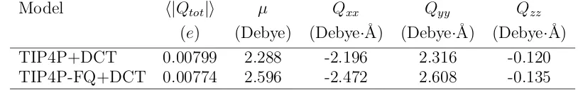
Table 3.3: Average values for the magnitude of the total charge, dipole moment and quadrupole moments of liquid water at a temperature of 298 K and a pressure of 1 atm.

Model h|Qtot|i µ Qxx Qyy Qzz

(e) (Debye) (Debye·˚A) (Debye·˚A) (Debye·˚A)

TIP4P+DCT 0.00799 2.288 -2.196 2.316 -0.120

TIP4P-FQ+DCT 0.00774 2.596 -2.472 2.608 -0.135

The optical dielectric constant, ∞, for the TIP4P+DCT model equals 1 because it

is not a polarizable model. For the TIP4P-FQ+DCT model, ∞ is 1.540±0.002, smaller

than the value for the TIP4P-FQ model (1.592)[7] and the experimental value (1.79).[134]

Two notable differences between the models with and without charge transfer are the heat

capacity, Cp, and the coefficient of thermal expansion, αp. Both properties are smaller for

the charge transfer models than a corresponding model without charge transfer, as seen by

a comparison of the TIP4P+DCT and TIP4P, TIP4P-Ew, and TIP4P/2005 models and of

the TIP4P-FQ+DCT and TIP4P-FQ models. Charge transfer acts to reduce the change

in the energy and density with temperature. The density as a function of temperature

(36)

(37)

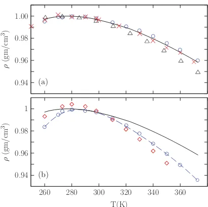
184507-6 A. J. Lee and S. W. Rick J. Chem. Phys.134, 184507 (2011) (a) 0.94 0.96 0.98 1.00 ρ (gm/cm

3) ◦ ◦◦ ◦ ◦ ◦ ◦ ◦ ◦ _◦ ◦ ◦ ◦ × × × × × ×× × × × × _× × (b) 0.94 0.96 0.98 1

260 280 300 320 340 360 T(K)

ρ

(gm/cm

3) ◦ ◦◦ ◦ ◦ ◦ ◦ ◦ ◦

◦ ◦

◦

FIG. 2. Density of (a) TIP4P+DCT (circles), TIP4P/2005 (see Ref.66), and TIP4P-Ew64_{and (b) FQ+DCT (circles and dashed line) and} TIP4P-FQ (see Ref.83) compared to experiment (solid line) (see Ref.78).

TMD values. The TIP4P/2005 and AMOEBA models give a temperature dependence closest to experiment, along with TIP4P+DCT.

The average charge on a molecule,_!_|Qtot|", in the room temperature liquid is about 0.008 e (see TableIV), as given by both charge transfer models, which is less than the mod-els give for the hydrogen bonded dimer (0.020 e). On aver-age there is less overall charge transfer for a water molecule in the bulk liquid than there is for the dimer. Charge trans-fer occurs for the hydrogen bonded dimer because there is asymmetry between the two molecules as one donates and one accepts a hydrogen bond. In the liquid, each molecule is in a more symmetric local environment. If a water molecule has the same number of hydrogen bonds as a donor and as an

TABLE V. Liquid densities at a pressure of 1 atm, compared to experiment (Ref.78).

Density (g/cm3₎

T(K) TIP4P+DCT TIP4P-FQ+DCT Experiment

260 0.9951_±0.0009 0.9823_±0.0024 0.9970 270 0.9989±0.0008 0.9943±0.0014 0.9995 273 0.9988±0.0009 0.9977±0.0014 0.9998 280 0.9996±0.0005 0.9988±0.0013 0.9999 290 0.9989±0.0008 0.9979±0.0013 0.9988 298 0.9977±0.0008 0.9968±0.0006 0.9971 310 0.9942±0.0008 0.9910±0.0007 0.9933 320 0.9906_±0.0008 0.9847_±0.0008 0.9884 330 0.9868±0.0005 0.9772±0.0003 0.9848 340 0.9815_±0.0005 0.9682_±0.0004 0.9795 350 0.9753±0.0005 0.9593±0.0005 0.9737 360 0.9693±0.0005 0.9491±0.0003 0.9673 373 0.9598±0.0005 0.9357±0.0004 0.9584

0 0.1 0.2 0.3 0.4 0.5 0.6 0.7

–3 –2 –1 0 1 2 3

Probabilit

y

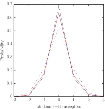
hb donors−hb acceptors

FIG. 3. Probability distribution of the difference in the number of hydrogen bonds a molecule forms as a donor and as an acceptor at three different tem-peratures, 273 K (dashed line), 298 K (solid line), and 373 K (dotted line) from the TIP4P+DCT potential.

acceptor, our model will assign that molecule a zero charge. Fluctuations in the liquid structure give rise to configurations in which a molecule has an unequal number of donor and ac-ceptor hydrogen bonds. The distribution of the difference be-tween the hydrogen bonds, a molecule makes as a donor and as an acceptor is shown in Fig.3for three different tempera-tures using the TIP4P+DCT potential. [Here, we are defining a hydrogen bond as existing if the OH distance between two molecules is less than 2.55 Å, which is half the distance be-tweenr1andr2, see Eq.(1).] Most molecules (about 0.64 or a little less than 2/3 of them at 298 K) form an equal num-ber of donor and acceptor hydrogen bonds. Those molecules would be given a charge of zero by the DCT models. Only a minority of molecules (a little more than a third of them at 298 K) have a charge. As the temperature increases, the hy-drogen bond distribution gets wider, more water molecules have an asymmetric hydrogen bond structure, and!|Qtot|" in-creases. At 273 K,_!_|Qtot|"is 0.0068 e and at 373 K,!|Qtot|" is 0.0103 e. The results are similar for the TIP4P-FQ+DCT model.

IV. CONCLUSIONS

We have presented a new method for treating charge transfer and developed optimal parameters for two different water potentials. The method is general enough that it can be added to a variety of potentials, which we demonstrated by combining it with both a polarizable and a non-polarizable model. The method is simple to implement and, because charge transfer is determined from local geometry only, find-ing the charge of a molecule does not require minimizfind-ing an energy or solving a self-consistent set of equations by iter-ation or other methods. The method can be constructed to give physically reasonable amounts of charge transfer, with-out giving rise to unphysical behavior like transferring charge Figure 3.2: Density of (a) TIP4P+DCT (circles), TIP4P/2005[2](crosses), and

TIP4P-Ew[3](triangles) and (b) TIP4P-FQ+DCT (circles and dashed line) and TIP4P-FQ[4] (dia-monds) compared to Experiment[5](solid line).

Table 3.5: Liquid densities at a pressure of 1 atm, compared to experiment.[5]

T (K) Density (g/cm3₎

TIP4P+DCT TIP4P-FQ+DCT Experiment

260 0.9951_± 0.0009 0.9823_± 0.0024 0.9970

270 0.9989± 0.0008 0.9943± 0.0014 0.9995

273 0.9988_± 0.0009 0.9977_± 0.0014 0.9998

280 0.9996± 0.0005 0.9988± 0.0013 0.9999

290 0.9989_± 0.0008 0.9979_± 0.0013 0.9988

298 0.9977± 0.0008 0.9968± 0.0006 0.9971

310 0.9942_± 0.0008 0.9910_± 0.0007 0.9933

320 0.9906± 0.0008 0.9847± 0.0008 0.9884

330 0.9868_± 0.0005 0.9772_± 0.0003 0.9848

340 0.9815_± 0.0005 0.9682_± 0.0004 0.9795

350 0.9753_± 0.0005 0.9593_± 0.0005 0.9737

360 0.9693_± 0.0005 0.9491_± 0.0003 0.9673

373 0.9598± 0.0005 0.9357± 0.0004 0.9584

(38)

maximum near the experimental value of 281 K.[5] The TIP4P+DCT model is very accurate

over the whole range of temperatures for which the liquid is stable. Also shown in Figure

3.2(a) are the results for the TIP4P-Ew and TIP4P/2005 models – two of the models which

best reproduce the liquid density over this temperature range and give a value of αp closest

to experiment. The TIP4P-FQ+DCT model gives an improvement over the TIP4P-FQ

model for the density at higher temperatures and near the density maximum. In addition

to the TIP4P-Ew, TIP4P/2005, and TIP4P-FQ models, a number of water models give a

temperature of maximum density (TMD) near 281 K, including TIP5P[129], TIP5P-E[121],

AMOEBA[130], the 6-site Nada and van der Eerden model[135], PPC[108], BSV[136], and

TIP4P-Pol2.[111] Many of these models, like TIP4P+DCT, were optimized to reproduce this

property.[2, 3, 121, 129, 135] Many commonly-used models do not have a TMD above 250K

or a TMD not close to 277 K including TIP4P, TIP3P, SPC,[137] and SPC/E.[138, 139]

Interestingly, all these models tend to overestimate αp, giving a density that changes too

much with temperature, even those with fairly accurate TMD values. The TIP4P/2005

and AMOEBA models give a temperature dependence closest to experiment, along with

TIP4P+DCT.

The average charge on a molecule, _h|Qtot|i, in the room temperature liquid is about

0.008 e (see Table 3.3), as given by both charge transfer models, which is less than the

models give for the hydrogen bonded dimer (0.020 e). On average, there is less overall

charge transfer for a water molecule in the bulk liquid than there is for the dimer. Charge

transfer occurs for the hydrogen-bonded dimer because there is asymmetry between the two

molecules as one donates and one accepts a hydrogen bond. In the liquid, each molecule

is in a more symmetric local environment. Fluctuations in the liquid structure give rise to

configurations in which a molecule has an unequal number of donor and acceptor hydrogen

bonds. The distribution of the difference between the hydrogen bonds a molecule makes as

a donor and as an acceptor is shown in Figure 3.3 for three different temperatures using

Theoretical Approaches to the Characterization of Water, Aqueous Interfaces, and Improved Sampling of Protein Conformational Changes

ScholarWorks@UNO

ScholarWorks@UNO

Theoretical Approaches to the Characterization of Water,

Theoretical Approaches to the Characterization of Water,

Aqueous Interfaces, and Improved Sampling of Protein

Aqueous Interfaces, and Improved Sampling of Protein

Conformational Changes

Conformational Changes

Acknowledgments

Table of Contents

List of Figures

List of Tables

Abstract

Chapter 1

Introduction

Chapter 2

Background and Theory

2.1

Potential Energy Models and Force Fields

2.2

Obtaining Molecular Data

2.3

Molecular Dynamics Simulations

2.4

Water Potentials

Chapter 3

The Effects of Charge Transfer on the Properties of Liquid

Water

3.1

Introduction

3.2

Methods

3.3

Results and Discussion