in the population sciences published by the Max Planck Institute for Demographic Research
Doberaner Strasse 114 · D-18057 Rostock · GERMANY www.demographic-research.org
DEMOGRAPHIC RESEARCH
VOLUME 3, ARTICLE 3
PUBLISHED 4 AUGUST 2000
www.demographic-research.org/Volumes/Vol3/3/
DOI: 10.4054/DemRes.2000.3.3
A Search for Aggregate-Level Effects of
Education on Fertility,
Using Data from Zimbabwe
Øystein Kravdal
A Search for Aggregate-Level Effects of Education on Fertility,
Using Data from Zimbabwe
Øystein Kravdal 1
Abstract
The analysis was based on the 1994 ZDHS combined with aggregate data from the 1992 census. Discrete-time hazard models for first and higher-order births were estimated for 1990-94. The average length of education in the district and the proportion who are literate were found to have no impact on a woman’s birth rate above and beyond that of her own education, when it was controlled for urbanization. This was the case for women who themselves had little or no education as well as for the better-educated. So far, no significant influence of aggregate education on fertility has been well documented in the literature either. However, in this study, aggregate-level effects appeared in models for fertility desires and contraceptive use among married women with at least one child.
1 Department of Economics, University of Oslo, P.O. Box 1095 Blindern, N-0317 Oslo, Norway
1. Introduction
Although women’s education has been one of the most thoroughly studied determinants of fertility, with the perspective now often extended to include the closely related ‘women’s position’, the research area is still far from being exhausted. For example, several causal links seem plausible in light of existing empirical evidence, but we have a meagre knowledge about their relative importance. The differences in education effects across settings also deserve further exploration. Another, and not so widely recognized challenge, is to find out whether education at the aggregate level has any effect on a woman’s fertility above and beyond that of her own education. The possible importance of ‘mass education’ was discussed by Caldwell [Caldwell 1980] many years ago, and has occasionally been touched in more recent reviews (see e. g. [Cleland and Jejeebhoy 1996]), but little empirical evidence has so far been accumulated.
When the intention is to assess how expansion of education, which of course is a goal itself, influences fertility, one obviously needs to estimate effects of a woman’s own education. In addition, there may be a ‘spill-over’ from other people’s education through, for example, social learning. Uneducated women who live in societies where a large proportion are literate, or where the average educational level is high, may have a fertility different from that of uneducated women elsewhere. Also the better-educated may be influenced by the educational distribution in the community. If aggregate education has, on the whole, a substantial depressing effect, fertility will decline more sharply in response to an increase in women’s education than suggested by the estimates of individual-level effects.
It would clearly be important to try to quantify this aggregate-level contribution. This calls for the inclusion of both individual and aggregate measures of education in multilevel models (along with some control variables that are determinants of education, of course). As illustrated below, the individual-level models usually estimated will capture part of the aggregate-level effect, in addition to the purely individual one, but not the full effect.
Many researchers have included individual and structural characteristics simultaneously in regression models for reproductive behaviour, with or without the use of statistical tools specially developed for multilevel analysis. Not least the impact of family planning facilities in the community has attracted interest (see e.g. [Entwisle et al 1997]). However, very few have provided statistically well-founded assessments of how aggregate education influences fertility.
Lesthaeghe et al. [Lesthaeghe et al 1985] searched for effects of aggregate education, using both a measure of cumulated fertility and some proximate determinants as dependent variables. Some main or interaction effects showed up, but the close link between education and urbanization was not taken into account in this study either. Similarly, Hirschman and Guest [Hirschman and Guest 1990] estimated a significant fertility-inhibiting effect of the proportion of women with post-primary education in four Southeast Asian countries, but without an urban/rural control variable.
In a more recent study, Thomas [Thomas 1999] reported that mean educational level in the community had a significant depressing effect on the number of children ever born in South Africa. Unfortunately, he did not show the size of this effect. Moreover, a Tanzanian study by Kravdal [Kravdal 2000] provided indications that higher-order birth rates were relatively low in regions where many women were literate, whereas sharper such effects appeared in a model for contraceptive use. A similar result for contraceptive use was reported by Amin et al. [Amin, Diamond and Steel 1996], who estimated the influence of the proportion literate women in various districts of Bangladesh.
It is not unlikely that such aggregate effects are different for educated and uneducated women, one way or the other. This is, of course, equivalent to saying that the individual effect of education may depend on the general educational level. Very little is known about such context-dependence. Jejeebhoy [Jejeebhoy 1995] reviewed several studies of mixed character and quality from countries with different overall educational level, without arriving at a very clear conclusion, and only some of the original multilevel studies referred above included tests of cross-level education interactions. The main objective of this analysis was to find out whether various measures of aggregate education have had an effect on fertility, net of the individual education, and with control for urbanization. As part of this, the differential impact across women’s own education was also addressed. Contrary to some of the above-mentioned studies, where cumulated fertility was the dependent variable, the focus here has been on recent births in a hazard model approach. This means that the available cross-sectional data on aggregate education were more relevant in terms of place and time. Moreover, models were estimated for fertility desires, contraceptive use and post-partum insusceptibility due to lactational amenorrhoea or sexual abstinence in order to build up a more complete picture. These important determinants of fertility may respond differently (also) to aggregate education. As very common in studies of education and fertility, only women’s education was included in the models. In a final section, however, the importance of husbands’ and men’s education will be briefly dealt with.
2. Theoretical considerations
2.1 A Brief Review of Suggested Individual-Level Effects of Education
There are several plausible reasons why women with, for example, some secondary education usually display a lower fertility than the uneducated. To summarize very briefly, and without pretending to produce a complete list of mechanisms, fertility desires have been thought to be influenced by the individual woman’s education because of: i) the high opportunity costs of childbearing involved in some types of work that may be offered to the better-educated women, ii) the cash expenses and children’s reduced contribution to domestic and agricultural work as a result of children’s schooling, which tends to be encouraged by educated mothers, iii) the reduced need for children as old age security, or to support the woman even as a relatively young widow, when the family’s wealth allows other kinds of savings, or when the woman is able to earn a living on her own and even set something of that aside for the future, iv) the higher prevalence of nucleated families, which may reduce fertility partly because childbearing costs to a larger extent must be covered by parents, v) a stronger desire to spend more time caring for a child and to invest more in each child, not only in terms of education, vi) stronger preferences for consumer goods or other sources of satisfaction, and vii) a lower infant and child mortality, influencing desires through replacement and insurance effects. These fertility-inhibiting effects may be set off against viii) a possibly stimulating impact of a higher purchasing power resulting from educated women’s own work or their marriage into a relatively rich family [Note 1].
Mortality has a bearing also on the supply side. Besides supply and regulation are likely to be influenced by education, one way or the other, because of ix) the higher age at marriage among the better educated, x) their knowledge about and accept for modern contraception, and their ability to use it efficiently, as well as their more efficient use of traditional methods because of better knowledge about their own body, xi) the erosion of traditional norms about post-partum sexual abstinence and breastfeeding that is supposed to go hand in hand with education, and xii) their higher fecundity because of better health or treatment for sexually transmitted diseases. As widely known, the fertility-stimulating effects have actually been dominant at a moderate educational level in many countries, and in particular in Africa during the 1970s and early 1980s.
cultural proscriptions (see e.g. [Niraula and Morgan 1996]). In other words, her own current position compared to men, and that she expects for the future and for her daughters, are probably determined both by gender attitudes and structures in society and such individual characteristics as her own education. If she has an education, she may, for example, be allowed by the family to work outside the house and more often be heard in discussions with husband or in-laws [Note 3]. This will add to the effect of her literacy and skills and possibly reduce fertility desires through such factors as opportunity costs, old age security concerns and child mortality.
Women’s status may also operate through channels other than those listed above. For example, in situations where the husband wants more children than the wife, a strengthening of women’s decision-making autonomy will reduce fertility [Note 4]. Besides, when a wife is considered more of an equal than a subordinate, the couple may communicate better about contraception, and the husband may see more clearly how childbearing burdens the wife. On the other hand, such a relationship may stimulate sexual activity. As a third example, women who themselves have a relatively inferior position relative to men may not only consider the childbearing costs generally low and the rewards high, but expect boys to be even more useful than girls [Note 5]. This will enhance fertility desires in settings where fertility is not extremely high.
While such status effects seem theoretically plausible, however, the quantitative empirical evidence is still quite weak.
2.2 The Possible Importance of Others’ Education
Several of the causally intermediate factors mentioned above may depend not only on the woman’s own education, but also on that of other women. As pointed out by, for example, Montgomery and Casterline [Montgomery and Casterline 1996], other women may exert an effect because of social learning, social influence and more indirect mechanisms. The individual woman may learn directly from others by communication and observation. It is not only factual knowledge that is likely to be transmitted, but also attitudes as well as understanding of possible consequences of different actions. Bongaarts and Watkins [Bongaarts and Watkins 1996] have stressed that this learning may include interpretation in light of current local conditions and the individual situation. There may also be a more passive imitation of behaviour (‘social influence’) without any (active digestion of) new knowledge, driven by a desire to attract other people’s approval. A more indirect mechanism is that others’ ideas, resources or behaviour can influence society and social institutions and thereby also behaviour more generally.
negative, and may differ between women who themselves have little education and those who are better-educated.
To be more specific, one possibility is that uneducated women may have more knowledge of contraception and more modern views about its acceptability if they live in a society where many women have attended school for some years than if they live elsewhere. They may also simply tend to imitate the more widespread use of contraception among the better-educated. Moreover, their preference structure and their practice of breastfeeding and post-partum abstinence may be influenced by aggregate education.
Other people’s education may be of importance also to those who themselves have more education, although for slightly different reasons. A diffusion of factual knowledge of contraception is, for example, less relevant, but there may be a more efficient interpretation of the ideas and attitudes the better-educated have been exposed to at school, through reading or because of interaction with people elsewhere if there are more women to share these experiences with.
An argument along similar lines has been advanced by Caldwell [Caldwell 1980], who suggested that ‘mass education’ will make everyone more conscious about the need to educate their children, and that it will strengthen Western middle class values, with more emphasis on individual rights than on the duty to a larger family network. His hypothesis is that an increase in the proportion who are literate, from a very low level, is the most crucial change, whereas the average length of education among the literate is of less importance. Apparently, he did not consider the differentials in such macro effects, but it seems most plausible that the (large majority of) uneducated would be most influenced.
Moreover, opportunity costs of childbearing may depend on other people’s education. Generally, having a high education will increase a woman’s chance of finding a relatively well-paid job (where she cannot bring her children with her). However, under the assumption of a fixed supply of such jobs, a high proportion of well-educated women in the community will decrease her chance. To elaborate on this, even women with a quite short education may be able to get into this niche in the labour market when few have an education, whereas their situation would be little different from that of the uneducated when the average education is higher.
In other words, if the temporal dimension is disregarded for simplicity, it can be concluded that a high average education may reduce the opportunity costs because of a competition effect and add to them because of increased supply and acceptance of well-paid jobs. To complicate this further, opportunity costs may be substituted by direct costs by purchasing child care, which is likely to be particularly cheap when only a few women work away from home.
Of course, if a general rise in women’s education (with or without an accompanying rise for men, which is addressed below) contributes to undermine old ideas about women’s rights and obligations compared to men, it is not only the opportunity costs of childbearing that will be enhanced. An improvement of women’s status as a contextual phenomenon, and the changes in women’s individual position that follow in the wake of this, may influence fertility for many other reasons, a few of which were reviewed above. This may influence also the fertility of women who themselves have little education.
Besides, broader economic transformations are likely to take place as a result of a better-educated work force, in the long run. In addition to the increase in the number of well-paid jobs in the modern sector, as referred to above, it is, for example, plausible that the agriculture will be generally modernized, including that among uneducated farmers. This will undermine children’s relative importance in the fields, and thus the incentive for childbearing. Moreover, higher productivity in agriculture, combined with a general knowledge level that may facilitate the establishing of manufacturing industries that benefit particularly strongly from economies of scale, may lead to an increased concentration of people in urban areas. In other words, it can be argued that investments in education in a district may contribute to stimulate the urbanization of that district, although very slowly. Also the generally higher wealth that is likely to be a part of these transformations may have an effect on fertility, although not necessarily a positive one.
As yet, there is no clear empirical evidence about interactions between individual and aggregate education. Jejeebhoy [Jejeebhoy 1995] concluded that, in countries where women’s literacy is high, primary education is more likely to push fertility down, and the negative effect of secondary education is particularly sharp. This is, of course, the same as claiming that the literacy rate has the clearest negative effect among the better-educated women. Her conclusion was based on a review of a number of studies with different, and more or less relevant, control variables included, and its conclusion did not have a very solid basis. She found, for example, that fertility
desires responded most sharply to secondary education in the countries with a generally low
2.3 Determinants of Education
In order to find out how investments in a woman’s education will influence her fertility, one must, of course, estimate models that include various individual and structural factors that both are determinants of education and, for other reasons, influence fertility. For example, the individual woman’s education is likely to be determined by resources and attitudes in her family of origin as well as society’s needs for and ability to finance education and the general attitudes towards women’s schooling. These aggregate factors, which may well differ across the country, are of course also determinants of men’s and other women’s education.
More specifically, people’s educational level probably depends strongly on whether they live in urban or rural areas. The more advanced economy in cities both requires and allows investments in education, and returns to investments may be high because of the higher population density. This calls for the inclusion of an urban/rural variable in the models, which the Zimbabwean data allowed. (According to the 1994 ZDHS, 29 per cent lived in urban areas). The fact that there may also be a reverse relationship of presumably less importance, with aggregate education fuelling urbanization in the long run, is returned to below.
The data include no relevant information about the family of origin, but the woman’s own religion can be supposed to be a stable, often socially inherited, characteristic that has a bearing on decisions related to her education (although the opposite causality cannot be completely excluded). (55 per cent of the Zimbabwean population are Christian, according to the 1994 ZDHS).
Unfortunately, it was not possible to control for the general attitude towards women or the economic wealth in the districts. The implications of this are also discussed below.
3. Data and methods
3.1 Data
The 1994 ZDHS, which is the main data source for this study, has a sample of 6128 women living in 230 census enumeration areas (‘clusters ’), who were interviewed between July and December 1994 [Central Statistical Office 1995]. The survey also includes a ‘service availability’ module on family planning facilities in or in the vicinity of each enumeration area. The latter data were not used in this analysis because of a presumably spurious relationship with education. (Another problem is that initiatives to improve access to contraception in some areas by setting up clinics or outlets or organizing community-based distribution to some extent may be a response to fertility or assumed fertility desires, see e.g. [Angeles, Guilkey and Mroz 1998]).
In the ZDHS survey, the 10 provinces of Zimbabwe were divided into urban and rural areas (except Bulawayo and Harare, which are almost completely urban) to form 18 strata. A set of 2-30 enumeration areas were supposed to be representative of these strata, but stratum-specific weights had to be used to obtain representativity at the national level.
The 10 provinces consist of a total of 70 districts. Aggregate data for each of these districts were taken from the 1992 Population Census publications [Central Statistical Office 1993] and linked to the survey file by means of a list of district identifiers for each enumeration area (provided by the Central Statistical Office on request). (Macro data at the enumeration-area level could only have been established by aggregating from the ZDHS, which did not seem to be worthwhile, because there were less than 30 respondents in each area on average).
3.2 Definition of Education
In this study, five categories were defined for women’s educational level: i) no education or incomplete primary education lasting less than 3 full years, ii) incomplete primary education of longer length (3-6 years), iii) complete primary education or incomplete secondary education of less than 2 full years (excluding the 7 required for primary education), iv) secondary education of 2-3 years, and v) secondary education of 4 or more years. These categories for duration of schooling were chosen to fit with the published aggregate data from the 1992 census.
districts) in order to get a national average proportion equal to that reported for 15-50 year old women in the ZDHS survey. The proportions in the other educational categories were scaled up or down similarly (using other constants, in order to fit with national ZDHS averages). After this procedure, the sum of proportions over the 5 educational categories in the different districts deviated only slightly from 1 (while it, of course, was exactly 1 at the national level). This was corrected by multiplying all proportions with the same district-specific constant. The result of this approach is that cross-district differences in educational distributions across districts are determined by the census data, while the overall level is determined by the survey data. (The reason why the survey data were not used as the only data source was, of course, the relatively small number of observations even within a district). Such an adjustment will have some influence on the point estimates of aggregate education effects, but leave little imprint on significance levels.
The main representation of aggregate educational level in this study was the average years of schooling. In addition, measures of breadth and depth of education, defined as proportion literate and average years of schooling among the literate, were used. Unfortunately, the very strong correlation between the latter two variables did not allow estimation of separate effects. They were instead considered as two alternative specifications. When these averages were calculated, the years of schooling in the five different categories defined above were set to 1, 4.5, 7.5, 9.5 and 12.
3.3 Discrete-Time Birth Rate Models
Discrete-time hazard regression models for the period January 1990 - June 1994 were estimated from the birth histories in ZDHS. Each person contributed a series of 3-month observation intervals. Tests showed this to be a sufficiently short interval. First and higher-order birth rates were modelled separately, in recognition of the widely different individual decisions and social processes involved in entry into parenthood and subsequent parity transitions. In first-birth models, follow-up started at age 14, unless this age was reached before 1990. After first birth, multi-episode models for the transition into a higher parity level were estimated, with observation intervals running from the time of first birth, or from 1990, if the first birth was before that.
and for certain educational levels. For example, the estimated effects of a short secondary education will be biased only for early teenage years, when attending the first part of secondary school is still an option. Primary education takes place too early to be influenced by childbearing, and higher-order birth models are not hampered by such problems, because, at this stage, few women would take further education anyway. It was experimented with models where both enrollment and educational level (lagged one year) were included, on the basis of an assumption that school attendance is continuous from age 6.This gave very similar results.
3.4 Migration as a Complicating Factor
In birth rate models for 1990-94, it would be most relevant to include the educational distribution in the district in which the women lived during that period or before (because their surroundings at an earlier age may have had a lasting influence on, for example, their attitudes). Fortunately, the data available in this study came close to allowing this. They provided information about the educational distribution of the district in which the women lived at interview in 1994, and where the large majority must have lived also the previous five years. As explained above, the educational data were for a combination of 1992 (measurement of district variation) and 1994 (measurement of overall level).
3.5 Models for Fertility Desires, Post-Partum Susceptibility and Contraceptive Use
Special interest is, of course, attached to the birth rates, but the data also allow a check of how important determinants, such as fertility desires, post-partum susceptibility and contraceptive use, are influenced by aggregate education.
Logistic models for the probability of wanting another child within two years, for the probability of being susceptible, and for the probability of using modern contraception were estimated for women who were married (including those who reported less formal unions) at interview, and who were non-pregnant and had at least one child at that time. A considerable proportion of these women, including those in monogamous unions, reported that their husband lived elsewhere, but they were not considered a separate group in the analysis.
Susceptibility was defined as having had intercourse during the last month before interview and not being amenorrhoeic [Note 7]. The susceptibility models were further restricted to mothers of children younger than 2 years.
Two types of contraceptive-use models were estimated. One of the models was restricted to women who had been sexually active during the last month, who were neither infecund nor amenorrhoeic at interview, and who reported that they did not want another child within the next two years (although also those who want a child so soon may use contraception, in order to avoid an immediate pregnancy). In the other model, there were no such conditions. Many studies, including that by Amin et al. [Amin, Diamond and Steel 1996], have been based on such a model exclusively, which means that one cannot know whether low contraceptive use is due to little need for contraception or a poor ability to satisfy a substantial need.
3.6 Multilevel Models
4. Main Effects of Aggregate Education on Birth Rates
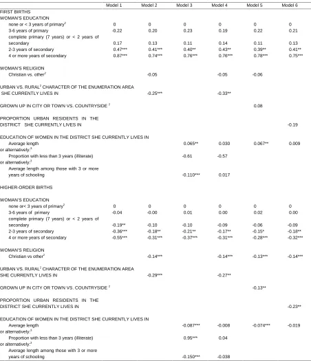
According to models where only age, parity and duration since previous birth were included along with individual education, a complete primary education does not reduce first-birth rates significantly at the 0.05 level. However, the effect on higher-order birth rates was found to be significant. The point estimates (log odds) were -0.17 and -0.19, respectively (Model 1, Table 1). This is for the period 1990-1994 and is quite consistent with the difference of 0.5 in TFR between uneducated women and those with a primary education that is shown in univariate tabulations (covering the last few years before the survey) from the 1994 ZDHS [Central Statistical Office 1995] [Note 9].
The effects of secondary education were significant for both first- and higher-order birth rates. If short and long secondary education were combined, the point estimates were about 0.70 and -0.45, respectively (not shown). This accords reasonably well with the TFR difference of 1.9 between uneducated women and those with at least some secondary education that was reported from the 1994 ZDHS.
(Table 1 about here)
When average length of education was included, the effects of individual educational level were reduced (Model 3). The effects of aggregate education were significant in these simple models. In order to get an impression of the relative importance of aggregate and individual effects, the consequences of changing the educational distribution for women aged 15-50 were predicted. Such distributions are shown in Table 2 for some groups of districts. For example, it is easy to calculate that, if the educational distribution is changed from that in the bottom-10 districts to that in the top-10 districts, the individual contributions will be -0.32 for first births and -0.14 for higher-order births [Note 10], whereas the aggregate contribution associated with this increase of about 2.5 years in average education will be -0.16 and -0.21, respectively. It should also be noted that the sums of individual and aggregate contributions are markedly higher than the corresponding predictions of -0.35 and -0.22 based on models with only individual education included. In other words, when it is taken into account that educated women tend to live in areas with many other educated women, the effect of individual education is reduced, but this is more than compensated for by the aggregate effect. This is the same as saying that, when only individual education is included in the model, part of the aggregate effect is also captured, but not the entire [Note 11].
It should also be noted from Model 3 that first-birth rates were more clearly influenced by the depth of education than its breadth (the latter effect was almost significant at the 0.10 level). For higher-order births, however, both effects were significant.
The estimates presented above grossly overstate the causal impact on fertility of individual investments in education. When it was taken into account that educated women tend to have a Christian background, and that their education, as well as that of other women in the district, must be determined partly by the urban/rural character of the enumeration area they currently live in, effects of education were markedly reduced. Individual effects were left almost unchanged for first births and slightly reduced for higher-order births, whereas aggregate effects no longer were significant (Model 4). Also the point estimates of the latter were very small. An increase of, say, 2.5 years in average education would increase first-birth rates by 0.08 and decrease higher-order birth rates by 0.02, which is completely negligible compared to individual effects. In fact, aggregate education might just as well have been left out of the models. When only urban/rural and religion were included, and not aggregate education, one was left with the same impression of effects of investments in education (Model 2). (As further illustration of the importance of these control variables, the impact of the above-mentioned change in the educational distribution would be about 1/3 weaker according to Model 4 than according to the simpler Model 1, which corresponds to univariate TFR tabulations).
Moreover, experiments with various specifications clearly showed that the results depend markedly on the kind of urban/rural variable that is used. Because a woman’s individual education may have been determined more by the place of residence where she grew up than by the place where she currently lives, it would seem quite reasonable to include the urban/rural nature of the former. However, adding this variable to the simplest model had much less impact on individual education effects (not shown) than adding an urban/rural variable referring to the current place of residence. Moreover, aggregate effects remained almost unchanged (Model 5), because this urban/rural variable is less closely linked with the aggregate education of the district in which she currently lives.
The aggregate education is a district-level variable. Living in an urban enumeration area does not necessarily mean that the district is generally very urbanized. For that reason, one might alternatively have preferred to include the proportion urban residents in the district. This would have reduced aggregate effects of education very markedly (Model 6), although not quite as much as the inclusion of an urban/rural variable referring to the enumeration area (Model 4).
As yet another alternative, the character of the current place of residence was grouped into more categories by considering the rural enumeration areas’ distance to cities. This gave only slightly smaller effects of education than in Model 4 (not shown).
Some models were therefore estimated separately for rural areas. No significant effects of aggregate education appeared in these models either, except that depth of education was almost significant at the 0.10 level for higher-order births (not shown).
To summarize, the results provide very little support for the idea that there may be an extra stimulus to fertility decline through effects of aggregate education (i.e. at a given individual educational level). The lack of access to control variables should not weaken this conclusion much. If the general educational level is strongly determined by structural factors that have a clear stimulating effect on fertility, its true effect, net of urbanization, would be negative, but this is not very plausible. Such background factors are more likely to have a fertility-inhibiting effect, if any. A negative effect of aggregate education only seems reasonable to the extent that investments in education in a region contribute to stimulate the urbanization of that region, which must be a very slow process.
The latter comment may need an elaboration: It was explained above that the urban/rural character of the community is likely to be a determinant of aggregate education. This means that the estimated effect of aggregate education, when both variables are included, can be interpreted as the total effect of that variable (assuming also that none of the other regressors are causally intermediate). If it had been more appropriate to consider urbanization a consequence of education, the interpretation would have been different. In that case, the aggregate education effect estimate would reflect the direct effect of that variable, while there would also be an indirect one operating through urbanization. The size of the latter would be determined by the effect of aggregate education on urbanization (not estimated) and the effect of urbanization on fertility. The sum of these contributions, i.e. the total effect, could, of course, more easily have been estimated by leaving the urban/rural variable out. This reverse causality may hold some truth, without being very dominant. It is certainly possible that investments in education may stimulate urbanization, although it is not a result that is likely to be seen very soon after the school system is expanded. In other words, the total effect of aggregate education may, in the long run, be slightly more negative than suggested by the aggregate education effect estimate from a model where both variables are included.
5. Macro-Micro Interactions in Birth Rate Models
The fact that there are no main effects of aggregate education does not exclude the possibility of interaction effects, because the effect of a high average educational level might, in principle, be significantly positive for a woman with low education and significantly negative for one with high education, or vice versa. However, more flexible model specifications revealed no such pattern.
The simplest check was to include an interaction term between average length of education (or its deviation from the sample mean of about 7 years, in order to obtain individual effect estimates closer to those shown in Table 1) and length of individual education (transformed into a 0-1 scale to facilitate interpretation). This is a linear interaction, in the sense that each additional year of individual education increases or decreases the impact of aggregate education equally much. According to the point estimates, the impact of an extra year of average education on first-birth rates changes gradually from 0.11 at the lowest individual level to -0.01 (=0.11-0.12) at the highest level, but neither the main effect nor the interaction effect was significant (Model 1, Table 3). The estimates for higher-order births suggested an opposite pattern, but were also very far from attaining significance.
(Table 3 about here)
Some other specifications were also tried. First, aggregate effects were allowed to differ freely across three broad categories of individual education, rather than assuming a linear interaction. No significant effects appeared, and there was no U-shaped pattern indicating that the linear specification was highly inappropriate (Model 2).
Second, the proportion illiterate was included instead of the average education as a main effect and in interaction with individual education. As an alternative, average education among those with more than 3 years of schooling was included. No aggregate main or interaction effects were significant with these specifications (Model 3 and Model 4). Nor did the effects attain significance when the linearity assumption was removed, as in Model 2 (not shown).
Finally, it was checked whether women at low, medium or high education were influenced by the proportion at a higher (if relevant) or lower (if relevant) level. No significant effects were found in these models either (not shown).
Also interactions between urban/rural and individual education were included in these models, but without influencing the cross-level education interactions markedly. In fact, interaction effects were insignificant even when main effects of urban/rural and religion were left out.
6. Other Effects of Aggregate Education
When a model for fertility desires was estimated, with the same control variables as in the birth rate models, a significant negative effect of average length of education appeared (Table 4) [Note 12]. Also breadth and depth of education were found to weaken fertility desires.
(Table 4 about here)
Post-partum susceptibility was found to be independent of aggregate education. The point estimate suggested that women in districts with many illiterate tend to breastfeed longer or more intensely or to resume sexual activity later than women at the same educational level in other districts. This accords with the commonly found impact of individual education (which does not appear clearly in these data), but the effect was far from significant.
When the probability of using modern contraception was estimated for women who did not want another child within the next two years, and who were sexually active, not amenorrhoeic and not infecund, the effect of average education did not reach significant, while that of average education among the literate was significant at the 0.01 level. In accordance with the results for fertility desires, an unconditional model for contraceptive use gave more clearly significant effects of aggregate education. Both models for contraceptive use suggested sharper effects of depth of education than breadth.
Apparently, the bias introduced by considering individuals within a district or enumeration area as independent is minor (and certainly compared with other problems that hamper this and other similar analyses). An ordinary single-level logistic model for fertility desires gave a point estimate of -0.26 for the effect of average education (Table 4), with a standard error of 0.070 (not shown). This result was replicated in a two-level MLwiN model (based on the 1. order MQL algorithm) by using a constant variable as a level-two identifier and constraining the variance at this fictitious level to be 0. When enumeration area or district were instead defined as level two, the variance of the aggregate-education effect estimate only increased to 0.084-0.087 (both according to the 1. order MQL and the 2. order PQL algorithm; not shown). Several similar attempts were made to estimated MLwiN models for contraceptive use, but convergence to plausible estimates was never achieved. The interactions between average and individual length of education were not significant in these demand, supply and regulation models. However, the estimates suggested that the impact of aggregate education on fertility desires is strongest among women who themselves have little education.
child soon. Besides, the interaction between average and individual education was significantly positive (at the 0.05 level) in models for unconditional contraceptive use.
7. The Importance of Husbands’ and Men’s Education
The estimated difference in fertility between women with low and women with high education partly reflects that the former (if married) tend to have a husband with low education and the latter a husband with higher education. Husband’s education may have an independent effect on fertility, stemming from two inseparable components: Given a woman’s education, a higher education for the husband means that the educational gap between the spouses is wider. Besides, husband’s education may have an impact more in its own right. Anyway, the impact of an expansion of women’s education from that in the bottom-10 districts to that in the top-10 districts that was calculated above will only be a good prediction of fertility changes if men’s educational level rises correspondingly (i. e. so that the distribution of men’s education, given that of the woman, is kept constant). In the very hypothetical situation where only women’s educational level is enhanced, women will not on average get better-educated men, but (disregarding the possibility that the marriage intensity generally falls) the degree of homogami will change. For example, women with low education will found it more difficult to get a better-educated husband.
In order to establish a good platform for predicting fertility responses to educational expansion, one should estimate independent effects of men’s and women’s education (at the individual level, as well as the aggregate, as explained below). Lack of couple data is a major obstacle to this. DHS surveys and similar sources typically include information about the husband of currently married women, but not about the education of the husband at previous points of time.
In this study, an impression of the importance of controlling for husband’s education is provided by simply restricting the higher-order birth model to a sample of women who were married at interview. It is assumed that they have had the same husband throughout the five-year period of analysis. Women in this sample may well be selected for high fertility, for example because divorce may be partly a result of low fertility, but the effects of education are not necessarily severely biased. That depends on whether the link between education and fertility depends markedly on (changes in) marital status.
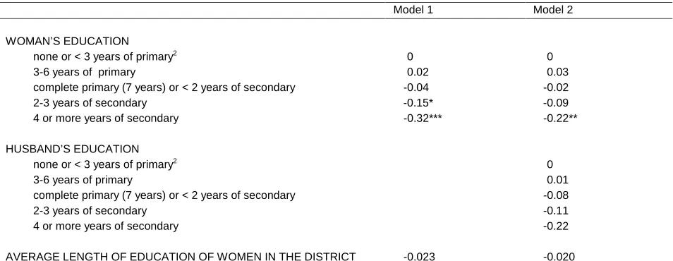
Fortunately, when the sample was restricted in this manner, effects of women’s individual and aggregate education were about the same as found for the larger sample (compare Model 1, Table 5 with Model 4, Table 1). A control for husband’s education turned out to be quite important. When that variable was included in the model, the effect of women’s individual education was substantially attenuated (Model 2, Table 5).
(Table 5 about here)
Similarly, the estimates of aggregate education effects reported in Table 1 capture a combined impact of men’s and women’s educational distribution, which in turn can be interpreted both as ‘absolute’ effects and gap effects, as commented above for the individual level. In Zimbabwean districts where women’s education is low, also that of men is low, although not quite as low. In districts where women’s education is relatively high, men’s education is even higher (but with a somewhat smaller gap between the sexes than in the other districts). The aggregate effect of expanding women’s education exclusively will be even less negative than suggested by the estimates in Table 1, unless men’s education at the aggregate level actually stimulates fertility or is without importance.
The impact of women’s and men’s educational distribution partly operates through husband’s education as an individual-level effect. Given a woman’s education, her chance of marrying a man with a high education will probably increase if many men have high education and decrease if many other women have a high education. According to the model estimated with the Zimbabwean data, the already small aggregate effect of women’s education (which also incorporates an effect of men’s education) is slightly reduced when an individual variable for husband’s education is included.
8. Summary and Conclusion
The fact that a woman’s education influences her fertility, and usually negatively, is firmly established, although we still know little about the exact size of the effect in different settings. An additional fertility-depressing effect of the general educational level in the community, net of its aggregate determinants, is certainly not intuitively implausible either. However, such a spill-over effect from educational investments has yet to be well demonstrated empirically.
In this study, a significant negative effect of aggregate education was found for contraceptive use, just as reported by Amin et al. [Amin, Diamond and Steel 1996] in a study from Bangladesh. This reflects in particular the weaker fertility desires among women in districts with many literate women and a high average education, than among women at the same educational level in other districts. Only a negligible counteracting effect was estimated for post-partum susceptibility.
Nevertheless, actual birth rates the five years before interview were found to be unaffected by other persons’ education (with the same control variables included in the models). Significant negative effects appeared only in birth rate models where the urban/rural character of the current place of residence was not included. (With the model specifications chosen in this study, it was easy to get an impression of the relative importance of aggregate education, and it was indeed large according to these simplest birth rate models.) This illustrates the weakness of some previous studies, where negative effects of aggregate education were found, but without controls for urban/rural differences. In fact, the present study has also demonstrated that the choice of urban/rural control variable can be quite critical.
The educational distribution is, of course, closely linked with a wide range of structural factors other than urbanization. When the intention is to assess the total effect of educational expansion, one should include in the models measurements of those of these structural factors that are determinants rather than consequences of education. However, the direction of causality is inherently blurred. Had it, for example, been possible to control for women’s general position compared to men, which may well differ across the country, the effect of aggregate education on fertility desires might have been attenuated (or become completely negligible, implying that, in districts with more egalitarian ideas about gender roles, people would have wanted few children regardless of education). On the other hand, the educational distribution is likely to feed back on women’s position, in the long run, so the total impact might be more clearly negative than suggested by estimates from models with such a variable included.
individual educational level) only seems reasonable to the extent that investments in education in a region contribute to stimulate the urbanization of that region, which must be a very slow process. The fact that a significantly negative aggregate effect failed to show up in these Zimbabwean fertility models does not mean that such an effect is generally non-existent. One cannot, of course, reject that possibility that richer regional data for Zimbabwe might have revealed effects. It is also possible that stronger effects would have been found in countries with much lower literacy rates. According to Caldwell, it is the impact of introducing compulsory education in a society where almost everyone is illiterate that is most pronounced. However, most countries are far beyond this level now, so a similar analysis of such a change would be difficult to make. Besides, this study has cast some doubt on the idea that breadth of education is more important than depth.
No significant interaction effects between individual and aggregate education appeared in the Zimbabwean data. The point estimates did not even display a systematic pattern, but weakly suggested that the negative effect of aggregate education that was found for fertility desires may be confined to women at a low educational level. Changing the perspective slightly, this lack of a clear interaction pattern for birth rates implies, of course, that individual effects of education are independent of the aggregate level. This is a noteworthy conclusion in light of the currently strong scholarly interest in context dependence.
9. Acknowledgements
Notes
1. Theoretically, this income effect is relevant also in settings where children are net economic contributors in the long run, because costs at a young age must be covered (in the absence of well-functioning capital markets or fostering arrangements). However, a positive effect is very rarely found in empirical studies of any society. While a higher income may stimulate the demand for children, given quality requirements, the latter may also be sensitive to income.
2. There may also be an effect of enrollment itself, because it signals educational goals. For example, women in secondary school may prefer not to have a child yet, because a birth would make it much more difficult to complete the education, which not least has implications for life-time income.
3. However, education will not necessarily contribute to improve women’s status. For example, it has been shown in some Asian countries that the uneducated actually may have more freedom of movement than the better-educated (e.g. [Balk 1994]).
4. Guilkey and Jayne [Guilkey and Jayne 1997] reported small differences between men’s and women’s fertility desires in Zimbabwe. A similar conclusion has been reached in other African studies, while some researchers (e.g. [Bankole and Sing 1998]) have documented substantial differences.
5. Boy preferences reflect women’s generally subordinate position in society at present and an implicit expectation that this will be the case also for the next generation. While daughters’ involvement in domestic work may be a great advantage for the often over-burdened mothers, they are likely to earn a lower income than sons, even if they receive the same education. This is because of the unacceptability of certain kinds of work for women, their weaker rights to land and inheritance, their more limited access to credit, and other factors. Besides, they may primarily have obligations to parents-in-law rather than their natal kin, depending on the family system. The motive for having a son may, in fact, be extra strong for women, because they are often much younger than their husbands and can expect a long period of widowhood. However, there are likely to be individual variations in boy preferences. Women who themselves have got an education, and who have a relatively strong position compared to husband and in-laws, may expect to back up their daughters so strongly that they would be just as rewarding in the long run as the sons.
7. The latter is dominant. In Zimbabwe, as in many other African countries, the mean duration of amenorrhoea is only a few months shorter than the mean duration of insusceptibility [Kirk and Pillet 1998].
8. The probability pij of, say, wanting another child for individual i in district j is given by
log (pij / (1-pij)) = 1 xij + 2 yj + 3 xij yj + uj ,
where 1 is the effect of a vector of individual characteristics xij , 2 is the effect of district
characteristics yj , and 3 is an interaction effect (i.e. describing how the effects of individual
characteristics change across district characteristics). The unobserved factors are represented by the random term uj , which is assumed to be normally distributed with mean 0.
9. Predictions show that the 15% difference in first-birth rates corresponds to an approximately 9-month difference in median age at first birth between these two educational groups. As a very simplistic argument (in lack of appropriate simulation tools), this delayed motherhood means that women with a complete primary education are exposed to the higher-order birth rates for a 9-month shorter period, with an impact on cumulated fertility that may be about 1/8 child, given higher-order birth rates that correspond to a median duration of about 6 years between births. More importantly, the 15% lower higher-order birth rates among the women with a primary education contributes another 1/2 child. A similar calculation is done for secondary education and referred to below.
10.Assume that the proportions in the five educational categories in the bottom-10 districts are b1, b2, b3, b4 and b5 , that the corresponding proportions in the top 10-districts are t1, t2, t3, t4
and t5 , and that fertility at these educational levels are 0, a2, a3, a4 and a5 relative to that at the
lowest educational level. Then the individual-level impact is
I = a2 (t2-b2) + a3 (t3-b3) + a4 (t4-b4) + a5 (t5 - b5)
11.This holds more generally. Assume, for example, that the expected number of births within a certain age interval for a woman i in district j (j=1,2) is given by fij = f0 Xij Sj , where uij
is a dichotomous educational variable with values 0 and 1, and pj is the proportion of women in
this age group in district j with uij=1. It is not difficult to show that, under usual assumptions
about independence, the average expected number of births to all women with uij=1 (pooled WRJHWKHUDFURVVERWKGLVWULFWVZRXOGEH F KLJKHUWKDQWKHFRUUHVSRQGLQJDYHUDJHIRUDOO
women with uij=0, where 0< c <1. This difference corresponds to the effect of individual
from p1 to p2, the expected change in average fertility according to the true model is S2 - p1ZKHUHDVWKDWDFFRUGLQJWRDSXUHO\LQGLYLGXDOPRGHOZRXOGEH F S2 - p1).
References
Amin, S, I. Diamond, and F. Steel. (1996). Contraception and religious practice in Bangladesh. In: G. W. Jones, R. M. Douglas, J. C. Caldwell and R.M. D’Souza, editors. The Continuing Demographic Transition. Oxford: Clarendon Press.
Angeles, G., D. K. Guilkey, and T. A. Mroz. (1998). "Purposive program placement and the estimation of family planning program effects in Tanzania." Journal of the American
Statistical Association, 93: 884-899.
Balk, D. (1994). "Individual and community aspects of women’s status and fertility in rural Bangladesh." Population Studies, 48: 12-45.
Bankole, A. and S. Sing. (1998). "Couples’ fertility and contraceptive decision-making in developing countries: Hearing the man’s voice." International Family Planning Perspectives, 24: 15-24. Bongaarts, J. and S. C. Watkins. (1996). "Social interactions and contemporary fertility transitions."
Population and Development Review, 22: 639-682.
Caldwell, J. (1980). "Mass education as a determinant of the timing of fertility decline." Population
and Development Review, 6: 225-55.
Casterline, J. B. (1985). Community effects on fertility. In: J. B. Casterline, editor. The Collection and Analysis of Community Data. Voorburg: International Statictical Institute.
Central Statistical Office [Zimbabwe]. (1993). Census 1992. Provincial profiles. Harare.
Central Statistical Office [Zimbabwe] and Macro International Inc. (1995). Zimbabwe Demographic and Health Survey, 1994. Calverton, Maryland: Central Statistical Office and Macro International Inc.
Cleland, J. and S. Jejeebhoy. (1996). Maternal schooling and fertility: Evidence from census and surveys. In: R. Jeffery and A. M. Basu, editors. Girls’ Schooling, Women’s Autonomy and Fertility Change in South Asia. New Dehli: Sage Publications.
Entwisle, B., R. R. Rindfuss, S. J. Walsh, T. P. Evans, and S. R. Curran. (1997). "Geographic information systems, spatial network analysis, and contraceptive use." Demography, 34: 171-187.
Goldstein, H., J. Rasbash, I. Plewis, D. Draper, W. Browne, M. Yang, G. Woodhouse and M. Healy. (1998). A user’s guide to MLwiN. Institute of Education, University of London.
Guilkey, D. K. and S. Jayne. (1997). "Fertility transition in Zimbabwe: Determinants of contraceptive use and method choice." Population Studies, 51: 173-189.
Hirschman, C. and P. Guest. (1990). "Multilevel models of fertility determination in four Southeast Asian countries: 1970 and 1980." Demography, 27: 369-396.
Kirk, D. and B. Pillet. (1998). "Fertility in Sub-Saharan Africa in the 1980s and 1990s." Studies in
Family Planning, 29: 1-22.
Kravdal, Ø. (2000). "Main and interaction effects of women’s education and status: The case of Tanzania." To appear in European Journal of Population.
Lesthaeghe, R., C. Vanderhoeft, S. Becker, and M. Kibet. (1985). Individual and contextual effects of education on proximate fertility determinants and on life-time fertility in Kenya. In: J. B. Casterline, editor. The Collection and Analysis of Community Data. Voorburg: International Statictical Institute.
Montgomery, M. R. and J. B. Casterline. (1996). "Social learning, social influence and new models of fertility." Population and Development Review, 22 Suppl: 151-175.
Niraula, B. B. and S. P. Morgan. (1996). "Marriage formation, post-marital contact with natal kin and autonomy of women: Evidence from two Nepali settings." Population Studies, 50: 35-50. Tienda, M., V. G. Diaz and S. A. Smith. (1985). "Community education and differential fertility in
Peru." Canadian Studies in Population, 12: 137-158.
Table 1:
Estimates (log odds) from discrete-time hazard models for first and higher-order births in Zimbabwe 1990-941.
Model 1 Model 2 Model 3 Model 4 Model 5 Model 6
FIRST BIRTHS WOMAN’S EDUCATION
none or < 3 years of primary2 0 0 0 0 0 0
3-6 years of primary -0.22 0.20 0.23 0.19 0.22 0.21
complete primary (7 years) or < 2 years of
secondary 0.17 0.13 0.11 0.14 0.11 0.13
2-3 years of secondary 0.47*** 0.41*** 0.40** 0.43** 0.39** 0.41**
4 or more years of secondary 0.87*** 0.74*** 0.76*** 0.76*** 0.78*** 0.75***
WOMAN’S RELIGION Christian vs. other2
-0.05 -0.05 -0.06
URBAN VS. RURAL2
CHARACTER OF THE ENUMERATION AREA
SHE CURRENTLY LIVES IN -0.25*** -0.33**
GROWN UP IN CITY OR TOWN VS. COUNTRYSIDE 2 0.08
PROPORTION URBAN RESIDENTS IN THE
DISTRICT SHE CURRENTLY LIVES IN -0.19
EDUCATION OF WOMEN IN THE DISTRICT SHE CURRENTLY LIVES IN
Average length 0.065** 0.030 0.067** 0.009
or alternatively:3
Proportion with less than 3 years (illiterate) -0.61 -0.57
or alternatively:3
Average length among those with 3 or more
years of schooling -0.110*** 0.017
HIGHER-ORDER BIRTHS
WOMAN’S EDUCATION none or< 3 years of primary2
0 0 0 0 0 0
3-6 years of primary -0.04 -0.00 0.01 0.00 0.02 0.00
complete primary (7 years) or < 2 years of
secondary -0.19** -0.10 -0.10 -0.09 -0.06 -0.09
2-3 years of secondary -0.36*** -0.18** -0.21** -0.17** -0.15* -0.18**
4 or more years of secondary -0.55*** -0.31*** -0.37*** -0.31*** -0.28*** -0.32***
WOMAN’S RELIGION Christian vs other2
-0.14*** -0.14*** -0.13*** -0.14***
URBAN VS. RURAL2
CHARACTER OF THE ENUMERATION AREA
SHE CURRENTLY LIVES IN -0.29*** -0.27**
GROWN UP IN CITY OR TOWN VS. COUNTRYSIDE 2
-0.13**
PROPORTION URBAN RESIDENTS IN THE
DISTRICT SHE CURRENTLY LIVES IN -0.23**
EDUCATION OF WOMEN IN THE DISTRICT SHE CURRENTLY LIVES IN
Average length -0.087*** -0.008 -0.074*** -0.019
or alternatively:3
Proportion with less than 3 years (illiterate) 0.95*** 0.04
or alternatively:3
Average length among those with 3 or more
years of schooling -0.150*** -0.038
1
Also age (7 categories) was included in the first-birth models, and age (7 categories), parity (6 categories) and duration since previous birth (6 categories) were included in the higher-order birth models. There were 937 first births in 34478 3-month intervals and 2677 higher-order births in 68858 3-month intervals.
2
Arbitrarily chosen reference category
3
With this alternative specification, effects of the other variables were the same. * significant at the 0.10 level
Table 2:
Educational distributions and averages for Zimbabwean women aged 15-50, according to the 1992 census and the 1994
ZDHS, in various groups of districts1.
District with lowest average
The 10 districts with lowest average
All districts The 10 districts with highest average
District with highest average PROPORTION OF WOMEN AT
DIFFERENT LEVELS (PER CENT)
none or < 3 years of primary 41.7 34.6 15.8 4.6 4.5
3-6 years of primary 31.8 30.2 21.2 10.3 9.6
complete primary (7 years) or < 2
years of secondary 17.2 19.7 28.7 27.8 26.2
2-3 years of secondary 5.3 8.7 16.8 22.8 22.0
4 or more years of secondary 4.0 6.8 17.4 34.5 37.7
AVERAGE LENGTH OF EDUCATION
(YEARS) 4.12 4.83 6.95 8.90 9.05
AVERAGE LENGTH OF EDUCATION AMONG WOMEN WITH 3 OR MORE
YEARS OF EDUCATION (YEARS) 6.93 6.91 8.02 9.45 9.51
Table 3:
Estimates (log odds) from discrete-time hazard models for first and higher-order births in Zimbabwe 1990-94, with
interaction terms between individual and aggregate education1.
Model 1 Model 2 Model 3 Model 4
FIRST BIRTHS
WOMAN’S EDUCATION
none or < 3 years of primary2 0 0 0 0
3-6 years of primary 0.13 0.03 0.16 0.14
complete primary (7 years) or < 2 years of secondary -0.23 -0.29 -0.19 -0.23
2-3 years of secondary -0.54** -0.63* -0.49** -0.53**
4 or more years of secondary -0.89*** -0.97*** -0.83*** -0.88***
ALTERNATIVE MAIN AND INTERACTION TERMS INVOLVING AGGREGATE EDUCATION3
Average length -7 0.11
(Average length-7) * (length of individual education-1)/11 -0.12
Proportion illiterate-0.16 -1.05
(Proportion illiterate-0.16) * (length of individual education-1)/11 0.79
Average length among 3+ - 8 0.15
(Average length among 3+
- 8) * (length of individual education-1)/11 -0.21
none or < 3 years of primary * (average length - 7) 0.13 3 or more years of primary education and < 2 years of secondary *
(average length - 7) 0.04
2 or more years of secondary * (average length - 7) 0.02
HIGHER-ORDER BIRTHS
WOMAN’S EDUCATION
none or < 3 years of primary2 0 0 0 0
3-6 years of primary 0.01 0.00 -0.01 0.02
complete primary (7 years) or < 2 years of secondary -0.10 -0.08 -0.11 -0.06
2-3 years of secondary -0.20* -0.20* -0.22** -0.17
4 or more years of secondary -0.38*** -0.36** -0.40*** -0.34**
ALTERNATIVE MAIN AND INTERACTION TERMS INVOLVING AGGREGATE EDUCATION3
Average length -7 -0.01
(Average length-7) * (length of individual education-1)/11 0.02
Proportion illiterate-0.16 -0.02
(Proportion illiterate-0.16) * (length of individual education-1)/11 0.10
Average length among 3+ - 8 -0.07
(Average length among 3+
- 8) * (length of individual education-1)/11 0.09
none or < 3 years of primary * (average length - 7) -0.01 3 or more years of primary education and < 2 years of secondary *
(average length - 7) -0.02
2 or more years of secondary * (average length - 7) 0.05
1
Also age and religion were included in the first-birth models, and age, parity, duration since previous birth and religion were included in the higher-order birth models. See also notes 4 and 5.
2
Arbitrarily chosen reference category
3
Length of education is defined as in the the text (i.e. it is set to 1, 4.5, 7.5, 9.5 and 12 years in the 5 categories), but to facilitate interpretation, it is subtracted by 1 year and divided by 11. Thus, 0 corresponds to the lowest educational level and 1 to the highest. ‘Proportion illiterate’ is the proportion with less than 3 years of education, as in Table 1, and ‘Average length among 3+’ is the average among those with 3 or more years of education. 7 or 8 years are subtracted from the averages and 0.16 from the proportion illiterate to get main effects close to those reported in Table 1.
4
In addition, urban/rural character of the current place of residence was included as a main effect and in interaction with length of individual education. Because rural is defined as 0 and urban as 1 also in these interactions, the effects of individual education shown in the table are for rural women.
5
In addition, urban/rural character of the current place of residence was included in interactions with the three educational groups, just as average length of education. Because rural is defined as 0 and urban as 1 also in these interactions, the effects of individual education shown in the table are for rural women.
Table 4:
Estimates (log odds) from various logistic models for married Zimbabwean women with at least one child.
Fertility desire3
Post-partum susceptibility4
Not use of modern contraception, even though she does not want a child and is susceptible5
Not use of modern contracepetion (unconditional)6
PANEL 1 :
Models also including age, parity, duration since previous birth, religion and whether the current place of residence is urban or rural.
WOMAN’S EDUCATION
none or < 3 years of primary1 0 0 0 0
3-6 years of primary -0.17 0.31 0.27 -0.18
complete primary (7 years) or < 2 years of of
secondary -0.07 -0.05 -0.16 -0.31***
2-3 years of secondary -0.74*** 0.04 -0.64** -0.85***
4 or more years of secondary -1.04*** -0.24 -0.94*** -1.34***
EDUCATION OF WOMEN IN THE DISTRICT
Average length -0.26*** 0.03 -0.14 -0.17***
or alternatively:2
Proportion with less than 3 years (illiterate) 2.95** -0.91 0.34 1.05*
or alternatively:2
Average length among those with 3 or more
years of schooling -0.39*** -0.03 -0.45*** -0.45***
PANEL 2 :
Models also including age, parity, duration since previous birth, individual educational level, religion and whether the current place of residence is urban or rural (the latter as a main effect and in interaction with length of individual education).
MAIN AND INTERACTION TERMS INVOLVING AVERAGE LENGTH OF EDUCATION
Average length -0.35*** 0.15 -0.06 -0.28***
Average length *
(length of individual education-1)/113 0.21 -0.30 -0.20 0.28
1 Arbitrarily chosen reference category 2
With this alternative specification, effects of the other variables were the same.
3
Model for the probability of wanting another child within 2 years, among non-pregnant women. 625 women among the 3142 the model was estimated for wanted this.
4
Model for the probability that a non-pregnant woman with a child less than 2 years old was sexually active the month before interview and not amenorrhoeic at interview. 457 among the 1314 the model was estimated for were susceptible.
5 Model for the probability that a non-preganant woman who does not want a child within 2 years and is sexually active, not amenorrhoeic, and not infecund does
not use modern contraception . 329 women among the 1185 the model was estimated for did not use contraception.
6
Model for the probability that a non-pregnant woman does not use modern contraception. 1616 women among the 3142 the model was estimated for did not use contraception.
Table 5:
Estimates (log odds) from discrete-time hazard models for higher-order births 1990-94 for women married at interview1.
Model 1 Model 2
WOMAN’S EDUCATION
none or < 3 years of primary2 0 0
3-6 years of primary 0.02 0.03
complete primary (7 years) or < 2 years of secondary -0.04 -0.02
2-3 years of secondary -0.15* -0.09
4 or more years of secondary -0.32*** -0.22**
HUSBAND’S EDUCATION
none or < 3 years of primary2 0
3-6 years of primary 0.01
complete primary (7 years) or < 2 years of secondary -0.08
2-3 years of secondary -0.11
4 or more years of secondary -0.22
AVERAGE LENGTH OF EDUCATION OF WOMEN IN THE DISTRICT -0.023 -0.020
1
Also age, parity, duration since previous birth, religion and urban/rural were included. There were 2392 higher-order births in 55385 3-month intervals.
2
Abitrarily chosen reference category