Genetic Programming
Algorithm for Designing of
Control Systems
ITC 4/47
Journal of Information Technology and Control
Vol. 47 / No. 4 / 2018 pp. 668-683
DOI 10.5755/j01.itc.47.4.20795
Genetic Programming Algorithm for Designing of Control Systems
Received 2018/05/14 Accepted after revision 2018/09/26
http://dx.doi.org/10.5755/j01.itc.47.4.20795
Corresponding author: [email protected]
Krystian Łapa, Krzysztof Cpałka, Andrzej Przybył
Institute of Computational Intelligence; Częstochowa University of Technology; Al. Armii Krajowej 36, 42-200 Częstochowa, Poland; phone: +48343250546;
fax: +48343250546; e mails: {krystian.lapa,krzysztof.cpalka,andrzej.przybyl}@iisi.pcz.pl
Genetic programming algorithms and other population-based methods are a convenient tool for solving com-plex interdisciplinary problems. Their characteristic feature is that they flexibly adapt to the problem and ex-pectations of a designer. In this paper, they are used for designing complex control systems. In particular, a new approach for automatic designing of PID-based controllers which are resistant to noises in the measuring path is proposed. It is based on the knowledge about an object model and capabilities of the genetic algorithm and genetic programming. Not only do these make it possible to tune parameters and select the structure of PID-based controllers, but they also tune parameters of some additional components of a complex controller structure, like parameters of finite impulse response (FIR) filters. The idea of the proposed approach relies on proper encoding of the controller and a dedicated way of evolutionary processing of encoded solutions. The ap-proach proposed in this paper has been tested using a typical control problem, i.e. a DC motor control problem. KEYWORDS: artificial intelligence, controller, PID, selection of structure, selection of parameters, genetic programming.
1. Introduction
In this paper, a few possibilities of using popula-tion-based algorithms in control systems are present-ed. Moreover, a new dedicated variation of genetic programming (GP) for designing of control systems is proposed. This method makes it possible to design
systems that can adapt to a given problem and expec-tations with which a designer is faced.
is expected to. In the literature many types of control methods can be found including: adaptive control [37], fuzzy control [12, 31], neuro-fuzzy control [29], fuzzy-integral-sliding [50], type-2 fuzzy control [48], internal model control [33], model predictive control [41], neural network control [20], nonlinear feed-back linearization control [32], nonlinear optimal control [18], sliding mode control [24], etc. Although new types of controllers are still being sought for, controllers based on correction terms (proportion-al-integral-derivative-based controllers) still have an important place in control problems. A number of simple PID controllers can be interconnected to form a more complex controller structure, e.g. a cascade structure. Such controllers are considered in this pa-per and will be referred from now on as PIDCs. Such controllers have a clear structure (the function of the correcting elements is easily interpretable), work well in most control systems [36], mostly have practi-cal applications [39], and have many simple methods for tuning theirs parameters (in the case of a strictly defined structure) [5, 52]. Among the methods used for parameter tuning, computational intelligence
based methods (population-based algorithms in par-ticular) take an important place in the literature [9, 14, 42, 47, 51]. This group of methods also includes ge-netic programming [15, 16, 25, 35, 46]. The GP is based on processing of the population of individuals (by us-ing evolutionary operators) and its evaluation. Ulti-mately, the GP algorithm selects from the population an individual that best suits the defined evaluation criteria for the problem under consideration. Each individual from the population represents a single solution (e.g. one PIDC) which is encoded in the form of a tree that consists of nodes and leaves. In the tree each leaf has an assigned value (e.g. a numeric value or index of controller input signal) and each node has an assigned mathematic operator for calculating the values of nodes and leaves attached under it.
Most typical controller designing methods work on rigidly defined PIDC structures. What distinguishes the GP is the capabilities of producing dynamic tures in the form of a tree. The choice of proper struc-ture could prove to be a significant problem (despite the indications given in the literature), especially for
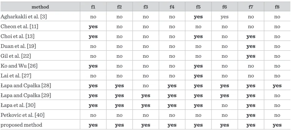
Table 1
The main properties of controller designing methods
method f1 f2 f3 f4 f5 f6 f7 f8
Agharkakli et al. [3] no no no no yes yes no no
Cheon et al. [11] yes no no no no no no no
Choi et al. [13] yes no no no yes no yes no
Duan et al. [19] no no no no no no yes no
Gil et al. [22] no no no no no no yes no
Ko and Wu [26] yes no no no yes no no no
Lai et al. [27] no no no no yes no no no
Łapa and Cpałka [28] yes yes no yes yes yes yes yes
Łapa and Cpałka [29] yes yes yes yes yes yes yes no
Łapa et al. [30] yes yes yes yes yes no yes no
Petkovic et al. [40] no no no no no no yes no
proposed method yes yes yes yes yes yes yes yes
f1 -Is a nature-inspired population-based algorithm used? f2 - Can the controller structure be dynamically selected?
unconventional applications, and it is usually done by the trial and error method. This demonstrates the GP’s advantage over the traditional methods. None-theless, the GP cannot be used directly for designing PID-based controllers, but it can be used for the selec-tion of a structure and parameters of tree structures (computer programs) that can be used as controllers. In order to create a specific type of a controller (e.g. a PIDC), the GP must be modified accordingly.
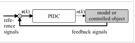
In paper [15], we considered a concept of a PIDC whose structure and parameters could be adjusted automatically using the proposed modification of the GP algorithm. The results obtained and presented in the paper were promising. In this paper, we also con-sider the problem of choosing the structure and tun-ing parameters of the PIDC (Fig. 2) on the basis of the model of a control object (Fig. 1). The control system considered in this paper (Fig. 1) works in three phases, i.e.: learning, testing, and verification. In the learning phase (which includes the selection of a structure and tuning parameters) a model of the con- trolled object is used. If a satisfactory PIDC is found in this phase (in terms of the assumed evaluation criteria), then the learning can be stopped. The PIDCs designed and optimized in the learning phase are then tested under conditions similar to those in the learning phase (the testing phase) and verified (the verification phase) under conditions other than those in the learning phase (including using a different test signal). After a positive completion of these phases (learning, test-ing and verification) an implementation on the target hardware platform can be done. The goal of the pro-posed approach is to choose a simple structure and parameters of the PIDC that meets the accepted eval-uation criteria for the problem under consideration. The elements of a novelty presented in this paper are as follows:
_ The PIDC structure includes a number of control blocks (CB, Fig. 3) (each composed of a few programmable switches and a single PID controller) and operation blocks (OP, Fig. 4) (each of them includes of a number of programmable switches and a single finite impulse response filter). The proposed genetic programming automatically tunes parameters of these PID controllers and filters (i.e. their order and cut-off frequency) as well as the states of their programmable switches. Such approach shows great possibilities of using genetic
programming combined with the genetic algorithm in the design of automatic control systems (both controllers and their supporting elements).
_ A new way of designing a PIDC structure: an aggregating operator (OP, Fig. 4) is introduced. Thus, we show that the GP algorithm can be very easily adapted to solve unusual optimization problems.
_ The way in which the population is processed by the GP algorithm is improved in comparison to [15]. In addition, the way in which the evolutionary operators are used to search the solution space is updated by introducing intensity of evolutionary operators. This shows that the GP is a flexible algorithm that can be extended by using unconventional evolutionary operators (often adjusted to the problem).
_ A new procedure of initial population initialization is proposed. We have specifically simplified the way of generating a population in comparison to [15]. _ A new way of aggregating of the components of
the evaluation function is applied. This method was introduced to evaluate the population of individuals in the evolutionary algorithm [29], but it has not been used yet when combined with the algorithm of genetic programming. Thus, we show that the GP algorithm can be easily adapted to solve practical problems in the field of multi-criteria (multi-objective) optimization.
The elements of novelty presented in this paper and those considered in the context of control theory and the problem of controller design have been included in Table 1.
The structure of this paper is as follows: in Section 2, the proposed structure is described. Section 3 pres-ents the proposed GP algorithm. Section 4 includes simulation results, and the conclusions are drawn in Section 5.
Figure 1
The control system (CS) considered in this paper
refe-rence
signals feedback signals
u k( ) e( )k
2. PIDC Structure and Its Encoding
for the GP Algorithm
In this paper a control system (CS, Fig. 1) based on a PIDC (Fig. 2) is considered. The PIDC structure had to be designed in such a way so that it could be selec-ted using the GP algorithm. Therefore, aggregating blocks (OP, Fig. 4) and control blocks (CB, Fig. 3) were separated. CBs are in practice single PID controllers. The OP+CB combinations called a node (see Fig. 2). Such approach shows that the way of aggregation of signals in the GP does not have to rely on basic ope-rators (e.g. basic mathematical opeope-rators), but it can be more complex and can have its own interpretation. 2.1. Control Blocks (CB)
The control blocks perform typical PID activities: proportional (P element, Fig. 3), integral (I element, Fig. 3) and differential (D element, Fig. 3) the in-put signal. The outin-put signal from the CB can be de-scribed as follows:
( )
(
)
( )
( )
( )
( )
(
)
(
)
CB CBCB CB CB
P P
CB 2
CB CB CB
CB
I I
2 0
CB CB CB CB
D D 1 , 2 1 k k k
C e k
C K e k
u k
C K e k
C
C K e k e k
= = − ⋅ + ⋅ ⋅ + = + ⋅ + ⋅ ⋅ + + ⋅ ⋅ − −
∑
(1)where eCB
( )
k stands for CB input signal (see Fig. 3);( )
CB
u k stands for CB output signal; CB P
K is the en-forcement parameter of P element; CB
I S / I
K =T T (TI stands for the integral time constant, and TS-for the control time step); CB
D D/ S
K =T T (TD stands for the dif-ferential time constant); CB
{ }
P 0,1
C ∈ decides on acti-vation of P term (P term is active if CB
P 1
C = , see Fig. 3);
{ }
CB
I 0,1
C ∈ decides on activation of I term; CDCB∈
{ }
0,1 decides on activation of D term; CCB∈{ }
0,1 decides on activation of the CB (CB is active if CCB=1, oth-erwise uCB( )
k =eCB( )
k , see Fig. 3). Parameters CBP K , CB
I K , CB
D K , CB
P C , CB
I C , CB
D
C , CCB are selected automat-ically by the GP algorithm.
2.2. Aggregation Blocks (OP)
OP blocks aggregate signals from CB blocks or control-ler input signals e
( )
k =e k0( )
, ,… e kl( )
, ,… en−1( )
k .Figure 2
The general structure of the PIDC controller considered in this paper blocks associated with signals -OP k e blocks associated with signals from CB -OP CB OP u k CB OP CB OP CB OP CB OP node leaf root node,N
The output signal of the OP blocks is defined as follows:
( )
( )
( )
(
)
( )
( )
(
)
( )
( )
(
)
( )
( )
(
)
( )
( )
( )
OP OP OP OP CBCB CB OP CB
L R
CB CB OP CB
L R
CB CB OP CB
L R
OP
CB CB OP CB
L R
OP OP FIL
FIL OP FIL
sgn
if 1and 0
if 1and 1
if 1and 2
if 1and 3
if 1and 0
if 1and 1
1
l l l l l l l l
o
u k u k l o
u k u k l o
u k u k l o
u k
u k u k l o
e k l C
e k l C
= = = = + = − = − = − = − + = − = = − − = − =
> − =
> − =
− = ( )
( )
( )
( )
( )
(
)
( )
CB OP OP OP OP 1.5 +1 CB2 L OP
%2 CB R FIL FIL FIL OP if 1 1 otherwise, 1 o l l l l
l l l l
u k l
u k
C e k
C e k
− = = = = ⋅ + = − + − ⋅ ⋅ + + − ⋅ (2) Figure 3
The structure of the control block (CB)
1 I P D CB P C CB I C CB D C CB C + + + + + P K K CB P K CB I CB D CB
e k uCB k
1
1
where lOP∈ −
{
1,0, ,… −n 1}
indicates the OPobjec-tive: it can be used for aggregation of signals OP
( )
L
u k
and OP
( )
R
u k from other CB (lOP= −1, see Fig. 4), or to attach the controller input signal e kl
( )
to PIDC(lOP> −1) (see Fig. 4), oOP decides on aggregation of OP
( )
L
u k and OP
( )
Ru k ( OP
( )
OP( )
L R
u k u+ k for oOP=0,
( )
( )
OP OP
L R
u k u− k for oOP=1, OP
( )
OP( )
L R
u k u k
− + for
OP 2
o = , and OP
( )
OP( )
L R
u k u k
− − for oOP =3); sgn
( )
⋅ stands for the signum function; % stands for the modulo operator; FIL( )
l
e k stands for input signal
( )
OP
l
e k after passing through the filter block; uOP
( )
k stands for the OP output signal; FIL{ }
0,1l
C ∈ stands for activation of the FIR for lOP> −1 (the filter is active if FIL 1
l
C = , otherwise OP
( )
OP( )
l
u k =e k ). The parame-ters lOP, oOP, and FIL 1
l
C = are selected automatically by the GP algorithm. Occurred in Eq. (2) and on Fig. 4 marks OP
( )
L
u k and OP
( )
Ru k are used to indicate these input signals of the OP block that come from child nodes (L-left, R-right) in case of lOP= −1.
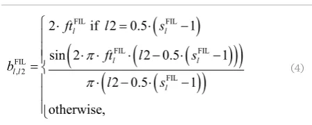
2.3. Filtration Blocks (FIL)
The filtration blocks (FIL, Fig. 4) are part of the OP blocks used to filter input signals of the PIDC. For the purpose of this paper finite impulse response (FIR) filters were used. FIRs are one of the most commonly used filters. The purpose of FIR filters is to smoothen signal values. It is achieved by averaging weighted val-ues from consecutive time steps. The output value of the filter depends on the filter length and its weights. Although FIR filters are used to improve the quality of control and to reduce impact of signal noise, they might decrease the controller efficiency if used incor-rectly [4, 45]. This is due to the fact that filtration adds a side-effect-phase delay of the filtered signal.
The output signal of the FIL can be described as fol-lows:
( )
FIL 1(
)
FIL FIL OP
, 2 2 0
2 ,
l
s
l l l l l
e k −b e k l
=
=
∑
⋅ − (3)where FIL
l
s stands for odd length of the filter (the filter has to have a middle element), OP
(
2)
l
e k l− stands for input signal l from k l− 2 time step, FIL
, 2
l l
b stands for the weight of the signal for k l− 2 time step calculated as follows [23]:
(
)
(
)
(
)
(
)
(
)
(
)
FIL FIL FIL FIL FIL , 2 FIL2 if 2 0.5 1
sin 2 2 0.5 1
2 0.5 1
otherwise,
l l l l l l
l
ft l s
ft l s
b l s π π ⋅ = ⋅ − ⋅ ⋅ ⋅ − ⋅ − = ⋅ − ⋅ − (4)
where FIL
l
ft stands for filter frequency. The parameters FIL
l
s and FIL
l
ft are selected automatically by the GP al-gorithm. It should be emphasized that Eq. (4) describes an exemplary form of FIL
, 2
l l
b , considered in [23]. The other approaches are described in e.g. [10, 17, 38, 44].
3. GP Algorithm Adjusted to the
Proposed PIDC Structure
The proposed GP algorithm can be used for the prob-lems where some structure and structure parameters have to be found (e.g. for problems that can be solved using a neural network or a fuzzy system). Therefore, it has a universal character. The idea presented in this paper combines the genetic algorithm (GA) (used for numeric parameter tuning) and genetic programming (GP) (used for parameter tuning and structure selec-tion). The combination of these methods required a change in the process of evolution and adaptation of the evolutionary operators used to search the space of the problem under consideration. This combination of the algorithms, however, has enabled an effective pop-ulation processing in which both integer (including bi-nary) and real parameters are used simultaneously.
OP L u k OP R u k + + + + OP %2 1o OP 1
sgn 1.5 +1
2
1 o
signals from other nodes
OP 0 e k FIL FIL 0 C + + + + 0 1 OP n-1
e k Cn-1FIL FIL + + 0 1
input signals FIL FIL-1, -1
n n s f
FIL, FIL
0 0 s f -1 0 n-1 OP l OP u k FIL 0 e k FIL n-1 e k Figure 4
The further part of this section describes: the struc-ture of an individual in the population(Section 3.1), an initialization of the population in the GP algorithm (Section 3.2), evolutionary operators used by the pro-posed GP algorithm (Section 3.3), a description of the idea of the proposed algorithm (Section 3.4) and a me-thod of evaluation of the individuals in the population (Section 3.5).
3.1. The Structure of an Individual in the Population
Each individual of population Xch is encoded in the form of the tree presented on Fig. 2:
CB CB CB
P I D
CB CB CB CB
P I D
OP OP FIL
OP OP
L R
FIL FIL
, , ,
, , , ,
{ } , , , ,
, ,
,
ch l
l l
K K K
C C C C l o C
u u s ft
= =
X N (5)
where N is the root of tree (Fig. 2), OP L
u and OP R u are references to child nodes (if they occur – see Fig. 2). Their structure is analogical to node N. A detailed in-terpretation of the parameters appearing in formula (5) is given in Sections 2.12.3.
The structure (length, complexity) of individual Xch of the proposed GP is therefore not predetermined, but it can be selected depending on the problem under consideration. It this paper, it is assumed that a tree height cannot be greater than TreeHeight (see Step 6 in Section 3.4).
3.2. Population Initialization
Initialization of each individual N proceeds as fol-lows:
Step 1. Creation of collection G containing elements of the tree (according to Figs 2-4). It consists of J
leaves (J is a parameter of the algorithm).
Step 2. Random assignment to each J element input signal e ki
( )
(i=0,1,...,n−1, where a positive valueindicates that a given element is a leaf) and the rest of the parameters (it takes into account the ranges of values of these parameters which depend on the problem under consideration, including filter param-eters).
Step 3. Selecting and removing from collection G
two randomly chosen elements of the tree. If they are associated with the same input signal (parameters
OP
l has the same value), then one of parameters lOP is changed randomly.
Step 4. Creating node (lOP= −1) that has the elements selected in Step 3 attached to it. The other parameters of the node are initialized randomly as described in Step 2.
Step 5. Putting the node created in Step 4 in collec-tion G.
Step 6. If collection G contains two or more ele-ments, go back to Step 3; otherwise go to Step 7. Step 7. Selecting from collection G the last node, and marking it as the root of the tree.
Step 8. Marking the root of the tree (with all nodes and leaves) as a single individual.
The initialization procedure should be repeated for all individuals of the GP population. The created pop-ulation is then processed according to the procedure described in Section 3.4.
3.3. GP Evolutionary Operators
The GP algorithm is dedicated to the PIDC process-ing and it combines the GA and GP evolutionary op-erators that have been additionally adjusted to the specification of the problem under consideration. It includes the following operators:
Tuning. This operator processes the real number val-ues of the PIDC ( CB
P K , CB
I K , CB
D K , FIL
l
s , FIL
l
f ). It works analogically to the GA mutation operator. If an as-sumption that vf stands for the vector of real num-ber values of the PIDC is made, then, the elements of this vector are modified as follows:
(
)
(
)
tuning
: 1,1 ,
i i i i
vf =vf +α ⋅U − ⋅ vfMax vfMin− (6)
where αtuning∈
[ ]
0,1 is an algorithm parameter that stands for tuning intensity; U(
−1,1)
gener-ates a random number from the range of[
−1,1]
;,
i i
vfMin vfMax
stands for the ranges of number val-ues vfi. This operator modifies only these elements of vf for which condition U(0,1)< ptuning is met.
The parameter ptuning∈
( )
0,1 of the GP algorithm iscalled tuning probability. Because the values gener-ated under Eq. (6) can go beyond the allowable range
,
i i
vfMin vfMax
out the repair procedure described in the next section (Step 6).
Mutation. This operator processes the integer pa-rameters ( CB
P C , CB
I C , CB
D
C , CCB, lOP, oOP, FIL
l
C ). If an assumption that vi stands for the vector of integer number values of the PIDC is made, then, the ele-ments of this vector are modified as follows:
(
)
: , ,
i i i
vi Ui viMin viMax= (7)
where Ui viMin viMax
(
i, i)
generates a random integernumber from the range of viMin viMaxi, i. The op-erator modifies only these elements of vi for which condition U(0,1)<pmutation is met. The parameter
( )
0,1mutation
p ∈ of the GP algorithm is called mutation probability.
Insertion. This operator selects randomly one node or leaf of the tree (excluding the root node) and replaces it with the root of a new randomly generated tree. The new tree is generated according to the procedure de-scribed in Section 3.2 on collection of Jinsertion leaves, where Jinsertion<J. Due to that, the tree does not grow significantly. The insertion is done only if condition:
(0,1) insert
U < p is met. The parameter pinsert∈
( )
0,1 ofthe GP algorithm is called insertion probability.
Pruning. This operator selects randomly one node of the tree (excluding the root node) and replaces it with a randomly generated leaf (lOP is set randomly to a value from the range of
[
0,n−1]
). The pruning iscarried out only if condition U(0,1)< ppruning is met.
Parameter ppruning∈
( )
0,1 of the GP algorithm is calledpruning probability.
Crossover. This operator works on the basis of two PIDCs. From each of them a random node (except the root node) is selected, and the nodes are swapped. The crossover is done only if condition U(0,1)< pcrossover is
met. Parameter pcrossover∈
( )
0,1 of the GP algorithm iscalled crossover probability.
3.4. Description of the Proposed GP Algorithm
The GP algorithm is based on a typical schema of a population-based algorithm (see e.g. [2, 42, 43, 49]). It uses two populations, i.e. the main one-P and an additional one-P′ and works according to the follow-ing steps:
Step 1. Initialization of population P with Ninit
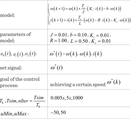
in-model: ( ) ( ) ( ( ) ( ))
( ) ( ) ( ( ) ( ) ( ))
1 1
s t
s
e T
k k K i k b k
J T
i k i k u k R i k K k
L
ω ω ω
ω
+ = + ⋅ ⋅ − ⋅
+ = + ⋅ − ⋅ − ⋅
parameters of
model: RJ==1.000.01, , bL==0.100.50, , KKte==0.010.01,
( )
0
e t , e t1( ),e t2( ): ω*
( )
t −ω( )
k , ω( )
k , i k( )
set signal: ω*( )t
goal of the control
process: achieving a certain speed ω*( )k
S
S
, , Tsim
T Tsim nIter T
= : 0.005 ,5 ,1000s s
,
uMin uMax: −50,50
Table 2
The description of the problem considered in the simulations
dividuals Xj (j=1,2, ,… Ninit) (see Section 3.2. Each individual encodes the whole structure and parame-ters of the PIDC.
Step 2. Evaluation of population P. Each individual is evaluated according to the criteria of the simula-tion problem. In the algorithm an assumpsimula-tion that the criteria are minimized is made. The evaluations are calculated on the basis of fitness function ff
( )
Xj (seeSection 3.5).
Step 3. Decreasing the size of P to Npop Ninit< by removing the individuals with worse fitness function values ff
( )
Xj .Step 4. Creating a copy of population P marked as P′. Step 5. Modification of population P′. In this step the following operations are performed: tuning, mutation, insertion, pruning, and crossover (see Section 3.3). Be-cause the crossover operator requires two individuals, the second one is drawn from population P.
Step 6. Repair of population P′. The repair proce-dure includes two types of actions. First of all, the values of the real parameters coded in the population are reduced to their permissible ranges. Second, the trees that are taller than TreeHeight are cut to the TreeHeight value (redundant nodes are turned into leaves). The TreeHeight is a parameter of the GP al-gorithm.
Step 8. Creation of a new population P. It combines best Npop individuals (according to the fitness func-tion) from populations P and P′.
Step 9. Correction of the intensity of the GP algo-rithm. This facilitates moving from exploration to exploitation of the search space and is implemented as follows:
{
}
{
}
{
}
{
}
{
}
: max ,
: max ,
: max ,
: max ,
: max , ,
tuning tuning tuning mutation mutation mutation insert insert insert pruning pruning pruning crossover crossover crossover
p pMin p
p pMin p
p pMin p
p pMin p
p pMin p
β β β
β β
= ⋅
= ⋅
= ⋅
= ⋅
= ⋅
(8)
where β∈
( )
0,1 is a reduction factor for the intensityof evolutionary operators.
Step 10. Checking the algorithm stop condition. If Table 3
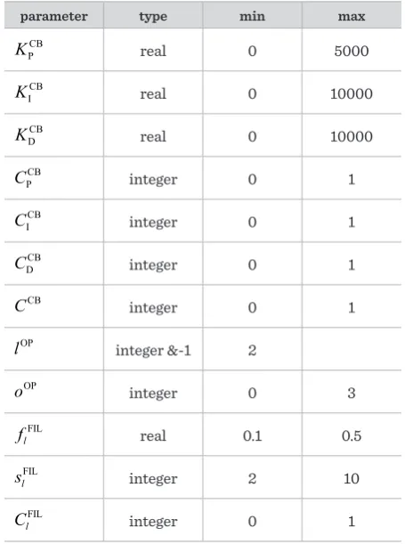
The ranges of PIDC parameters adopted in the simulations
parameter type min max
CB P
K real 0 5000
CB I
K real 0 10000
CB D
K real 0 10000
CB P
C integer 0 1
CB I
C integer 0 1
CB D
C integer 0 1
CB
C integer 0 1
OP
l integer &-1 2
OP
o integer 0 3
FIL
l
f real 0.1 0.5
FIL
l
s integer 2 10
FIL
l
C integer 0 1
Table 4
The values of the GP algorithm parameters adopted in the simulations (Nrepeats means the number of performed repetitions of each simulation)
parameter value
J [5, 12]
insertion
J [3, 7]
TreeHeight 5
Ninit 256
Npop 64
tuning
α 0.2
tuning
p 0.8
mutation
p 0.4
insert
p 0.2
pruning
p 0.4
crosover
p 0.9
β 0.990
tuning
pMin 0.025
mutation
pMin 0.050
insert
pMin 0.025
pruning
pMin 0.050
crosover
pMin 0.025
Nsteps 500
Nrepeats 40
the GP algorithm has performed a certain number of steps Nsteps (this is a parameter of the GP algo-rithm), then, the best individual from population P
is presented and the algorithm stops. Otherwise, the algorithm goes back to Step 4.
3.5. Evaluating Individuals
nFF. In this paper the criteria used for aggregation are normalized to the unit interval. The fitness func-tion is defined as follows:
( )
*( )
1
ff ,
ff sig ; ,
,
nFF
f ch ch f f
f f T w p q = = X X (9)
where fff
( )
Xch defines component f of fitnessfunc-tion (f =1,2, ,… nFF); wf∈
[ ]
0,1 stands forcompo-nent weights; sig
( )
⋅ stands for the function used for normalization of components to the range of[ ]
0,1;f
p , qf are normalization parameters; T*
{}
⋅ is thet-norm with weights of arguments used for aggrega-tion of the fitness funcaggrega-tion components.
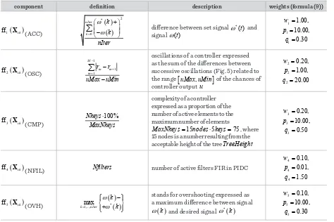
The components of ff (Xch) considered in this paper
are shown in Section 4 (including the parameters-see Table 5). The function used to normalize the compo-nents (sigmoid) is defined as follows:
component definition description weights (formula (9))
( )
1
ff Xch (ACC)
( )
( )
2 * 0 nIter k k k nIter ω ω = + − ∑
difference between set signal ω*( )t andsignal ω( )t
1 1 1 1.00, 10.00, 0.30 w p q = = =
( )
2ff Xch (OSC)
1 1 1
M
m m
m r r
uMax uMin − + = − −
∑
oscillations of a controller expressed as the sum of the differences between successive oscillations (Fig. 5) related to the range
[
uMax uMin,]
of the chances of controller output u2 2 2 0.20, 1.00, 20.00 w p q = = =
( )
3ff Xch (CMP)
100%
Nkeys MaxNkeys
⋅
complexity of a controller expressed as a proportion of the number of active elements to the maximum number of elements
15 5 75
MaxNkeys= nodes keys⋅ = , where 15 nodes is a number resulting from the acceptable height of the tree TreeHeight
3 3 3 0.20, 10.00, 0.50 w p q = = =
( )
4ff Xch (NFIL) Nfilters number of active filters FIR in PIDC
4 4 4 0.10, 0.01, 1.50 w p q = = =
( )
5ff Xch (OVH)
( )
( )
* 1,..., max k nIter k k ω ω = − + stands for overshooting expressed as a maximum difference between signal
( )
kω and desired signal ω*
( )
k5 5 5 0.10, 10.00, 0.30 w p q = = = Table 5
The evaluation criteria of fitness function ff ( )⋅ (nFF=5)
(
)
(
(
(
)
)
)
1sig , ,x p q = +1 exp p q x⋅ − − , (10)
where q is the center of the acceptable range
[
xMin xMax,]
of the changes of the domain of x pa-rameter (therefore sig , ,(
q p q)
=0.5)), and p is used to determine the angle of inclination of the central part of function graph sig( )
⋅ with respect to abscissa. The t-norm with weights of the arguments is defined as follows:{ }
{
(
)
}
(
(
)
)
*
1 1
; nFFf 1 f 1 f nFF 1 f 1 f ,
f
T T w a w a
= =
= − ⋅ − =
∏
− ⋅ −a w
(11)
where values wf ∈
[ ]
0,1 mean weights ofimpor-tance of the arguments af ∈
[ ]
0,1 . Please note that{
}
{
}
*
1, ;1,12 1, 2
T a a =T a a and *
{
}
1, ;1,02 1
Table 6
Averaged simulation results (each simulation variant was repeated Nrepeats=40 times)
variants ACC OSC CMP NFIL OVH ff
( )
⋅ N0+F0 0.0684 5.9756 0.1610 0.0000 0.0051 0.1449 N0+F1 0.0684 5.9748 0.1710 1.0250 0.0051 0.1457 N0+F2 0.0684 5.9729 0.1800 3.0000 0.0052 0.1467 N1+F0 0.0776 6.6790 0.1780 0.0000 0.0600 0.1561 N1+F1 0.0743 7.0941 0.1690 1.4250 0.0739 0.1541 N1+F2 0.0743 6.9947 0.1830 3.0000 0.0743 0.1554 N2+F0 0.0894 4.0407 0.1945 0.0000 0.1029 0.1706 N2+F1 0.0835 4.8588 0.1770 1.5250 0.0889 0.1634 N2+F2 0.0837 4.5800 0.1840 3.0000 0.0884 0.1643It is worth mentioning that other approaches for cri-teria aggregation might be also used. However, the approach expressed in formula (9) is simple to imple-ment and easy to expand. In addition, it allows one to give aggregated components a specific validity. This is a significant element for problems with multiple eva-luation criteria.
4. Simulation Results
Comments on the simulations carried out can be summarized as follows (Fig. 6, Fig. 7).
In the simulations a DC Motor (DCM) problem was considered [11]. This is a control problem in which the goal of the control is to achieve as fast as possible an angular velocity set by the motor shaft ω*.
A de-scription of this problem has been shown in Table 2. It is worth noting that the problem considered in the simulations can be seen from a practical point of view as an interesting benchmark in the optimization field.
Figure 5
The way of determining rm values for function ffOSC
( )
⋅ (seeTable 4)
t u( )t
0 r 1 r 2 r 3 r 4 r 5 r 6 r 7 r 8 Figure 6
Exemplary results obtained for the F1 simulation variant (filters selected dynamically) and different noise values: a) N0, b) N1, and c) N2. The dashed line indicates the set signal
Figure 7
Exemplary results obtained for the F1 simulation variant and verification set signal (different set signal than used in the learning and testing phases) and different noise values: a) N0, b) N1, and c) N2. The dashed line indicates the set signal
a)
t[s]
()
t
0 1 4 5
1.0 0.8 0.6 0.4 0.2 0.0 t[s] ut ()
0 1 4 5
50 30 10 -10 -30 -50 b) t [s] () t
0 1 4 5
1.0 0.8 0.6 0.4 0.2 0.0 t[s] ut ()
0 1 4 5
50 30 10 -10 -30 -50 c) t[s] () t
0 1 4 5
1.0 0.8 0.6 0.4 0.2 0.0 t[s] ut ()
0 1 4 5
50 30 10 -10 -30 -50 a) t[s] () t
0 1 4 5
1.2 1.0 0.8 0.6 0.4 0.2 0.0 t[s] ut ()
0 1 4 5
50 30 10 -10 -30 -50 b) t[s] () t
0 1 4 5
1.2 1.0 0.8 0.6 0.4 0.2 0.0 t[s] ut ()
0 1 4 5
50 30 10 -10 -30 -50 c) t[s] () t
0 1 4 5
1.2 1.0 0.8 0.6 0.4 0.2 0.0 t[s] ut ()
0 1 4 5
a)
CB
-+
u k
1
e k
0
e k
b)
CB
-u k
0
e k
2
e k
FIR 0.134
FIL 2
f
9
FIL 2
s
P 143.1
KCB
CB
P 546.7
KCB
c)
CB
+ +
u k
P 89.23
KCB
-0
e k
2
e k
FIR
9 0.324
FIL 2
f
FIL 2
s
1
e k
D 260.0
KCB
D 1626
KCB I
6188
KCB
D 1628
KCB
b)
t[s]
()
t
0 1 4 5
1.0 0.8 0.6 0.4 0.2 0.0
t[s]
ut
()
0 1 4 5
50 30 10 -10 -30 -50 c)
t[s]
()
t
0 1 4 5
1.0 0.8 0.6 0.4 0.2 0.0
t[s]
ut
()
0 1 4 5
50 30 10 -10 -30 -50 a)
t[s]
()
t
0 1 4 5
1.0 0.8 0.6 0.4 0.2 0.0
t[s]
ut
()
0 1 4 5
50 30 10 -10 -30 -50
_ The simulations were performed in different variants in which the assumed noise level of the signals measured from the object varied in the following ways: 0.0% (variant N0), 0.1% (variant N1), and 0.5% (variant N2). The aim of such an approach is to provide simulations with the conditions as close to the real conditions (prevailing in real CSs) as possible. In addition, variants of the PIDC structure, which differed in the way in which the filters were activated: filters not active (variant F0), dynamically activated filters (variant F1), filters active (variant F2) are taken into account.
_ In the simulations the GP algorithm was used, whose parameters are shown in Table 4. The purpose of this algorithm was to find the PIDC structure and parameters. The GP algorithm searched for parameter values considering the ranges shown in Table 3.
_ In the simulation the solutions (individuals of populations) were evaluated using fitness function
( )
ff ⋅ in the form of (9) with the criteria presented
in Table 4. The criteria taken into account include: control error, oscillations (the way in which they are calculated is shown in Fig. 5; it is worth pointing out that the noise is not included-little oscillations are not taken into account), complexity
Figure 8
The exemplary results obtained with taking only RMSE as the fitness function for the PIDC for the F1 simulation variant (wACC=1.0, wOSC=0.0, wCMP=0.0, wNFIL=0.0,
OVH 0.0
w = ) and different noise values: a) N0, b) N1, and c) N2. The dashed line indicates the set signal
and overshooting. In Table 4 the following additional markings were used: Nkeys that stands for the number of active keys ( CB
P C , CB
I C ,
CB D
C , CCB and FIL
l
C are treated as keys that allow for reduction of controller elements) in the CB and OP blocks; MaxNkeys is the number of active keys in the CB and OP blocks in the PIDC structure with the highest allowable TreeHeight value; Nfilters
is the number of active FIR filters in the PIDC structure. In Table 4 weights of criteria w and values of p, q used for criteria normalization by function (10) are given. The values of p and q
have been selected in such a way that the function (10) suits/covers in a best way the widest range of possible values of the corresponding criteria.
Figure 9
_ Each simulation variant has been repeated a certain number of times (Nrepeats=40), and the results were averaged (Table 6). Sample waveforms and the corresponding PIDCs structures are shown in Figs 6-9.
The conclusions from the performed simulations can be summed up as follows:
_ The results obtained in the simulations are satisfactory. The GP algorithm found a sufficient PIDC structure and parameters for the considered control problem in the sense of the adopted evaluation criteria.
_ Taking into account the noise of signals (N1 and N2 variants) coming from the object contributed to the activation of filters in F1 variants (Table 6, column NFIL; Fig. 9). For these variants, the best values of the evaluation function (positive) were obtained (Table 6, column ff
( )
⋅ )._ Activation of the filters slightly increased the
control accuracy in variants N1 and N2 (Table 6, column ACC). On the other hand, the activation of the filters in variants N0 (no noise) caused a slight increase in the value of the evaluation function (Table 6, column ff
( )
⋅ )._ In the simulations, an additional case was
considered when only the RMSE was taken into account in the evaluation function (wACC=1.0,
OSC 0.0
w = , wCMP =0.0, wNFIL=0.0, wOVH=0.0). This
resulted in a significant increase of oscillations of the control signal, increase in the value of the evaluation function, a reduction in overshooting (this phenomenon is beneficial), and only a slight increase in accuracy compared to the accuracy presented in Table 6. These results were considered as negative and are not included in this article. In Fig. 8 only an example of the result of such selected PIDC is presented.
_ PIDCs designed automatically by the GP work properly also for verification tests with the set signals other than those used in the learning phase (Fig. 7). This is an additional advantage of the approach proposed in this paper.
When comparing the results obtained in this paper with the results obtained by other authors, it is advis-able to take into account various assumptions made in the learning phase, various simulation variants and various methods of results presentation (e.g. showing
only the best achieved results). This comparison can be summarized as follows:
_ The authors in [1] used a different desired signal and the noise of the input signals has not been taken into account. The results obtained for them for neural network with 10 inputs (RMSE=0.4582) are worse than the results obtained in this paper (RMSE=0.1209). At the same time, the results obtained for a neural network with 15 input neurons (RMSE=0.0387) are better than the results obtained in this paper. It is worth noting that in paper [1] an identical testing and verifying set signal was used (in this work different set signals were used), which simplifies the problem under consideration.
_ The authors in [21] used a neural network sliding mode controller and took into account disturbance, load torque and uncertainties of the model with a purpose of improving the control process. The authors in [11] also considered a controller based on a neural network. The presented ideas of using neural networks are interesting, but the interpretation of their mode of operation is difficult. Neural network weights do not have their interpretation, unlike the P/I/D elements used in the PIDC.
_ The authors in [6] compared different controllers (PID-, state-space-, cascade ones) and obtained the settling time of the signal at the level of 0.6 s. The settling time for the PIDC selected by the GP was close to 0.35 s (see Fig. 7.a) and it was obtained for a more complex set signal (in [6] the set signal had a constant value). The authors in [34] also considered the problem of shortening the settling time. They proposed a hybrid-type controller: PID+ANN (artificial neural network) for which the obtained settling time was about 0.5 s.
for this controller (whose structure was, however, more complex than the PIDC’s) were therefore slightly better than those obtained in this paper (the accuracy of the FFPIDC without filters is equal to 0.0710, and accuracy of the PIDC without filters is equal to 0.0776-8.5% worse; the accuracy of the FFPIDC with filters is equal to 0.0690, and the accuracy of the PIDC with filters is equal to 0.0743-7.2% worse). It is worth noting, however, that the FFPIDC worked with about 3 times less overshooting compared to the PIDC (FFPIDC overshooting is about 0.37, and PIDC overshooting does not exceed 0.1).
_ It can be concluded that the solution proposed in this paper works with a good accuracy and it is characterized by simple implementation and a clear structure (this results from an unambiguous use of P/I/D). In addition, the obtained controllers were resistant to the noise of measuring signals and are able to function in changing operating conditions (see Fig. 7).
5. Conclusions
In this paper possibilities of using genetic program-ming (GP) for solving complex optimization prob-lems was shown. Such complexity results, among others, from the aim of the algorithm, which is selec-tion of structure and tuning parameters (in a typical approach only parameters of a fixed structure are tuned). Due to that the proposed GP has a universal character and can be used e.g. for designing of neu-ral network structures and their weights, selection of fuzzy system structures and tuning parameters of fuzzy rules, selection of evolutionary operators and
tuning their parameters, selection of a model and tun-ing its parameters, etc.
Moreover, this paper shows that the GP algorithm is a very flexible method. It allows for a simple adjust-ment of the algorithm, its operators and the method used for evaluating individuals to a given problem. What is more, a method of combining the GP with an-other algorithm, i.e. the genetic algorithm, has been presented. Thanks to that, the GP algorithm can effi-ciently process solutions with parameters encoded not only in real number values, but also in integral values. The solutions proposed in this paper have an interdis-ciplinary character, because they concern the theory of population algorithms and the control theory. The detailed purpose of these solutions is to support de-signers of controllers based on proven and almost per-fectly functioning PID controllers. We have proposed a new approach to designing of complex controllers built on the basis of PID controllers with the filtration of signals coming from the object. The purpose of the used filters with a finite impulse response is to improve the properties of those controllers (e.g. by elimination of controller output oscillations). This is particularly important when there is noise in measuring signals coming from a controlled object. The results obtained in the simulations were very satisfactory.
In the future, it is planned to use the proposed algo-rithm of genetic programming in other application areas related to complex adaptive systems. Moreover, hardware implementation of the proposed controllers and their testing in real control systems is also planned. Acknowledgments
The authors would like to thank the reviewers for their very helpful suggestions and comments in the revision process.
References
1. Aamir, M. On Replacing PID Controller with ANN Con-troller for DC Motor Position Control. International Journal of Research Studies in Computing, 2013, 2(1), 21-29. https://doi.org/10.5861/ijrsc.2013.236
2. Abdelbari, H., Shafi, K. Learning Structures of Con-ceptual Models from Observed Dynamics Using Evo-lutionary Echo State Networks. Journal of Artificial
Intelligence and Soft Computing Research, 2018, 8(2), 133-154. https://doi.org/10.1515/jaiscr-2018-0010 3. Agharkakli, A., Sabet, G. S., Barouz, A. Simulation and
4. Alia, M. A. K., Younes, T. M., Alsabbah, S. A. A Design of a PID Self-Tuning Controller Using LabVIEW. Journal of Software Engineering and Applications, 2011, 4, 161-171.https://doi.org/10.4236/jsea.2011.43018
5. Åström, K., Hägglund, T. Automatic Tuning of Simple Regulators with Specifications on Phase and Amplitude Margins. Automatica, 1984, 20(5), 645-651. https://doi. org/10.1016/0005-1098(84)90014-1
6. Baćac, N., Slukić, V., Puškarić, M., Štih, B., Kamenar, E., Zelenika, S. Comparison of Different DC Motor Po-sitioning Control Algorithms. Proceedings of the MI-PRO 2014, 2014, 26-30. https://doi.org/10.1109/MI-PRO.2014.6859832
7. Bansal, U. K., Narvey, R. Speed Control of DC Motor Using Fuzzy PID Controller. Advance in Electronic and Electric Engineering, 2013, 3(9), 1209-1220.
8. Bature, A. A., Muhammad, M., Abdullahi, A. M. Position Control of a DC Motor: An Experimental Comparative Assessment Between Fuzzy and State Feedback Con-troller. ARPN Journal of Engineering and Applied Sci-ences, 2013, 8(12), 984-987.
9. Caraveo, C., Valdez, F., Castillo, O. Optimization of Fuzzy Controller Design Using a New Bee Colony Al-gorithm with Fuzzy Dynamic Parameter Adaptation. Applied Soft Computing, 2016, 43, 131-142. https://doi. org/10.1016/j.asoc.2016.02.033
10. Chandra A., Chattopadhyay, S. Design of Hardware Effi-cient FIR FILTER: A REVIEW of the State-of-the-Art Approaches. Engineering Science and Technology, an International Journal, 2016, 19, 212-226.
11. Cheon, K., Kim, J., Haamadache, M., Lee, D. On Replacing PID Controller with Deep Learning Controller for DC Mo-tor System. Journal of Automation and Control Engineer-ing, 2015, 3(6). https://doi.org/10.12720/joace.3.6.452-456 12. Choi, H. H., Jung, J.-W. Discrete-Time Fuzzy Speed
Regulator Design for PM Synchronous Motor. IEEE Transactions on Industrial Electronics, 2013, 60(2), 600-607. https://doi.org/10.1109/TIE.2012.2205361 13. Choi, H. H., Yun, H. M., Kim, Y. Implementation of
Evo-lutionary Fuzzy PID Speed Controller for PM Synchro-nous Motor. IEEE Transactions on Industrial Infor-matics, 2015, 11(2), 540-547. https://doi.org/10.1109/ TII.2013.2284561
14. Cpałka, K. Design of Interpretable Fuzzy Systems. Spring-er, 2017. https://doi.org/10.1007/978-3-319-52881-6 15. Cpałka, K., Łapa, K., Przybył, A. A New Approach to
De-sign of Control Systems Using Genetic Programming.
Information Technology and Control, 2015, 44(4), 433-442. https://doi.org/10.5755/j01.itc.44.4.10214
16. Das, S., Pan, I., Das, S., Gupta, A. Genetic Algorithm Based Improved Sub-Optimal Model Reduction in Nyquist Plane for Optimal Tuning Rule Extraction of PID and Controllers via Genetic Programming. Proce-edings of the 2011 International Conference on Process Automation, Control and Computing, PACC 2011, 2011, 5978962. https://doi.org/10.1109/PACC.2011.5978962 17. Dinesh, P. S., Manikandan, M. Survey on
Reconfigu-rable Fir Filter Architecture. Proceedings of the 2017 Fourth International Conference on Signal Processing, Communication and Networking (ICSCN), Chennai, 2017, 1-3. https://doi.org/10.1109/ICSCN.2017.8085685 18. Do, T. D., Choi, H. H., Jung, J.-W. SDRE-Based Near
Optimal Control System Design for PM Synchronous Motor. IEEE Transactions on Industrial Electroni-cs, 2012, 59(11), 4063-4074.https://doi.org/10.1109/ TIE.2011.2174540
19. Duan, X. G., Deng, H., Li, H. X. A Saturation-Based Tun-ing Method for Fuzzy PID Controller. IEEE Transac-tions on Industrial Electronics, 2013, 60(11), 5177-5185. https://doi.org/10.1109/TIE.2012.2222858
20. El-Sousy, F. F. M. Intelligent Optimal Recurrent Wave-let Elman Neural Network Control System for Perma-nent-Magnet Synchronous Motor Servo Derive. IEEE Transactions on Industrial Informatics, 2013, 9(4), 1986-2003. https://doi.org/10.1109/TII.2012.2230638 21. Fallahi, M., Azadi, S. Adaptive Control of a DC Motor
Using Neural Network Sliding Mode Control. Proceed-ings of the International Multi Conference of Engineers and Computer Scientists (IMECS 2009), 2009, 2. 22. Gil, P., Lucena, C., Cardoso, A., Palma, L. B. Gain Tuning
of Fuzzy PID Controllers for MIMO Systems: A Perfor-mance-Driven Approach. IEEE Transactions on Fuzzy Systems, 2015, 23(4), 757-768. https://doi.org/10.1109/ TFUZZ.2014.2327990
23. Greensted, A. FIR Filters by Windowing. The Lab Book Pages: An Online Collection of Electronics Informa-tion, available online: http://www.labbookpages.co.uk/ audio/firWindowing.html, 2010.
24. Jezernik, K., Horvat, R., Curkovic, M. A Switching Control Strategy for the Reduction of Torque Ripple for PMSM. IEEE Transactions on Industrial Informatics, 2013, 9(3), 1272-1279. https://doi.org/10.1109/TII.2012.2222037 25. Kadlic, B., Sekaj, I., Pernecka, D. Design of
Programming. Proceedings of the 19th World Con-gress, The International Federation of Automatic Control Cape Town, South Africa, 2014. https://doi. org/10.3182/20140824-6-ZA-1003.00915
26. Ko, C. N., Wu, C. J. A PSO-Tuning Method for Design of Fuzzy PID Controllers. Journal of Vibration and Con-trol OnlineFirst, 2007, 14, 1-21.
27. Lai, J. G., Zhou, H., Hu, W. S. A New Adaptive Fuzzy PID Control Method and Its Application in FCBTM. Inter-national Journal of Computers Communications & Control, 2016, 11(3), 394-404. https://doi.org/10.15837/ ijccc.2016.3.753
28. Łapa, K., Cpałka, K. On the Application of a Hybrid Genetic-Firework Algorithm for Controllers Struc-ture and Parameters Selection. Advances in Intelligent Systems and Computing, Springer, 2016, 429, 111-123. https://doi.org/10.1007/978-3-319-28555-9_10
29. Łapa, K., Cpałka, K. Flexible Fuzzy PID Controller (FFPIDC) and a Nature-Inspired Method for Its Con-struction. IEEE Transactions on Industrial Infor-matics, 2018, 14, 1078-1088. https://doi.org/10.1109/ TII.2017.2771953
30. Łapa, K., Cpałka, K., Przybył, A., Saito, T. Fuzzy PID Controllers with FIR Filtering and a Method for Their Construction. LNCS, Springer, 2017, 10245, 761-772. https://doi.org/10.1007/978-3-319-59060-8_27
31. Łapa, K., Cpałka, K., Wang, L. New Method for Design of Fuzzy Systems for Nonlinear Modelling Using Different Criteria of Interpretability. LNCS, Springer, 2014, 8467, 212-227. https://doi.org/10.1007/978-3-319-07173-2_20 32. Lin, C.-K., Liu, T.-H., Yang, S.-H. Nonlinear Position
Con-troller Design with Input-Output Linearisation Tech-nique for an Interior Permanent Magnet Synchronous Motor Control System. IET Power Electronics, 2008, 1(1), 14-26. https://doi.org/10.1049/iet-pel:20070177 33. Liu, G., Chen, L., Zhao, W., Jiang, Y., Qu, L. Internal
Mod-el Control of Permanent Magnet Synchronized Motor Using SVM Generalized Inverse. IEEE Transactions on Industrial Informatics, 2013, 9(2), 890-898. https://doi. org/10.1109/TII.2012.2222652
34. Madheswaran, M., Muruganandam, M., Simulation and Implementation of PID-ANN Controller for Chop-per Fed Embedded PMDC Motor. ICTACT Journal on Soft Computing, 2012, 2(3), 319-324. https://doi. org/10.21917/ijsc.2012.0049
35. Maher, R. A., Mohamed, M. J., An Enhanced Genetic Pro-gramming Algorithm for Optimal Controller Design, In-telligent Control and Automation, vol. 4, pp. 94-101, 2013.
36. Malhotra, R., Sodh, R. Boiler Flow Control Using PID and Fuzzy Logic Controller. Proceedings of the IJCSET, 2011, 1(6), 315-31.
37. Morawiec, M. The Adaptive Backstepping Control of Permanent Magnet Synchronous Motor Supplied by Current Source Inverter. IEEE Transactions on In-dustrial Informatics, 2013, 9(2), 1047-1055. https://doi. org/10.1109/TII.2012.2223478
38. NagaJyothi, G., SriDevi, S. Distributed Arithmetic Ar-chitectures for FIR Filters-A Comparative Review. Proceedings of the 2017 International Conference on Wireless Communications, Signal Processing and Net-working (WiSPNET), Chennai, 2017, 2684-2690. 39. Perng, J.-W., Chen, G.-Y., Hsieh, S.-C. Optimal PID
Con-troller Design Based on PSO-RBFNN for Wind Tur-bine Systems. Energies, 2014, 7, 191-209. https://doi. org/10.3390/en7010191
40. Petkovic, D., Pavlovic, N. D., Cojbašic, Z., Pavlovic, N. T. Adaptive Neuro-Fuzzy Estimation of Underactu-ated Robotic Gripper Contact Forces. Expert Sys-tems with Applications, 2013, 40, 281-286. https://doi. org/10.1016/j.eswa.2012.07.076
41. Preindl, M., Bolognani, S. Model Predictive Direct Speed Control with Finite Control Set of PMSM Drive Systems. IEEE Transactions on Power Electronics, 2013, 28(2), 1007-1015. https://doi.org/10.1109/TPEL.2012.2204277 42. Rutkowski, L. Computational Intelligence, Springer,
2008. https://doi.org/10.1007/978-3-540-76288-1 43. Sadiqbatcha, S., Jafarzadeh, S., Ampatzidis, Y. Particle
Swarm Optimization for Solving a Class of Type-1 And Type-2 Fuzzy Nonlinear Equations. Journal of Artifi-cial Intelligence and Soft Computing Research, 2018, 8(2), 103-110. https://doi.org/10.1515/jaiscr-2018-0007 44. Sandhiya, V., Karthick, S., Valarmathy, M. A Survey of
New Reconfigurable Architectures for Implementing FIR Filters with Low Complexity. Proceedings of the 2014 International Conference on Computer Commu-nication and Informatics, Coimbatore, 2014, 1-9. https://doi.org/10.1109/ICCCI.2014.6921804
45. Segovia, R. V., Hsgglund, T., Astrom, K. J. Noise Filte-ring in PI and PID Control. Proceedings of the Ameri-can Control Conference, 2013, 1763-1770. https://doi. org/10.1109/ACC.2013.6580091
47. Szczypta, J., Przybył, A., Cpałka, K. Some Aspects of Evolutionary Designing Optimal Controllers. Artifici-al Intelligence and Soft Computing. LNCS, Springer, 2013, 7895, 91-100.
48. Tai, K., El-Sayed, A. R., Biglarbegian, M., Gonzalez, C. I., Castillo, O., Mahmud, S. Review of Recent Type-2 Fuzzy Controller Applications. Algorithms, 2016, 9(2). https:// doi.org/10.3390/a9020039
49. Tambouratzis, G. Using Particle Swarm Optimization to Accurately Identify Syntactic Phrases in Free Text. Journal of Artificial Intelligence and Soft Computing
Research, 2018, 8(1), 63-67. https://doi.org/10.1515/ jaiscr-2018-0004
50. Tao, C. W., Taur, J. S., Chang, Y. H., Chang, C. W. A Novel Fuzzy-Sliding and Fuzzy-Integral-Sliding Controller for the Twin-Rotor Multi-Input–Multi-Output System. IEEE Transactions on Fuzzy Systems, 2010, 18(5), 893-905. https://doi.org/10.1109/TFUZZ.2010.2051447 51. Yang, X.-S. Nature-Inspired Optimization Algorithms.
Elsevier, 2016.