ANALYSIS OF FLOW IN A CONCENTRIC ANNULUS USING FINITE ELEMENT
METHOD
I. D. Erhunmwun
1,*and M. H. Oladeinde
21,2 DEPARTMENT OF PRODUCTION ENGINEERING,UNIVERSITY OF BENIN,BENIN CITY,NIGERIA
E-mail addresses: 1[email protected], 2 [email protected]
ABSTRACT
This work presents the computational modelling of the velocity distribution of an incompressible fluid flowing in a cylindrical annulus pipe, using the finite element method. The result shows that the velocity distribution increases from the boundaries until midway between the boundaries where it was maximum. Also, the velocity increases as the viscosity decreases. The results obtained were compared with exact second order differential equation solution. The results obtained were highly accurate and converges fast to the exact solution as the number of elements increases.
Keywords: Concentric annulus, Finite element method, Viscosity, Pressure gradient, Exact solution.
1. INTRODUCTION
The flow of fluids is important for many engineering applications. Consequently, an understanding of the characteristics of fluid flow is of considerable interest in many areas of engineering and science [1]. Annular flow is a flow regime of two-phase gas-liquid. It is characterized by the presence of liquid fluid flowing on an annulus shaped channel. Annular flow is important in drilling and production in deviated and horizontal wells [2]. Concentric annular flows of fluids in pipes have had a number of engineering applications. Such as chemical mixing devices, bearings and in the drilling of oil wells [3]. The motion of fluid in a concentric annular pipe is governed by the Navier-Stokes equations. The fluid may be
compressible, slightly compressible or
incompressible.
The determination of an accurate characterization of fluid flow has been the subject of previous research. Some of these researchers include but not limited to Stokes, Reynolds, Navier, Bernoulli, Petroff and Summerfield. Their works formed the fundamental principles of fluid dynamics [4] and [5]. As a result of the complicated form of the Navier Stokes equation which governs fluid flow, researchers have resorted to numerical means for finding approximate solutions to them. Numerical computation of fluid flow through concentric annular has been considered by a number
of researchers. [6] used the finite difference method for simulation of thermal flow in a horizontal concentric annulus. Natural convection heat transfer in concentric horizontal annular containing a saturated porous media has been addressed by [7] using Galerkin’s technique. Finite volume technique was applied by [8] for the prediction of flows through concentric annulus with center body rotation. [9] used the finite element method to solve a problem on the velocity distribution in viscous incompressible fluid using the Lagrange interpolation function and compared their results with the exact differential equation solution. [10] used finite volume to analyse flow in a concentric annular tube having narrow gap. In this study, finite element method was used to analyse the distribution of velocity of a viscous
incompressible fluid flow using Lagrange
interpolation function in a cylindrical annulus pipe.
2. GOVERNING EQUATION
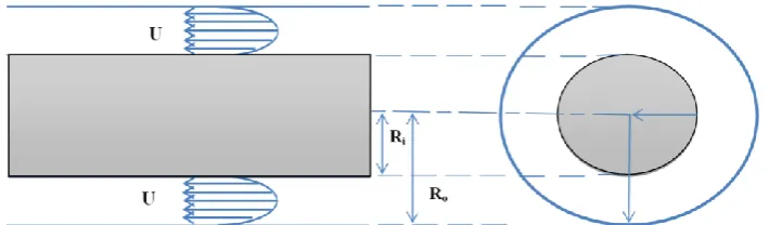
Consider the steady laminar flow of a Newtonian fluid with constant density in a long annular region between two coaxial cylinders of radii R0 and Ri as shown in Figure 1. The differential equation governing the velocity distribution is given by:
( )
( ) Copyright© Faculty of Engineering, University of Nigeria, Nsukka,
Print ISSN: 0331-8443, Electronic ISSN: 2467-8821
www.nijotech.com
Figure 1: Fluid flow between two coaxial cylinders
In (1), U is the velocity along the cylinder (i.e., the z component of velocity), µ is the viscosity, L is the length of the region along the cylinders in which the flow is fully developed, P1 and P2 are the pressures at z = 0 and z = L, respectively. P1 and P2 represent the combined effect of static pressure and gravitational force.
The boundary conditions are given by: r = Ri: U(r) = 0 and r = R0 : U(r) = 0.
2.1 Weak Formulation
Solving the strong form of equation (1) is not always efficient. Hence we seek to obtain the weak form of the governing differential equation by multiplying equation (1) by the weighted function (w) and integrating the final equation over the domain, we obtain
∫ ∫ ∫ [ (
) ]
( )
In equation (2)
f
0is given by known as the velocity gradient. Integrating equation (2) with respect to and and then incorporating the boundary conditions, we obtain∫ [
(
) ] ( )
∫
∫
( )
For an arbitrary degree of interpolation function given by equation (6)
( ) ∑
( ) ( )
And assuming that , equation (5) becomes
∑
∫
∫
( )
Equation (7) can be transformed into matrix form as: ⌊ ⌋ { } { } ( ) Where
∫
∫
∑
The Lagrange interpolation functions are given by equations (9) – (11).
( ) ( )( ) ( )
( ) ( )( ) ( )
(
)
( )
But in which, is a constant since the viscosity and velocity profile are constants in the fully developed region ( ) ( ) Integrate eq. 15 with respect to r, we have,
( ) Integrating eq. 19 again with respect to r, we have,
( )
ln ( ) At this time, we input the boundary conditions. The two boundary conditions may be evaluated by applying the boundary conditions of zero velocity at the inner and outer walls, i.e.,
r = Ri: U(r) = 0 r = R0 : U(r) = 0 After inputting the boundary conditions, we have that
ln( ) ( ) Therefore,
ln . Substitution of these values for the constants of integration into the equation yields the final expression for the velocity profile:
( )
[ ( )
( ) ln( ) ln (
r
)] ( )
3. NUMERICAL EXAMPLE
To illustrate the model and its accuracy, we consider the following example.
Consider a steady state laminar flow of a Newtonian fluid with constant density in a long annular region between two coaxial cylinders of radii Ri = 80 cm and R0 = 120 cm. Determine the velocity distribution for a
velocity gradient of 5N/m and fluid viscosity of µ = 0.75kgm/s, when the velocity at the end of the plates is zero.
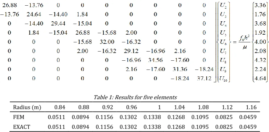
In other to solve this problem, a mesh of five uniform elements was used to represent the entire domain. The values of rA for the nth element is given by 0.8 + (n -1)h. The element matrices were obtained using equations (12) and (13). The stiffness matrices and the source vectors for the elements are shown below:
First Element [ ] [ . . . . . . . . . ] { } [ . . . ] Second element [ ] [ . . . . . . . . . ] { } [ . . . ] Third element [ ] [ . . . . . . . . . ] { } [ . . . ] Fourth Element [ ] [ . . . . . . . . . ] { } [ . . . ] Fifth Element [ ] [ . . . . . . . . . ] { } [ . . . ]
Imposing the boundary conditions which state that the velocity at the boundary is zero, we have:
Table 1: Results for five elements
Radius (m) 0.84 0.88 0.92 0.96 1 1.04 1.08 1.12 1.16
FEM 0.0511 0.0894 0.1156 0.1302 0.1338 0.1268 0.1095 0.0825 0.0459
EXACT 0.0511 0.0894 0.1156 0.1302 0.1338 0.1268 0.1095 0.0825 0.0459
In other to increase the accuracy, the same problem was analysed using ten elements. The results obtained along with the exact solution are shown in Figure 2. The behaviour of the error at the nodes was observed as the mesh was discretized further. In particular, nodal velocities for the flow regime and the associated error in relation to the exact were obtained for uniform meshes of 10 and 20 elements respectively. The progression of the nodal error is presented in Table 2.
The variation of the velocity profiles for different viscosities of fluid was obtained through a parametric study and presented in Figure 3.
Table 2: Comparison between percentage errors for different number of elements
Radius (m) Percentage Error (%)
5 elements 10 elements 20 elements 0.84 2.82 x10⁻³ 4.4965x10⁻⁶ 2.8163 x10⁻⁷
0.88 6.49 x10⁻⁵ 4.0863x10⁻⁶ 2.5592 x10⁻⁷
obtain nodal velocities for progressively finer mesh of 5, 10 and 20 elements respectively. The result of the numerical computation shows that the finite element solution converges towards the exact solution as the mesh becomes smaller. This deduction arose from an observation of the error at specific points on the domain of the problem as depicted in Table 2 for different mesh densities.
Parametric study was carried out to observe the evolution of the nodal velocities for different fluid viscosities. It is important to observe the velocity profiles for different viscosities as viscosity is temperature dependent.
Numerical computation put forward indicates that for very small values of the viscosity, the corresponding values of the velocities were very high. As the viscosity increases, the velocity decreases. This behaviour is attributable to fact that as the viscosity increases, the cohesive bond between the molecules of the fluid increase. When this happens, there will be reluctance for molecules of the fluid to slide. This therefore affects retards the velocity of the fluid. Thus, we can say that with all other conditions remaining constant, the viscosity and the velocity of a fluid are inversely related.
5. CONCLUSION
The finite element method has been used to obtain the velocity distribution of a fluid flowing in a cylindrical annulus pipe. Increased accuracy of the solution was obtained with mesh refinement. Parametric studies have indicated that the velocity of the fluid flow exhibits an inverse relationship with fluid viscosity for fluid flow in a cylindrical annulus pipe. Concentric annular flows of fluids in pipes have had a number of engineering applications such as chemical mixing devices, bearings and in the drilling of oil wells. This research has been able to provide the velocity distribution in the domain of a concentric annulus pipe at a glance with a very high accuracy compared to other methods that provides solution at a point.
6. REFERENCES
[1] Kim, Y. J, Han, S. M. and Woo, N. S. Flow of Newtonian and non-Newtonian fluids in a
concentric annulus with a rotating inner cylinder, Korea-Australia Rheology Journal, 25 (2) , pp 77-85, 2013.
[2] Ebrahim, N. H., El-Khatib, N. and Awang, M. Numerical Solution of Power-law Fluid Flow through Eccentric Annular Geometry, American Journal of Numerical Analysis, 2013, Vol. 1, No. 1, 1-7, 2013.
[3] Chunq, S. C. and Sung, H. J. Large-eddy simulation of turbulent flow in a concentric annulus with rotation of an inner cylinder” International Journal of Heat and Fluid Flow, vol. 26, 191–203, 2005.
[4] Fox, R. W. and McDonald, A. T. Introduction to Fluid Mechanics. John Wiley and Sons Inc., New York, 1996.
[5] Massey, B. and Wardsmith, J. Mechanics of Fluids. Nelson Thomas, United Kingdom, 2001.
[6] Shi, Y., Zhao, T. S., and Guo, Z. L. Finite difference-based lattice Boltzmann simulation of natural convection heat transfer in a horizontal concentric annulus, Comput. Fluids, 35, pp. 1–15, 2006.
[7] Alfahaid, A.F, Sakr, R.Y and Ahmed, M.I. Natural convection heat transfer in concentric horizontal annuli containing a saturated porous media, iium engineering journal, vol. 6, no. 1, pp 41-51, 2005.
[8] Naser J. A. “Prediction of Newtonian and Non Newtonian flow through concentric annulus with centre body rotation” International Conference on CFD IN Mineral and Material Processing and Power Generation, 1997.
[9] Akpobi J. A. and Akpobi E. D. A finite element analysis of the distribution velocity in viscous incompressible fluids using the Lagrange interpolation function. J. Appl. Sci. Environ. Manage, Vol. 11 (1) 31 – 38, 2007.