Learning Feed-Forward Control for a Two-Link
Rigid Robot Arm
Nguyen Duy Cuong
Electronics Faculty, Thai Nguyen University of Technology, Thai Nguyen City, Vietnam Email: [email protected]
Tran Xuan Minh
Electrical Faculty, Thai Nguyen University of Technology, Thai Nguyen City, Vietnam Email: [email protected]
Abstract—This paper introduces a control structure which consists of a Proportional Derivative (PD) controller and a Neural Network (NN)-based Learning Feed-Forward Controller (LFFC) to a Two-Link Rigid Robot Arm. An on-line B-spon-line neural network is used because of its local weight-updating characteristic, which has the advantages of fast convergence speed and low computation complexity. The torque applied to each link is defined using the Euler-Lagrange equation. The controller design takes into account the troubles caused by inertial loading, coupling reaction forces between joints, and gravity loading effects. This control structure can be directly applied to different robots within the same class with different lengths and masses. Simulation results are presented to demonstrate the robustness of our proposed controller under serve changes of the system parameters.
Index Terms—neural network (NN), learning feed-forward control (LFFC), two-link rigid robot arm
I. INTRODUCTION
Two-link manipulators are two-degree-of-freedom robots [1]. They are major components in the manufacturing industry due to their several advantages including speed, accuracy, and repeatability. However, control of two-link manipulators to track accurately a given trajectory is an extremely challenging due to the dynamics is highly non-linear and complex [1]. The inherent non-linear and complex behavior the two-link manipulator system makes it difficult to achieve high level performance and robustness simultaneously.
Proportional-Integral-Derivative (PID) control is the most common control algorithm used in industrial control systems [2]. However, a PID controller has some limitations. In order to cope with the fact that the parameters of the system being controlled are slowly time-varying and/or uncertain, and the presence of reproducible disturbances, high PID gains are required. However, having large gains can lead to system instability. In general, for the PID control design, a compromise has to be made between performance and robust stability.
Manuscript received April 15, 2014; revised July 16, 2014.
In order to eliminate positional inaccuracy due to reproducible disturbances and model uncertainty we consider a learning feed-forward controller structure that consists of a feedback and a feed-forward controller [3]. We assume that the state of the process and the state of the reference model are identical and use the approximated inverse dynamics of the process to compute the feed-forward signal. For proper reference signals and when there are no disturbances, if the feed-forward controller equals the inverse of the plant, the tracking error will be zero. The feed-back controller is designed such that robust stability is guaranteed in the presence of model uncertainty, while the feed-forward controller is used to compensate for known reproducible disturbances.
Neural network literature for function approximation is sufficiently wealthy. In its complete form, the problem involves both parametric and structural learning [4], [5]. The properties of a neural network are determined by its structure and the learning rule is used to adapt the weights. The network structure is defined based on the basic processing units and the way in which they are interconnected. The network allows any unit to be connected to any other unit in the network. The principal importance of a neural network is not only the way a neuron is implemented but also how interconnections are made. The learning rules, also known as training algorithms, are procedures for modifying the weights on the connection links in a neural network. Finding appropriate learning rules and finding an appropriate network structure are two different issues. Neural networks typically take a vector of input values and produce a vector of output values. Inside, the weights of neurons are trained to build a representation of a function that will approximate the input to output mapping [5].
This paper is organized as follows. Learning feed-forward control using B-spline neural network is introduced in Section II. In Section III, the dynamics of a two-link rigid robot arm is shown. The design of the proposed controller is introduced in Section IV. At the end of this paper, summary of the paper is given.
II. LEARNING FEED-FORWARD CONTROL USING B-SPLINE NEURAL NETWORK
A. Plant Disturbance Compensation
Motion control systems are usually designed to track given trajectories with small tracking errors. The assumed model of a plant with state dependent effects is illustrated in Fig. 1 [5].
Figure 1. Plant and reproducible disturbances.
There are only integrators in the forward path. The state dependent effects are assumed to be known and act on the input that generates effects which are known as reproducible disturbances. Thus, reproducible disturbances can be viewed as a function of the state of the plant. These disturbances may significantly affect the control performances during the object operations.
B. Learning Feed-Forward Control Using B-Spline Neural Network
Figure 2. Learning feed-forward control; A B-spline neural network is used in the feed-forward controller.
The control structure of combination between feedback controller and learning feed-forward controller using B-spline neural network is shown in Fig. 2. This adopts direct inverse control of B-spline neural network. The neural network inverse model of the plant is in series with the plant such that the transfer function between the input of the system and the output of the plant is equal to 1. In order to obtain the input-output behavior of an inverse dynamics model over time, the B-spline network should be trained. During training, the plant output is compared with a desired reference output. The error between these two signals is used to adjust the weights which are known as the free parameters of the function approximator [5].
( ) ∑ ( ) (1)
In which ( ) is the output of the BSN, ( ) is the membership of the basic function at input , the weight of the basis function, and is the number of B-splines. Training of the network can either be done after each sampling interval, which is known as on-line learning, or after a motion has been completed, known as off-line learning. In the on-line case, the cost function j that is minimized is the squared approximation error between the desired output of the BSN and the actual output :
( ) (2)
Applying the back propagation rule, this yields:
( ) (3)
Substituting (1) in (3) gives:
( ) ∑ ( )
( ) ( ) (4)
Figure 3. Top: I/O mapping; Bottom: order B-splines.
In this equation denotes the adaptation of the weight of the B-spline, and the learning rate
. In the off-line case the cost function is given by:
∑ ( ) (5)
+ + Plant
NL
+ +
Feedback
controller Plant
+
NL BSN – Function
approximator
-+ + + +
C. B-Spline Neural Network
The B-spline neural network (BSN) has become popular, mainly due to its ability to universally approximate any continuous nonlinear function [4], [5]. In a BSN the input-output mapping is created using basis functions, known as B-splines. A B-spline of order consists of piece-wise polynomial functions of order
(Fig. 3). The function evaluation of a B-spline is generally called the membership and is denoted as
where is the desired output for input and the actual output of the BSN. The adaptation of weights is then determined as:
∑ ( ) ( ) (6)
In order to prevent large weight-adaptations, (6) is normalized by:
∑ ( ) ( )
∑ ( ) (7)
The off-line learning rule (7) implies that the weights are updated after a reference motion has been completed.
D. Design of LFFC Using BSNs
In the detailed design of LFFC the following parameters of the feed-forward part have to be considered based on stability analysis in the frequency domain [5]:
1) Selection of the inputs of the feed-forward part The inputs of the BSN depend on the nature of the plant and the reproducible disturbances that the LFFC has to compensate. For random motions, the inputs should consist of the reference position and its derivatives/integrals.
2) Selection of the B-spline distribution on each of the inputs of the BSN
The BSN is able to accurately approximate a given signal by choosing a suitable width of the B-splines. A large number of “narrow” B-splines, allows the BSN to precisely approximate a high frequency signal. While a low frequency target signal requires a small number of “wide” B-splines.
3) The learning mechanism
Adaptation of the network weights can either be done after each sample, which is known as on-line learning, or after a motion has been completed, known as off-line learning.
4) The learning rate
The learning rate γ determines how strong the weights of the BSN are adjusted. A large learning rate implies that the weights are adjusted quickly. When a small learning rate is used the weights are adjusted slowly. However, a too high learning rate will cause un-stability.
By using a BSN, we have the following advantages: a. Local learning: Due to the compact support of the B-splines, only a small number of the weights contribute to the output. Only these weights need to be updated during training. While, in the case of the Multi-Layer Perceptron (MLP), during training all network weights need to be updated. This means, the BSN converges much faster than the MLP.
b. No local minima: The output of the BSN is a linear function of the weights. This implies that, both for off-line and on-off-line learning the learning mechanisms do not suffer from local minima. This means that the initial weights of the BSN do not influence the final tracking accuracy.
c. Tune-able precision: The choice of the number of the B-splines and their locations determines the smoothness of the input-output relation. Random target
signals can be accurately approximated, by choosing B-splines that have a proper compact support.
The principal drawback of BSNs is that the number of network weights grows exponentially with the dimension of the input space.
E. Input Selection of the LFFC
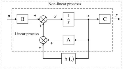
Models of the plant dynamics and of the reproducible disturbances are needed to create a structure for non-repetitive motions. We assume that the process can be modeled by a linear state space model and additive non-linear dynamics, shown in Fig. 4. This yields for the linear process
Figure 4. A linear process consists of a linear process a non-linearity ( )
̇ (8)
The state vector is chosen such that it consists of positions ( ) and their corresponding velocities ( ), ( ̇ ). This gives
[ ̇ ̇ ] [ ] [ ] [ ] (9)
Now we consider additive non-linear dynamics. For example, the case that the process has both a velocity and a position dependent non-linearity, this yields for the non-linear process:
[ ̇ ̇ ] [ ] [ ] [ ( ) ( )] [ ] (10)
The desired feed-forward signal , that makes the actual position of the process tracks the desired states , is given by (if exists):
( ̈
̇ ( )) (11)
The specific inputs of a BSN can be determined on the basis of a (non-linear) state space representation of the plant dynamics. To ensure the LFFC to accurately control the process for random motions, the states involved in (11) should be used as inputs of the BSNs. In general, this will result in a BSN that has multiple inputs. It is clear that when the disturbances depend on the velocity of the plant, the reference velocity must be used as input of the LFFC. In case the disturbances do not only depend on the velocity of the plant, but also on the acceleration, both the reference velocity and acceleration must be used as inputs of the LFFC. Each of the reference inputs of the LFFC will be used to compensate one specific disturbance [3].
+
+ +
A
B C
Non-linear processs
Linear process
III. DYNAMICS OF TWO-LINK RIGID ROBOT ARM
To determine the dynamics, examine Fig. 5, where we have assumed that the link masses are concentrated at the ends of the links.
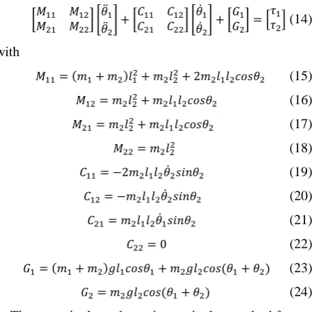
According to Lagrange’s equation, the arm dynamics are given by the two coupled non-linear differential equations [6], [7]:
[( ) ] ̈ (12)
[ ] ̈ ̇ ̇ ̇ ( ) ( ) [ ] ̈ ̈ (13)
̇ ( ) Figure 5. 2-DOF robot manipulator Writing the arm dynamics in vector form yields [ ] [ ̈ ̈] [ ] [ ̇ ̇] [ ] [ ] (14) with ( ) (15)
(16)
(17)
(18)
̇ (19)
̇ (20)
̇ (21)
(22)
( ) ( ) (23)
( ) (24)
These manipulator dynamics are in the standard form ( ) ̈ ( ̇) ̇ ( ) (25)
where is the vector of joint angels, ( ) is the inertia-matrix, ( ̇) describes Coriolis and centrifugal effects, ( ) models gravitational load and is the vector of joint motor torques. IV. DESIGN OF PROPOSED CONTROLLER A. Design the Reference Model Explicit position, velocity, and acceleration profile setpoint signals are created using the reference model, which is described by the transfer function [8], [9] ( ) (26)
The parameters of the reference model are chosen such that the higher order dynamics of the system will not be activated. The following numerical values are chosen: (27)
B. Design the Feedback Controller As discussed in the previous sections, tracking performance is obtained by the MRAS-based LFFC. The feedback controller is designed such that it features robust stability for closed loop when used alone. The compensator that is used is of the PD-type: ( ) (28)
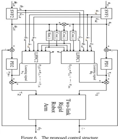
C. Determine the Inputs of the Feed-Forward Part The inputs of the Feed –Forward components depend on the nature of the plant and the reproducible disturbances that the LFFC has to compensate. For random motions, the inputs should consist of the reference position and its derivatives/integrals. We may conclude that the joint angels of a rigid robot manipulator can be controlled by mean of LFFC. The desired feed-forward signal is: ( ) ̈ ( ̇ ) ̇ ( ) (29)
A modified version of the feedback PD control law: ( ) ̈ ( ̇ ) ̇ ( ) ⏟ ⏟ ̇ (30)
where [ ], [ ], (31)
[ ] , [ ] , [ ], , , is the vector of desired joint angels, and is the vector of real joint angels. Substituting (13) in (31) yields the following desired feed-forward signals: [ ] [ ̈ ̈ ] [ ] [ ̇ ̇ ] [ ] [ ] [ ̇] [ ] [ ̇] [ ] (32)
From Eq. (12) and Eq. (13) we should select
[ ̇ ̇ ̈ ̈ ( ) ( ) ( )]as inputs of the feed-forward controller (see Table I and Fig. 6).
TABLE I. FEED-FORWARD COMPONENTS WITH CORRESPONDING
INPUTS AND THE TARGET FUNCTIONS THAT THEY HAVE TO
LEARN.
NO INPUTS LS TARGET FUNCTIONS
̈ [( ) ] ̈
̈ [ ] ̈
̇ ̇ ̇ ̇
̈ ̈
( )
( ) ( )
̈ [ ] ̈
̈ ̈
̇ ̇
( ) ( )
D. Choose the B-Spline Distribution
The aim of the BSN is to create the control signal that would result in the smallest possible tracking error. The width or support of the B-splines determines the accuracy such that the BSN is able to approximate an input-output relation. In case a one-dimensional BSN with second-order B-splines is used, the output consists of first-second-order polynomials between the B-spline knots. Therefore the smaller the distance between the B-spline knots the more accurate the LFFC can be obtained. When a small width is chosen the BSN is able to accurately approximate high frequency signals. Prior knowledge of the process and the disturbances are needed to determine the width of the B-splines. The minimum width of the B-splines for which the system remains stable, can be determined on the basis of a Bode plot of the negative complementary sensitivity function, | ( )| , of the closed loop. The following steps are given [3], [5]:
1. Determine | ( )| from a model of the closed loop system.
2. Use the Bode plot of the model to find out
{ | ( ) }| ( )| (33)
3. Search for the smallest value of at which
( ( )) satisfies
[ | ( )|
{ | ( ) }| ( )|
] (34)
4. The minimum value of the width of the B-splines, is given by
[ ] (35)
Because ( ) depends on the feed-back controller, it follows that if the obtained value is too large, the feedback controller should be redesigned.
E. Choose the Learning Rate
The learning rate determines how fast the weights of the BSN are adjusted. The larger the learning rate the
stronger weights can be updated, while a small learning rate implies that the weights are updated slowly. The learning rate is chosen relatively small, for example
. Also, a large means less attenuation of noise.
Figure 6. The proposed control structure
Simulation results
The parameter values of the considered two-link robotic arm are as follows: [ ] ;
[ ] ; [ ] ; [ ] ; ⁄ ;
[ ], [ ].
The desired tracking trajectories are supported to be: ( ) and ( ) for Link 1 and Link 2, respectively.
Figure 7. Comparison of the tracking error for theta_1 without (a) and with (b) LFFC.
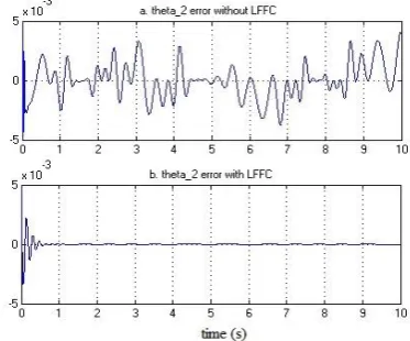
Fig. 7.a and Fig. 8.a show the tracking errors using the PD controllers only. The control system is clearly stable. However, the tracking performance is not satisfactory. Fig. 7.b and Fig. 8.b show the tracking errors when LFFC controllers are added. Non-linear signals are well compensated (see Fig. 9 and Fig. 10). Obviously, the combination between PD controller and Neural Network based Learning Feed-Forward controller indeed
SV
F1
PD
1
LF
FC
1
Tw
o-l
in
k
R
ig
id
R
ob
ot
A
rm
SV
F2
PD
2
C
os
(.)
Sin
(.)
C
os
(.)
+
-+ +
+
-+ +
+
LF
FC
2
Le
arn
in
g s
ig
na
l
Le
arn
in
g s
ig
na
l +
C
os
eliminates the tracking errors. In the beginning, the PD controller dominates. The LFFC controllers take less than haft second to learn and control the two – link robot motion very well.
Figure 8. Comparison of the tracking error for theta_2 without (a) and with (b) LFFC.
Figure 9. True non-linear signal ( ) (solid line) is well compensated by estimated signal (dashed line).
Figure 10. True non-linear coupling signal ̈ (solid line) is well compensated by estimated signal (dashed line).
V. CONCLUSION
The characteristics of the Learning Control introduced here are that the controller can be chosen as the inverse dynamical model of the plant and it is composed of the feed-forward loop besides the feedback controller loop. This type of learning control is known as the learning feed-forward control scheme. The feedback controller can be designed for robustness mainly, which does not require an accurate process model. The feed-forward controller compensates the reproducible disturbances that depend on the state of the process. Normally, a feed-forward controller is designed on the basis of an accurate process model of the process. The obtained LFFC does
not suffer from a trade-off between high performance and robust stability.
Nguyen Duy Cuong received the M.S. degree in Electrical Engineering from the Thai Nguyen University of Technology, Thai Nguyen city, Viet Nam, in 2001, the Ph.D. degree from the University of Twente, Enschede City, the Netherlands, in 2008.He is currently a lecturer with Electronics Faculty, Thai Nguyen University of Technology, Thai Nguyen City, Vietnam. His current research interests include real-time control, linear, parameter-varying systems, and applications in the industry. Dr. Nguyen DuyCuong has held visiting positions with the Universityat Buffalo- the State Universityof New York (USA) in 2009 and with the Oklahoma State University (USA) in 2012.
Tran Xuan Minh received the M.S. degree, and the Ph.D degree in Automation and Control Engineering from the Ha Noi University of Science and Technology, Viet Nam, in 1997 and in 2008, respectively. He is currently a lecturer with Electrical Faculty, Thai Nguyen University of Technology, Thai Nguyen City, Viet Nam. His current research interests include electronics Power, Process Control, and applications in the industry. Dr. Tran Xuan Minh has held visiting positions with the Oklahoma State University (USA) in 2013.
REFERENCE
[1] J. J. Craig,Introduction to Robotics, Mechanics and Control, 2nd Ed. Addison-Wesley, 1989.
[2] K. Ogata,Modern Control Engineering, Third Edition, Prentice Hall International, Simon and Schuster/A Viacom Company, Upper Saddle River, 1997.
[3] De Vries, J. A. Theo, L. J. Idema, and Velthuis, “Parsimonious Learning Feed-Forward Control,” European Symposium on Artificial Neural Networks ESANN, 1998.
[4] De Vries, J. A. Theo, Velthuis and L. J. Idema, “Application of Parsimonious Learning Feed-Forward Control to Mechatronic Systems,”IEE Pro. Control Theory Appl,Vol. 148, No. 4, July 2001.
[5] W. J. R. Velthuis, “Learning Feed-Forward Control: Theory, Design, and Applications,” PhD thesis, University of Twente, Enschede, The Netherlands, 2000.
[6] G. R. Yu and L. W. Huang, “Design of LMI-Based Fuzzy Controller for Two-link Robot Arm using Genetic Algorithms,” in Proc. of 2008 CACS International Automatic Control Conference National Cheng Kung University, Tainan, Taiwan, Nov. 21-23, 2008.
[7] R. Burkan, “Modeling of bound estimation laws and robust controllers for robustness to parametric uncertainty for control of robot manipulators”, Journal of Intelligent and Robotic Systems, Vol. 60, pp. 365–394, 2011.
[8] N. D. Cuong, T. J. A. De Vries, and J. Van Amerongen, “Application of NN-based and MRAS-based FFC to electromechanical motion systems,” in Proc. EPE’13 ECCE Europe 15th European Conference on Power Electronics and Application, 2013, pp. 1-10.