Volume 2007, Article ID 74580,21pages doi:10.1155/2007/74580
Research Article
Principal Component Analysis in ECG Signal Processing
Francisco Castells,1Pablo Laguna,2Leif S ¨ornmo,3Andreas Bollmann,4and Jos ´e Millet Roig5
1Grupo de Investigaci´on en Bioingener´ıa, Electr´onica y Telemedicina, Departamento de Ingener´ıa Electr´onica,
Escuela Polit´ecnica Superior de Gand´ıa, Universidad Polit´ecnica de Valencia (UPV), Ctra. Nazaret-Oliva, 46730 Gand´ıa, Spain
2Communications Technology Group, Arag´on Institute of Engineering Research, University of Zaragoza,
50018 Zaragoza, Spain
3Signal Processing Group, Department of Electrical Engineering, Lund University, 22100 Lund, Sweden
4Department of Cardiology, Otto-von-Guericke-University Magdeburg, 39120 Magdeburg, Germany
5Grupo de Investigaci´on en Bioingener´ıa, Electr´onica y Telemedicina, Departamento de Ingener´ıa Electr´onica,
Universidad Polit´ecnica de Valencia, Cami de Vera, 46022 Valencia, Spain
Received 11 May 2006; Revised 20 November 2006; Accepted 20 November 2006
Recommended by William Allan Sandham
This paper reviews the current status of principal component analysis in the area of ECG signal processing. The fundamentals of PCA are briefly described and the relationship between PCA and Karhunen-Lo`eve transform is explained. Aspects on PCA related to data with temporal and spatial correlations are considered as adaptive estimation of principal components is. Several ECG appli-cations are reviewed where PCA techniques have been successfully employed, including data compression, ST-T segment analysis for the detection of myocardial ischemia and abnormalities in ventricular repolarization, extraction of atrial fibrillatory waves for detailed characterization of atrial fibrillation, and analysis of body surface potential maps.
Copyright © 2007 Francisco Castells et al. This is an open access article distributed under the Creative Commons Attribution License, which permits unrestricted use, distribution, and reproduction in any medium, provided the original work is properly cited.
1. INTRODUCTION
Principal component analysis (PCA) is a statistical technique whose purpose is to condense the information of a large set of correlated variables into a few variables (“principal compo-nents”), while not throwing overboard the variability present in the data set [1]. The principal components are derived as a linear combination of the variables of the data set, with weights chosen so that the principal components become mutually uncorrelated. Each component contains new infor-mation about the data set, and is ordered so that the first few components account for most of the variability. In signal processing applications, PCA is performed on a set of time samples rather than on a data set of variables. When the sig-nal is recurrent in nature, like the ECG sigsig-nal, the asig-nalysis is often based on samples extracted from the same segment location of different periods of the signal.
Signal processing is today found in virtually any system for ECG analysis, and has clearly demonstrated its impor-tance for achieving improved diagnosis of a wide variety of cardiac pathologies. Signal processing is employed to deal
with diverse issues in ECG analysis such as data compres-sion, beat detection and classification, noise reduction, sig-nal separation, and feature extraction. Principal component analysis has become an important tool for successfully ad-dressing many of these issues, and was first considered for the purpose of efficient storage retrieval of ECGs. Over the years, this issue has remained central as a research topic, al-though the driving force has gradually changed from hav-ing been tiny hard disks to become slow transmission links. Noise reduction may be closely related to data compression as reconstruction of the original signal usually involves a set of eigenvectors whose noise level is low, and thus the recon-structed signal becomes low noise; such reduction is, how-ever, mostly effective for noise with muscular origin. Classi-fication of waveform morphologies in arrhythmia monitor-ing is another early application of PCA, in which a subset of the principal components serves as features which are used to distinguish between normal sinus beats and abnormal wave-forms such as premature ventricular beats.
the purpose of tracking temporal changes due to myocardial ischemia. Historically, such tracking has been based on lo-cal measurements derived from the ST-T segment, however, such measurements are unreliable when the analyzed signal is noisy. With correlation as the fundamental signal process-ing operation, it has become clear that the use of principal components offer a more robust and global approach to the characterization of the ST-T segment. Signal separation dur-ing atrial fibrillation is another recent application of PCA, the specific challenge being to extract the atrial activity so that the characteristics of this common arrhythmia can be stud-ied without interference from ventricular activity. Such sep-aration is based on the fact that the two activities originate from different bioelectrical sources; separation may exploit temporal redundancy among successive heartbeats as well as spatial redundancy when multilead recordings are analyzed.
The purpose of the present paper is to provide an overview of PCA in ECG signal processing. Section 2 con-tains a brief description of PCA fundamentals and an expla-nation of the relationship between PCA and Karhunen-Lo`eve transform (KLT). The remaining sections of the paper are devoted to the use of PCA in ECG applications, and touch upon possibilities and limitations when applying this tech-nique. The present overview is confined to those particular applications where the output of PCA, or the KLT, is con-sidered, whereas applications involving general eigenanaly-sis of a data matrix are left out. The latter type of appli-cations include singular-value-decomposition-(SVD)-based techniques for ECG noise reduction and extraction of the fe-tal ECG [2–7]. Another such application is the measurement of repolarization heterogeneity in terms of T wave loop mor-phology, where the ratio between the two most significant eigenvalues has been incorrectly denoted as PCA ratio, see, for example, [8,9].
2. METHODS
Principal component analysis in ECG signal processing takes its starting point from the samples of a segment located in some suitable part of the heartbeat. The location within the beat differs from one application to another and may in-volve the entire heartbeat or a particular activity such as the P wave, the QRS complex, or the T wave. Before the samples of a segment can be extracted, however, a fiducial point must be determined so that the exact segment location within the beat can be defined. Information on the fiducial point is typ-ically provided by a QRS detector and, sometimes, in com-bination with a subsequent algorithm for wave delineation [10]. Accurate time alignment of the different segments is a key point in PCA, and special care must be taken when per-forming this step.
The signal segment of a beat is represented by the column vector
x= ⎡ ⎢ ⎢ ⎢ ⎢ ⎣
x(1)
x(2) .. .
x(N) ⎤ ⎥ ⎥ ⎥ ⎥
⎦, (1)
whereNis the number of samples of the segment. The seg-ment is often extracted from several successive beats, thus re-sulting in an ensemble of M beats. The entire ensemble is compactly represented by theN×Mdata matrix,
X=x1 x2 · · · xM . (2)
The beatsx1,. . .,xMcan be viewed asMobservations of the random processx. While this formulation suggests that all beats considered originate from one patient, the beats may alternatively originate from a set of patients depending on the purpose of the analysis.
2.1. Principal component analysis
The derivation of principal components is based on the as-sumption that the signal xis a zero-mean random process being characterized by the correlation Rx = E[xxT]. The principal components ofxresult from applying an orthonor-mal linear transformationΨ=[ψ1 ψ2 · · · ψN] tox,
w=ΨTx, (3)
so that the elements of the principal component vectorw = [w1 w2 · · · wN]Tbecome mutually uncorrelated. The first principal component is obtained as a scalar product w1 =
ψT
1x, where the vectorψ1 is chosen so that the variance of w1,
Ew2 1
=EψT
1xxTψ1
=ψT
1Rxψ1, (4)
is maximized subject to the constraint thatψT
1ψ1 = 1. The
maximal variance is obtained whenψ1is chosen as the nor-malized eigenvector corresponding to the largest eigenvalue ofRx, as denotedλ1; the resulting variance is
Ew2 1
=ψT
1Rxψ1=λ1ψT1ψ1=λ1. (5)
Subject to the constraint thatw1 and the second principal component w2 should be uncorrelated, w2 is obtained by choosingψ2as the eigenvector corresponding to the second largest eigenvalue of Rx, and so on until the variance of x is completely represented by w. Accordingly, to obtain the whole set ofNdifferent principal components, the eigenvec-tor equation forRxneeds to be solved,
RxΨ=ΨΛ, (6)
where Λ denotes a diagonal matrix with the eigenvalues
λ1,. . .,λN. SinceRx is rarely known in practice, theN×N sample correlation matrix, defined by
Rx=
1
MXX
T, (7)
than those associated to other components, the ensemble ex-hibits a low morphologic variability, whereas a slow fall-off of the principal component values indicates a large variabil-ity. In most applications, the main goal of PCA is to con-centrate the information ofxinto a subset of components, that is,w1,. . .,wK, whereK < N, while retaining the physi-ological information (note that typicallyM N, otherwise
K <min(N,M)). The choice ofKmay be guided by various statistical performance indices [1], of which one index is the degree of variationRK, reflecting how well the subset ofK principal components approximates the ensemble in energy terms,
RK=
K
k=1λk
N
k=1λk
. (8)
In practice, however,K is usually chosen so that the perfor-mance is clinically acceptable and that no vital signal infor-mation is lost.
The above derivation results in principal components that characterize intrabeat correlation. However, it is equally useful to define anM×Msample correlation matrix
R•x=
1
NX
TX, (9)
in order to characterize interbeat correlation. In this case, the principal components are computed for each samplenrather than for every beat as was done in (3),
w(n)=Ψ•Tx(n), (10)
where
x(n)= ⎡ ⎢ ⎢ ⎢ ⎢ ⎣
x1(n)
x2(n) .. .
xM(n)
⎤ ⎥ ⎥ ⎥ ⎥
⎦, (11)
andΨ•Tis the eigenvector matrix ofR•x.
Figure 1illustrates the properties of the two types of sam-ple correlation matrices in (7) and (9), respectively, by psenting the related eigenvalues and eigenvectors and the re-sulting principal components. The analyzed signal is a single-lead ECG which has been converted into a data matrixXso that each of its columns contains one beat, beginning just be-fore the P wave.
WhenM N, it is much faster to diagonalizeR•xthan
Rx. This property can be realized by premultiplying both sides of
XTXψ•
k=λkψ•k (12)
byX, thus yielding
XXTXψ•k=λkXψ•k. (13)
Hence,Xψ•k is an eigenvector ofRx and the eigenvectorψk can be obtained as
ψk=Xψ•k, (14)
requiring far less computations than when diagonalizingRx. From now on, the bullet (•) notation is discarded since it is obvious from the context which of the two correlation ma-trices is dealt with.
The above assumption ofx being a zero-mean process can hardly be considered valid when the beats x1,. . .,xM originate from one subject and have similar morphology. While it may be tempting to apply PCA on X once the mean beat has been subtracted from each xi, such an ap-proach would discard important information. The common approach is therefore to apply PCA directly onX, implying that the analysis no longer maximizes the variance in (4), but rather the energy.Figure 2illustrates PCA for the two-dimensional case (i.e.,N=2) when the mean is either unal-tered or subtracted.
2.2. Relationship to the Karhunen-Lo`eve transform
The KLT is derived as the optimum orthogonal transform for signal representation in terms of the minimum mean square error (MSE) [11,12]. Similar to PCA, it is assumed thatxis a random process characterized by the correlation matrixRx=
E[xxT]. The orthonormal linear transform ofx is obtained by
w=ΦTx, (15)
where the set of basis functions Φ = [ϕ1 ϕ2 · · · ϕN] is to be determined so thatxcan be accurately represented in the minimum MSE sense using a subset of functions and the KLT coefficientsw1,. . .,wK. Decomposingxinto a signal es-timatex, involving the firstK (< N) basis functions, and a truncation errorv,
x=Φw=x+v (16)
with
x=
K
k=1
wkϕk, (17)
v= N
k=K+1
wkϕk, (18)
the goal is to choose Φso that the truncation error E =
E[vTv] is minimized. It can be shown that the optimal set of basis functions is produced by the eigenvector equation forRx,
RxΦ=ΦΛ, (19)
where the columns ofΦcontain the eigenvectors ofRxand the corresponding eigenvaluesλ1,. . .,λNare contained in the diagonal matrixΛ. The MSE truncation errorEis given by
E= N
k=K+1
λk (20)
0 2 4 6 8 10 12 14 16 18 20 2
1.5 1 0.5 0 0.5 1
Timen(s)
Amplitude
(mV
)
(a)
0 0.5 1
−0.25 0 0.25 −0.25 0 0.25 −0.25 0 0.25 −0.25 0 0.25
Timen(s)
A
dimensional
units
Eigenvectors
Rx=(XXT)/M λ1=0.91698
λ2=0.055413
λ3=0.022836
λ4=0.002045
1 5 10 15 20
2 0 2 0 2 0 2 4
k
wk
(mV
)
Principal componentswk
intrabeat
From beat #1
From beat #2
From beat #3
(b)
1 5 10 15
0.5 0 0.5 0.5 0 0.5 0.5 0 0.5 0.5 0 0.5
Beat order
A
d
imen
sio
n
al
un
its
EigenvectorsR¯
x=(XTX)/N λ1=1
λ2=1.7872e-016
λ3=2.2974e-017
λ4=4.0666e-018
0 0.5 1
0 0 0 6 4 2 0 2
Timen(s) w4
(
n
)
w3
(
n
)
w2
(
n
)
w1
(
n
)(
m
V
)
Principal components
wk(n) interbeat
(c)
Figure1: Transform-based representation of an ECG signal (a) segmented to include the whole beat (vertical lines) and produce the data matrixX. The eigenvectors (apart from a DC level) and principal components are displayed forRxobtained as (b) the intrabeat correlation
matrix defined in (7), or (c) the interbeat correlation matrix defined in (9).
are chosen since the sum of the eigenvalues then reaches its minimum value. This choice leads to that the eigenvectors corresponding to theKlargest eigenvalues should be used as basis functions in (17) in order to achieve the optimal
1 0 1 2 3 4 1.5
1 0.5 0 0.5 1 1.5 2 2.5 3 3.5
x(1)
x
(2)
Ψ1
Ψ2
Ψ1
Ψ2
Figure2: Eigenvectorsψ1andψ2forN =2, representing the di-rections to which the data should be projected (transformed) in or-der to produce the principal components of the displayed data set. Eigenvectors with origin at [0 0] result from non-zero mean data, whereas eigenvectors with origin at the gravity center of the data re-sult from data when mean is subtracted; note that either variance or energy is maximized depending on the case considered.
2.3. Singular value decomposition
The eigenvectors associated with PCA or the KLT can also be determined directly from the data matrixXusing SVD, rather than fromRx. The SVD states that anN×Mmatrix can be decomposed as [13]
X=UΣVT, (21)
whereUis anN×Northonormal matrix whose columns are the left singular vectors, andVanM×Morthonormal ma-trix whose columns are the right singular vectors. The mama-trix
Σis anN×Mnonnegative diagonal matrix containing the singular valuesσ1,. . .,σN,
Σ= ⎡ ⎢ ⎢ ⎢ ⎢ ⎣
σ1 0 · · · 0 · · · 0 0 σ2 · · · 0 · · · 0
..
. ... . .. ... ... ... 0 0 · · · σN · · · 0
⎤ ⎥ ⎥ ⎥ ⎥
⎦, (22)
assuming thatN < M.
Using the SVD, the sample correlation matrixRxin (7) can be expressed in terms of U and a diagonal matrix Λ whose entries are the normalized and squared singular val-uesσ12/M,. . .,σM2/M,
Rx= 1
MXX
T= 1
MUΣV
TVΣTUT =UΛUT. (23)
Comparing (23) with (6) and (19), it is obvious that the eigenvectors associated with PCA and the KLT are obtained as the left singular vectors ofU, that is,Ψ=U, and the eigen-valuesλkasσk2/M. In a similar way, the right singular vectors ofVcontain information on interbeat correlation, since they are associated with the sample correlationRxin (9).
2.4. Multilead analysis
Since considerable correlation exists between different ECG leads, certain applications such as data compression of multi-lead ECGs can benefit from exploring intermulti-lead information rather than just processing one lead at a time. In this section, the single-lead ECG signal of (1) is extended to the multilead case by introducing the vectorxi,l, where the indicesiandl denote beat and lead numbers, respectively. TheN×Lmatrix
Dicontains allLleads of theith beat,
Di=
xi,1 xi,2 · · · xi,L . (24)
2.4.1. Lead piling
A straightforward approach to applying PCA/KLT on multi-lead ECGs is to pile up the multi-leadsxi,1,. . .,xi,Lof theith beat into anLN×1 vectorxi, defined by
xi=
⎡ ⎢ ⎢ ⎢ ⎢ ⎣
xi,1 xi,2
.. .
xi,L
⎤ ⎥ ⎥ ⎥ ⎥
⎦. (25)
The piling operation is illustrated in Figure 3 for the case withL=2. Once all beats have been piled up into a set ofM
vectors, the ensemble of beats is represented by theLN ×M
multilead data matrix
X=x1 x2 · · · xM . (26)
Accordingly,XreplacesXin the above calculations required for determining the eigenvectors of the sample correlation matrix. Once PCA/KLT has been performed on the piled vec-tor, the resulting eigenvectors are “depiled” so that the de-sired principal components/KLT coefficients can be deter-mined for each lead.
2.4.2. Lead correlation
In certain studies, the SVD is applied directly to the multilead data matrixDi, thus bypassing the above lead piling opera-tion. Similar to the single-lead case above, the related left sin-gular vectors ofUcontain temporal information, however, the right singular vectors ofV contain information on in-terlead correlation (note that this case resembles the above-mentioned situation where interbeat correlation was ana-lyzed, cf. (9)). Hence, by considering allLleads at a certain timen, represented with the vector
xi(n)=
⎡ ⎢ ⎢ ⎢ ⎢ ⎣
xi,1(n) xi,2(n)
.. .
xi,L(n)
⎤ ⎥ ⎥ ⎥ ⎥
0 1 2 Time (s)
Amplitude
(a)
0 1 2 3 4 5
Time (s)
A
m
plitude
x1,1 x1,2 x2,1 x2,2
x¼
1 x
¼ 2
(b)
Figure3: Concatenation of a two-lead ECG signal containing two beats. (a) Each beat of the two leads is piled up into (b) one single vector.
0.1 (s/div)
2(
m
V
/d
iv
)
x8(n)
x7(n)
x6(n)
x5(n)
x4(n)
x3(n)
x2(n)
x1(n)
(a) Original ECG
0.1 (s/div)
2(
m
V
/d
iv
)
w8(n)
w7(n)
w6(n)
w5(n)
w4(n)
w3(n)
w2(n)
w1(n)
(b) Transformed ECG
Figure4: (a) The standard 12-lead ECG (V1,. . .,V6,I, andIIfrom top to bottom) and (b) its KL transform, obtained using (28), which concentrates the signal energy to only three of the leads.
the PCA/KLT can be used to concentrate the information into fewer leads, using
wi(n)=VTxi(n), n=1,. . .,N. (28)
This lead-reducing transformation is illustrated byFigure 4
for the standard 12-lead ECG (only 8 leads are unique for this lead system). Using the samples of the displayed signal segment to estimateRx, it is evident that the energy of the
original leads is redistributed so that only 3 out of the 8 trans-formed leadswi(n) contain significant energy; the remain-ing leads mostly account for noise although small residues of ventricular activity can be observed.
2.4.3. Independent time-lead correlation
A major disadvantage with the lead piling is that the total number of computations amounts toO(N3L3) [14]. One
ap-proach to reduce complexity is to consider the following se-ries expansion of the data matrixD:
D= N
n=1
L
l=1
wn,lBn,l, (29)
reasonable to assume that the basis functions are separable and described by rank-one matrices,
Bn,l=tnsTl, (30)
where the time vectortnconstitutes thenth column of the
N×N matrix T, and the lead vectorsl constitutes thelth column of theL×LmatrixS; bothTandSare assumed to be full rank. Then, the series expansion in (29) can be expressed in matrix form as
D=TWST, (31)
whereWis anN×Lmatrix formed by the coefficientswn,l, determined fromDby
wn,l=tTnDsl. (32)
When the correlation function is separable such that
Exi,l1
n1xi,l2
n2=rtn1,n2rsl1,l2, (33)
the correlation matrix of the piled vectorxcan be expressed as a Kronecker product,
Rx=Rt⊗Rs, (34)
whereRtandRscharacterize the temporal and spatial corre-lations, respectively. It has been shown that the eigenvectors ofRxcan be computed as the outer product of the
eigenvec-tors ofRt andRs, respectively [15]; these two sets of eigen-vectors thus constitute the eigen-vectorstnandslwhich define the rank-one matricesBn,lin (30). The sample correlation ma-trices ofRsandRtare obtained by
Rs= 1
MN
M
i=1
N
n=1
xi(n)xi(n)T,
Rt= 1
ML
M
i=1
L
l=1 xi,lxiT,l,
(35)
respectively. With the assumption of a separable correla-tion funccorrela-tion, the computacorrela-tional complexity is reduced from
O(N3L3) toO(N3+L3).
2.5. Adaptive coefficient estimation
In certain applications, truncation of the series expansion intoKbasis functions, (cf. (17)), is employed for the purpose of improving the signal-to-noise ratio (SNR). Interestingly, the SNR can be further improved when the signal is recur-rent since the basis function representation can be combined with adaptive filtering techniques. Such techniques make it possible to track time-varying changes in beat morphology even at relatively low SNRs. The main approaches to adap-tive coefficient estimation are the following.
(i) the instantaneous least mean square (LMS) algo-rithm with deterministic reference input. The coefficients are adapted at every time instant, producing a vectorw(n) [16–
20];
(ii) the block LMS algorithm. The coefficients are adapt-ed only once for each beat “block,” producing a vectorwithat corresponds to theith beat [21].
Although the instantaneous LMS algorithm is the adap-tive technique that has received most attention in biomedical signal processing, the block LMS algorithm represents a nat-ural extension of the above series expansion truncation, and is therefore briefly considered below. This algorithm can be viewed as a marriage of single-beat analysis, relying on the inner product computation to obtain the KLT coefficients, and the conventional LMS algorithm. In addition, the block LMS algorithm offers certain theoretical advantages over the instantaneous LMS algorithm with respect to bias and excess MSE (i.e., the error due to fluctuations in coefficient adapta-tion that cause the minimum MSE to increase).
The derivation of the block LMS algorithm takes its start-ing point in the MSE criterion, defined by
Ewi−1=E
xi−Φswi−1 T
xi−Φswi−1 , (36)
where the basis function matrixΦhas been partitioned into signal and noise subspaces,
Φ=Φs Φv . (37)
The block LMS algorithm iteratively finds the coefficient vec-tor by making use of the steepest descent algorithm [21],
wi=wi−1−1
2μ∇wi−1Ewi−1, (38) whereμdenotes the step size. Following substitution of the gradient expression and replacement of the expected value with its instantaneous estimate, the block LMS algorithm is given by
wi=(1−μ)wi−1+μΦTsxi. (39)
The algorithm is initialized byw0 =0which seems to be a
natural choice since, apart fromμ, it leads to the estimator of w1, that is,w1 = μΦTsx1. However, initialization to the inner product of the first beat, that is,w0 =ΦT
sx1, reduces the initial convergence time sincew1=ΦT
sx1[23]. The block LMS algorithm remains stable for 0< μ <2.
The block LMS algorithm reduces to single-beat analysis whenμ=1, since (39) then becomes identical to (15). When a complete series expansion is considered, that is,K=N, the block LMS algorithm becomes identical to conventional ex-ponential averaging. However, for the case of most practical interest, that is,K < N, the block LMS algorithm performs exponential averaging of the coefficient vector: an operation which produces a less noisy estimate of the coefficient vector, but also less capable of tracking dynamic signal changes.
For the steady-state condition whenxiis composed of a fixed signal componentsand a time-varying noise compo-nentvi, the block LMS algorithm can, in contrast to the in-stantaneous LMS algorithm, be shown to produce a steady-state coefficient vectorw∞which is an unbiased estimate of
2 1.5 1 0.5 0 0.5 1 1.5 2 2
1.5 1 0.5 0 0.5 1 1.5 2
x(1)
x
(2)
(a)
400 200 0 200 400
100 50 0 50 100 150 200
w1(arbitrary units)
w2
(ar
b
it
ra
ry
units)
Polynominal order 8
(b)
Figure5: (a) Plot of the two-sample datax(1) andx(2) generated by the hidden factorφ, see text, with Gaussian white noise added. The straight line represents the first eigenvector that results from PCA, whereas the circle represents the parametric curve that results from nonlinear PCA. It is clear that the projection error on the straight line is much larger than on the elliptic curve, and therefore nonlinear PCA has a superior concentration capability in this particular example. (b) An example of a nonlinear function (polynomial) capturing the dependency between the two largest principal components. (Reprinted from [22] with permission.)
of the block LMS algorithm is that its excess MSE is given by
Eex(∞)= μK
(2−μ)Nσ 2
v, (40)
whereσ2
v denotes the variance of the noise component. This expression does not involve any term due to the truncation error as does the excess MSE for the instantaneous LMS al-gorithm, and therefore, the block LMS algorithm is always associated with a lower excess MSE [10]. This property be-comes particularly advantageous when the signal energy is concentrated to a few basis functions.
2.6. Nonlinear principal component analysis
In certain situations, it is possible to further concentrate the variance of the principal components using a nonlinear transformation, making the signal representation even more compact than with linear PCA. This property can be illus-trated by the two-sample data vectorx = [x(1) x(2)]T = [cos(φ) sin(φ)]T, being completely defined by the uniformly distributed angle φ [24]. Applying PCA to samples result-ing from different outcomes ofφ, it is evident that the first principal component does not approximate the data ade-quately, see Figure 5(a). The parametric curve determined by the “hidden” factorφ, nonlinearly related to the samples throughφ=h(x)=cos−1(x(1)), produces a much better
ap-proximation. It is evident fromFigure 5(a)that the use ofφ
contributes to a lower error since the error between the ellip-soid and the data is much smaller than the error with respect to the straight line. Using ECG data,Figure 5(b)presents an example in which a nonlinear function (polynomial) cap-tures the relations between the two largest principal com-ponents. In this case, the nonlinear, polynomial, relation is shown in the PCA domain rather than in the data domain,
but equivalent relations could be displayed in the data do-main.
In general, it is assumed that the signalx =[x(1) · · ·
x(N)]Tis generated by some underlying feature vectorφ= [φ1 · · · φK]T, K ≤ N, throughN nonlinear continuous decoding functions fromRKtoR,x(1)=g1(φ),. . .,x(N)=
gN(φ), which have the inverse coding functions from RN to R, φ1 = h1(x),. . .,φK = hK(x). The coding function
h=[h1 · · · hK]T fromRNtoRKand the decoding func-tion g = [g1 · · · gN]T fromRK to RN are members of some setsFcandFdof nonlinear functions, respectively. The goal of nonlinear PCA (NLPCA) is to minimize the nonlin-ear reconstruction mean square error
ε=Ex−gh(x)2 (41)
for an optimum choice ofgandhin the setsFcandFd, re-spectively. The solution will depend on the choice ofFcand
Fdas well as the signalx. Linear PCA represents a particular case of NLPCA in which the two spaces are related to each other through linear mapping.
Unfortunately, there are in general an infinite number of solutions to the NLPCA minimization problem so that the hidden parameters are not unique. In fact, if a pair of func-tions,h1(·) andg1(·), achieves the minimum error, so does any pairh1(q−1(·)),q(g1(·)) for any invertible functionq(·).
However, by keeping eithergorhfixed, a set can be deter-mined which gives a unique result [24,25]:
(i) the setFd = {l(φ) for allφ∈RK}of contoursl(φ)= {x:h(x)=φ}for the functionh;
(ii) the setFcis constituted by theK-parametric surface
C= {g(φ) for allφ∈RK}generated byg.
repre-sented by the surface curve from R1 to R2, that is, x = g(φ)=[cos(φ0) sin(φ0)]T.
3. DATA COMPRESSION
Since a wide range of clinical examinations involves ECG sig-nals, huge amounts of data are produced not only for im-mediate scrutiny, but also for database storage for future re-trieval and review. Although hard disk technology has un-dergone dramatic improvements in recent years, increased disk size is parallelled by the ever-increasing wish of physi-cians to store more information. In particular, the inclusion of additional ECG leads, the use of higher sampling rates and finer amplitude resolution, the inclusion of noncardiac sig-nals such as blood pressure and respiration, and so on, lead to rapidly increasing demands on disk size. An important driving force behind the development of methods for data compression is the transmission of ECG signals across pub-lic telephone networks, cellular networks, intrahospital net-works, and wireless communication systems. Transmission of uncompressed data is today too slow, making it incom-patible with real-time demands that often accompany many ECG applications.
3.1. Single-lead compression
Transform-based data compression assumes that a more compact signal representation exists than that of the time-domain samples which packs the energy into a few coeffi -cientsw1,. . .,wK. TheseKcoefficients are retained for stor-age or transmission while the remaining coefficients are dis-carded as they are near zero. Transform-based compression is usually lossy since the reconstructed signal is allowed to differ from the original signal, that is, the truncation errorv
is not retained. Although a certain amount of distortion can be accepted in the reconstructed signal, it is absolutely essen-tial that the distortion remains small enough in order not to alter the diagnostic content of the ECG. Several different sets of basis functions have been investigated for ECG compres-sion purposes, and the KLT is one of the most popular as it minimizes the MSE of approximation [26–32].
Transform-based compression requires that the ECG first be partitioned into a series of successive blocks, where each block is subjected to data compression. The signal may be partitioned so that each block contains one beat. Each block is positioned around the QRS complex, starting at a fixed dis-tance before the QRS, including the P wave and extending be-yond the end of the T wave to the beginning of the next beat. Since the heart rate varies, the distance by which the block extends after the QRS complex is adapted to the prevailing heart rate. Hence, the resulting blocks vary in length, intro-ducing a potential problem in transform-based compression where a fixed block length is assumed. This problem may be solved by padding too short blocks with a suitable sample value, whereas too long blocks can be truncated to the de-sired length. The use of variable block lengths has been stud-ied in detail in [33,34]; the results show that variable block lengths produce better compression performance than fixed
blocks. It should be noted that partitioning of the ECG is bound to fail when certain chaotic arrhythmias are encoun-tered such as ventricular fibrillation during which no QRS complexes are present.
A fixed number of KL basis functions are often consid-ered for data compression, where the choice of K may be based on considerations related to overall performance ex-pressed in terms of compression ratio and reconstruction er-ror. The performance of the KLT can be described by the indexRk, defined in (8), which reflects how well the origi-nal sigorigi-nal is approximated by the basis functions. While this index describes the performance on the chosen ensemble of data as an average, it does not provide information on the reconstruction error in individual beats. Therefore, it may be appropriate to include a criterion for quality control when
K is chosen. Since the loss of morphologic detail causes in-correct interpretation of the ECG, the choice of K can be adapted for every beat to the properties of the reconstruction error (x−x), where the estimatexis determined from theK
most significant basis function [32], (cf. (17)). The value ofK
may be chosen such that the root mean square (RMS) value of the reconstruction error does not exceed the error toler-ance ε, whereas a more demanding approach is to choose
K such that none of the reconstruction errors of the entire block exceedsε. Yet another approach to the choice ofKmay be to employ an “analysis-by-synthesis” algorithm which is designed to ensure that the errors in ECG amplitudes and durations do not become clinically unacceptable [35,36].
By lettingK be variable, one can fully control the qual-ity of the reconstructed signal, however, one is also forced to increase the amount of side information since the value ofK
must be stored for every data block. If the basis functions are a priori unknown, a larger number of basis functions must also be part of the side information.Figure 6illustrates sig-nal reconstruction for a fixed number of basis functions and a number determined by an RMS-based quality control crite-rion. In this example, the indicated error tolerance is attained by using different numbers of basis functions for each of the three displayed beats.
The estimation ofRx can be based on different types of data sets. The basis functions are labeled “universal” when the data set originates from a large number of patients, and “subject-specific” when the data set originates from a single recording. While it is rarely necessary to store or transmit universal basis functions, subject-specific functions need to be part of the side information. Still, subject-specific basis functions offer superior energy concentration of the signal because these functions are better tailored to the data, pro-vided that the ECG contains few beat morphologies.Figure 7
illustrates the latter observation by presenting the recon-structed signal for both types of basis functions. One ap-proach to reduce the side information is to employ wavelet packets since these approximate to the KLT by efficiently cod-ing the basis functions [37].
0 1 2 3 4
2 0 2
Time (s)
A
m
plitude
(mV
)
K=6
ε=91μV
K=6
ε=109μV
K=6
ε=89μV Residual ECG
Original and reconstructed ECG using the KLT
(a)
0 1 2 3
4 2 0 2
Time (s)
A
m
plitude
(mV
)
K=18
ε=39μV
K=13
ε=38μV
K=17
ε=33μV Residual ECG
Original and reconstructed ECG using the KLT
(b)
Figure6: Quality control and KLT-based data compression. (a) A fixed number of basis functions (K=6) is used for signal reconstruction. (b) The number of basis functions is chosen so that the RMS error, denoted asε, between the original and reconstructed signals is always below 40μV. For ease of interpretation, the residual ECG is plotted with a displacement of−3 mV.
course of a stress test. Since the basis functions account for the T wave occurrence at a fixed distance from the QRS com-plex, the basis functions become ill-suited for representing beats whose T waves occur earlier or later than this interval. As a result, additional basis functions are required to achieve the desired reconstruction error, thus leading to less efficient compression. The representation efficiency can be improved by resampling of the ST-T segment in relation to the length of the preceding RR interval.
A nonlinear variant of PCA has also been considered for single-lead data compression, the goal being to exploit the nonlinear relationship between different principal com-ponents [22]. The method is based on the assumption that higher-order components can be estimated from knowledge of the firstkcomponents bywi=fi,k(w1,. . .,wk),i > k, with-out having to store the higher-order components (kwas set to 1 in [22]). Although the coefficients that define the nonlin-ear functions must be stored, their storage requires very few bytes. One way to model the nonlinear relationship is to use a polynomial with a small number of coefficients (typically 7 or 8), seeFigure 5(b).
3.2. Multilead compression
With transform-based methods, interlead correlation may be dealt with in two steps, namely, a transformation which concentrates the signal energy spread over the available L
leads into a few leads, followed by compression of each trans-formed lead using a single-lead technique. Following
con-centration of the signal energy using the transform in (28), different approaches to data compression may be applied to the transformed leads, of which the simplest one is to just retain those leads whose energy exceeds a certain limit. Each retained lead is then compressed using the above single-lead methods, or some other compression techniques. If a more faithful reconstruction of the ECG is required, leads with less energy can be retained, although they will be subjected to more drastic compression than the other leads [38].
A unified approach, which jointly deals with intersam-ple and interlead redundancy, is to pile all segmented leads
xi,1,. . .,xi,Linto a single vectorxi subjected to compression using any of the single-lead transform-based methods de-scribed above [29,39]. Applying the KLT, lead piling offers a more efficient signal representation than does the two-step approach, although the calculation of basis functions through diagonalization of theLN×LNcorrelation matrix is much more costly, in terms of computational measures, than for theL×Lmatrix in (9). However, when it is reasonable to assume that the time-lead correlation is separable, (cf. (30)), the computational load can be substantially reduced.
4. MYOCARDIAL ISCHEMIA
0 0.5 1 1.5 2 2
1 0 1
Time (s)
A
m
plitude
(mV
)
Residual ECG Original and reconstructed ECG
0 1 2 3 4
Time (s)
KL
basis
function
λ2=0.247 λ4=0.046 λ6=0.024
λ1=0.465 λ3=0.08 λ5=0.039
0 10 20 30
2 0 2
k
wk
Universal KLT
(a)
0 0.5 1 1.5 2
2 1 0 1
Time (s)
A
m
plitude
(mV
)
Residual ECG Original and reconstructed ECG
0 1 2 3 4
Time (s)
KL
basis
function
λ2=0.052 λ4=0.002 λ6=0.0001
λ1=0.918 λ3=0.025 λ5=0.001
0 10 20 30
0 2 4
k
wk
Subject-specific KLT
(b)
Figure7: Transform-based data compression using the KL basis functions derived from either (a) a huge database including thousands of ECGs from different subjects or (b) subject-specific data. The basis functionsϕkand associated eigenvaluesλkare presented as are the 30
largest coefficients of the original ECG’s KLT. The ECGs are reconstructed withK=8 and 2 for universal and subject-specific basis functions, respectively. For ease of interpretation, the residual ECG is plotted with a displacement of−2 mV.
flow often causes chest pain or discomfort (angina pectoris), but can also be completely unrelated to chest pain (silent is-chemia). Ischemia is associated with electrical instability of the heart that may initiate life-threatening ventricular tach-yarrhythmias such as ventricular fibrillation.
Myocardial ischemia is usually manifested in the ECG as morphologic changes of the ST segment and T wave, jointly referred to as ST-T changes, but may also occur unnoticed. While the normal ST segment starts at the isoelectric line and curves smoothly upwards into the T wave, the ischemic ST segment is instead horizontal or slopes downwards and may start well below the isoelectric line. An ST segment which drops below the isoelectric line is referred to as an ST depres-sion. An ischemic T wave is often more flat than a normal T
wave and may exhibit biphasic morphology or negative po-larity.
1:20 5:00 5:20 5:33
0 2 4 6 8 10
100 50 0 50 100
Minutes
A
rbit
rar
y
u
nits w1(i)
Figure8: The series of the most significant KLT coefficientw1(i) obtained from a patient undergoing balloon inflation in a coronary artery. The four beats (upper panel) correspond to the times indi-cated by the arrows on thew1(i) series (lower panel). Note that the ST-T segment is initially positive, as reflected by positive values of
w1(i), but later changes polarity is inverted and exhibits consider-able variation in magnitude.
This method is illustrated by Figure 8, where the ischemic episode is well-reflected by the drastic changes that occur in the most significant KL coefficient. It has been shown that this method offers better performance, that is, higher sensi-tivity and specificity, than the classical indices [42].
Using a universal data set of 100 000 beats, it has been shown that four KLT coefficients are sufficient to represent 90% of the ST-T segment energy [34]. Before the correlation matrix of the data set is estimated, it is essential to remove baseline wander so as to not account for that unwanted ac-tivity in the analysis. Moreover, it may be necessary to “nor-malize” the ST-T segment with respect to heart rate to ob-tain more efficient signal representation; signals recorded at widely different heart rates should be resampled so that the ST-T segments become more comparable. The resampling strategy has been shown to improve the energy representa-tion by 5% when considering the first two KLT coefficients [34].
Although the estimation of KLT coefficients can be done with (15), it is suitable to use adaptive techniques, (cf. (39)), to better cope with noise when the ECG is recorded during exercise or ambulatory conditions. Such techniques can be employed with advantage since ischemia-induced ST-T seg-ment changes are gradual, taking place over several beats. Thus, a relatively small value ofμattenuates noise while still allowing ischemic changes to be tracked, seeFigure 9. For ex-ample, a value of μresulting in a convergence time of 2.5 beats improves the SNR of the coefficient series by a factor 10 without affecting the ability to track changes.
Ischemic changes are more easily detected when multi-ple leads are considered, suggesting that the coefficients of different leads should be jointly analyzed. Therefore, the de-tection of ischemic episodes is usually based on a series of
coefficients that accumulates the information of individual leads, for example, using
w2i = L
l=1
w2i,l. (42)
Here, squaring prevents that changes in one lead compensate those of another lead with the opposite sign. Thresholding combined with ad hoc criteria are usually applied to the re-sultingw2
i series for the purpose of detecting the occurrence of ischemic episodes [40,43]. It should be noted that spatial information, as provided by the different coefficient series’
wi,l, has also been found valuable for identification of the oc-cluded artery [44].
Unfortunately, ST-T segment changes are not univocal to ischemia, but a change in body position is often manifested as a shift in the electrical axis that may be misclassified as an is-chemic event. In fact, body-position-induced changes in ST-T amplitude exceeding 400μV are not uncommon. However, the occurrence of a body position change (BPC) can be dis-tinguished by analyzing the signature of the KLT coefficients of the QRS complex. While the QRS KLT coefficients change considerably during a BPC, these coefficients are much less influenced when an ischemic episode occurs [45].
5. VENTRICULAR REPOLARIZATION
The study of temporal and spatial heterogeneities of ventric-ular repolarization is essential when investigating cardiac ab-normalities such as left ventricular hypertrophy, or the long QT syndrome prone to ventricular tachyarrhythmias that may eventually lead to sudden cardiac death [46]. Tempo-ral information on the repolarization has traditionally been synonymous to the QT interval measurement. However, the length of this interval depends on heart rate and must there-fore be corrected bethere-fore evaluating its diagnostic impact. Sev-eral correction techniques exist, ranging from simple Bazett’s correction [47] to more advanced corrections which account for individual dependencies and preceding RR intervals [48]. Spatial information on repolarization is often quantified by QT dispersion (QTd), measured as the maximum diff er-ences between QT intervals measure of available leads [49]. More recently, this measurement has been seriously ques-tioned, suggesting that QTd is more a result of different ST-T loop projections on different leads rather than true disper-sion of the repolarization [50]. This limitation, together with the fact that temporal indices only partially can describe re-polarization, has spawned various efforts to develop repolar-ization indices that better characterize the information con-tained in the ST-T segment. Other characteristics related to T wave morphology may have important clinical implications. These efforts resulted in some PCA-based techniques whose aim is to extract valuable information from the T wave [8].
The total cosine R-to-T descriptor TCRTis defined as the
0 25 50 75 100 125 0
250 500 750 1000 1250
Minutes
A
rbit
rar
y
u
nits
w1(i)
0 25 50 75 100 125
500 250 0 250
Minutes
A
rbit
rar
y
u
nits
w2(i)
(a)
0 25 50 75 100 125
0 250 500 750 1000 1250
Minutes
A
rbit
rar
y
u
nits
w1(i)-adaptive
0 25 50 75 100 125
500 250 0 250
Minutes
A
rbit
rar
y
u
nits
w2(i)-adaptive
(b)
Figure9: Ischemia and ST-T segment analysis during noisy conditions. The KLT coefficient series’w1(i) andw2(i) are obtained using either (a) the inner product or (b) the inner product combined with adaptive estimation. Note the significant reduction in noise level from (a) to (b), while the information on ischemia episodes remains essentially unchanged.
includes the complete heart beat, that is, the PQRST com-plex. In addition, the fiducial point of the QRS complex, de-noted asnQRS, is assumed to be available from some algo-rithm for waveform delineation; a QRS interval fromno
QRS
toneQRScentered aroundnQRSand lasting for 30 milliseconds
is defined, and the T wave peak positionnT is estimated as the position where the module signalsTD(n)sD(n) reaches its maximum, restricted to be in the ST-T segment. Then, the indexTCRTis defined by
TCRT= 1
neQRS−noQRS+ 1
ne
QRS
n=no
QRS
cos∠sD(n),sD
nT
.
(43)
When a comparison of the ventricular gradient is to be made from beats at different stages of the same recording, hypothesizing that only the T vector changes with repolariza-tion heterogeneity, the gradient can be estimated with respect to a fixed reference called “total angle principal component-to-T”TPT, reducing the uncertainty of estimating the depo-larization reference [53]. This referenceucan be taken to be the dominant direction,u = [1 0 0]T, of the dipolar de-composition, resulting in
TPT=∠u,sD
nT
. (44)
Another repolarization index is the total morphology dispersion TMD, computed by first recovering the original signalsD, (cf. (24)), after truncating the SVD transforma-tion to the dipolar components. This is done by splitting the
V=[V3 VL−3] and obtaining
x(n)=V3VT3x(n). (45)
This new signalx(n) is again processed to produce an SVD-decomposed signal, but now restricted to the ST-T segment, obtaining the transformation matrixVˇ from which we con-centrate on the first two transformed leadsV2ˇ assumed to contain the more important information of the ST-T seg-ment. By analyzing the reconstruction equation in (45), now applied toV2ˇ ,ˇx(n)=V2ˇ VˇT
2x(n), it is obvious that the rows
ofVˇ2 =[φ1 · · · φL]T, withφl(2×1) reconstruction vec-tors which can be interpreted as the direction into which the SVD-transformed signal needs to be projected to recover an estimate of the original lead inˇx(n). The angle between two directions, relative to each pair of leadsl1andl2, can then be calculated as
αl1,l2=∠
φl1φl2
, (46)
thus measuring the difference in shape between leadsl1and
l2 (a small angle implies similar shape). TheTMD index is defined as
TMD= 1
L(L−1) L
l1,l2=1 l1=l2
∠φl1φl2
, (47)
which reflects the mean dispersion in the projection of the repolarization ST-T segment. A variant on TMD has been proposed in which φl is multiplied with its corresponding eigenvalue [5]; however, this index is more difficult to inter-pret in geometrical terms.
7 7.1 7.2 0.4
0.8 1.2 1.6
Minutes
mV
ECG lead ML III
(a)
0 5 10 15
0 250 500 750 1000 1250
Minutes
w1
(
i
)
(b)
0 0.2 0.4
10 6 10 2
1/b
Po
w
er
Spectrum ofw1(i)
(c)
Figure10: (a) An ECG signal with pronounced T wave alternans during the acute phase of ischemia which has resulted in pronounced ST elevation. (b) The corresponding principal component seriesw1(i), and (c) the beatquency spectrum. Note the marked peak at 0.5 cycles by beat (1/b) which reflects the alternans behavior.
considered a presage of malignant ventricular arrhythmias that often lead to sudden cardiac death [54]. The morpho-logic alternations follow in which every other T wave has the same morphology. Since most of T wave alternans is a phe-nomenon in the microvolt range, it cannot be perceived by the naked eye from a standard ECG print-out, but requires signal processing techniques for its detection and quantifica-tion [55]. Since the alternans pattern cannot be expected to occur within a well-defined interval of the ST-T segment, it would be helpful to detect and characterize this pattern us-ing a small set of the principal components. Calculation of the principal components from successive beats followed by spectral analysis of the resulting series of principal compo-nents is a powerful approach to characterize the oscillatory behavior of the ST-T segment. The alternans pattern can be detected by analyzing the power of the 0.5 beatquency of the series [56], see the example inFigure 10where only the most significant principal componentw1(i) is spectrally analyzed.
6. ATRIAL FIBRILLATION
Atrial fibrillation (AF), the most common arrhythmia en-countered in clinical practice, has a very complex incom-pletely understood pathophysiology with various triggers and substrates interacting in multiple ways. Clinically, AF is characterized by progression from paroxysmal to persistent AF, failure to restore and maintain sinus rhythm, but also in-creased risk of thrombogenesis and embolism [57]. Results of various therapeutic interventions are often disappointing, at least in part due to their empirical application. Subsequently, the search for diagnostic tools to better characterize the dis-ease process in order then to better guide therapeutic deci-sions has been advocated [58]. It is a common observation that fibrillation waves of the surface ECG have various ap-pearances, ranging from fine to coarse and from disorganized
to organized and that the ventricular rate response varies in a rather unpredictable fashion. Even though the first ECG doc-umentation of human AF was made by Einthoven 100 years ago [59], it was just until very recently when ECG analysis of fibrillatory waves was suggested for exploring AF pathophys-iology and predicting response to therapy [60,61]. The ex-traction of atrial signals during AF requires advanced signal processing techniques since atrial and ventricular activities overlap in time and frequency, and therefore cannot be sep-arated by linear filtering. Average beat subtraction was ini-tially suggested for atrial signal extraction, relying on the fact that AF is uncoupled to ventricular activity. Hence, subtrac-tion of the average QRST complex produces a residual signal which is the atrial fibrillatory signal [60–62]. More recently, new approaches based on PCA have also been proposed for improved estimation of the atrial signal. In this section we present two different methodologies for analysis of single and multilead recordings [63,64].
6.1. Single-lead analysis
A single-lead approach to estimate the atrial signal is valuable for analysis of Holter recordings, being acquired during one or several days. Although modern Holter devices are capa-ble of recording the standard 12-lead ECG, 3-lead devices are commonly employed; even so, it is rather common to record only two leads. Holter recordings are required when it is of interest to monitor paroxysmal AF, that is, when AF initiates and terminates spontaneously, and hence the occurrence of an AF episode is unpredictable.
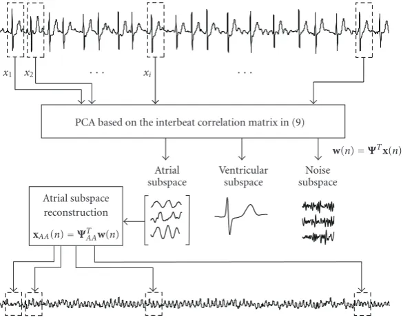
Atrial subspace reconstruction
xAA(n)=ΨTAAw(n)
Atrial subspace
Ventricular subspace
Noise subspace
w(n)=ΨTx(n)
PCA based on the interbeat correlation matrix in (9)
x1 x2 xi
Figure11: Block diagram of interbeat PCA to estimate the atrial activity during AF. The principal components are obtained by (10), and each of the signals in the different subspaces is given bywk(n). The reconstruction is made from the partitioned transformation matrix
Ψ=ΨV AΨAAΨN, generating the reconstructed atrial signalxAA(n) usingxAA(n)=ΨAAw(n) and concatenating back to recover the atrial
signal displayed at the bottom.
usually exhibits a recurrent pattern, although different QRST morphologies as well as minor variations in the QRST wave-form may occur. For the case when several consecutive beats from the same lead are extracted and PCA is applied to ex-ploit interbeat redundancy, the principal components, or-dered according to the eigenvalue sequence, are interpreted as follows.
(1) The most significant component is related to the main QRST waveform. In case of several QRST morpholo-gies, a principal component will represent each of the pat-terns.
(2) The next few components correspond to dynamics of the QRST waveform. In case of a very regular QRST mor-phology, these components may be missing.
(3) Subsequently, there are several components related to the atrial activity.
(4) The remaining components correspond to noise. In addition to the components, PCA outputs the projec-tion of each component has on each beat. Taking these con-siderations into account, the QRS complex and T wave can be removed at each beat by considering the projections of the ventricular components and removing them from the ECG signal. Equivalently, the same result would be obtained by es-timating the atrial activity at each beat from the projections of the nonventricular components (Figure 11).
Cancellation of ventricular activity using the single-lead approach is closely related to adaptive template subtraction, but with the advantage that dynamics in the QRST wave-form are also considered, thus producing a more accurate es-timate of the atrial signal. This technique has been applied to discriminate nonterminating from terminating AF episodes
from Holter recordings [65]. Spectral analysis of the esti-mated atrial signal revealed that terminating AF had a lower frequency (3.75–5.5 Hz) than nonterminating AF recordings (5.5–8 Hz) for the patients under study.
6.2. Multilead analysis
The atrial signal can be extracted by exploiting the spatial in-formation in multilead ECGs. By applying PCA to the 12-lead ECG, it is possible to remove redundant information contained in the different leads and synthesize them such that the principal components are uncorrelated. Hence, the most representative component is the one which corresponds to the ventricular activity since this activity exhibits the largest energy, whereas the next few components correspond to vari-ability in ventricular activity (cf. the single-lead case above). Among the next principal components, it is possible to find a signal which corresponds to the atrial activity.Figure 12
shows an example where PCA is applied to an AF episode, where the atrial activity can be identified as the fourth prin-cipal component, whereas the three first components contain ventricular activity. The detection of the atrial component can be performed using the FFT, since the extracted signal typically exhibits a dominant frequency peak between 3 and 12 Hz. The suitability of PCA for the extraction of the atrial signal has been proposed and validated in [63].
0 5 10
Time (s)
2 0 2 2 0 2 2 0 2 5 0 5 5 0 5 2 0 2 1 0 1 1 0 1
A
m
plitude
(mV
)
x8(n)
x7(n)
x6(n)
x5(n)
x4(n)
x3(n)
x2(n)
x1(n)
(a)
0 5 10
Time (s)
10 0 10 10 0 10 10 0 105 0 5 10 0 10 5 0 5 10 0 105 0 5
N
o
rm
aliz
ed
amplitude
w8(n)
w7(n)
w6(n)
w5(n)
w4(n)
w3(n)
w2(n)
w1(n)
(b)
Figure12: Example of atrial signal extraction during AF using a multilead PCA approach. (a) The original 8 ECG leads, wherex1 andx2are I and II limb leads, andx3tox8are the precordial leads, and (b) the corresponding principal components.
the observation of mixtures. Indeed, a BSS-based solution that not only exploits second-order statistics but also higher-order statistics to estimate the fibrillatory wave has been pro-posed [67].
So far, PCA has been applied to extract atrial signals for monitoring the effects of (1) antiarrhythmic drugs [63] and (2) linear atrial ablation [68]. After extraction of fibrillatory
waves, FFT has been applied to detect the main frequency, which was shown to decrease with the administration of ei-ther amiodarone (from 5.8 Hz to 4.9 Hz), flecainide (from 5.3 Hz to 4.7 Hz), or sotalol (from 5.9 Hz to 4.9 Hz) [63]. Similarly, fibrillatory frequency changes in response to lin-ear left atrial ablation have been monitored and the effect on fibrillatory frequency of roof and mitral isthmus lines have been quantified [68]. Fibrillatory frequency decreased from 5.66 Hz to 5.15 Hz with a greater decrease after left atrial roof ablation compared with mitral isthmus ablation (0.31 Hz versus 0.10 Hz). Even though there was a trend to lower baseline frequencies with successful ablation, this study was not powered to predict outcome, although an invasive study supports this conclusion [69].
7. BODY SURFACE POTENTIAL MAPPING
Body surface potential mapping (BSPM) refers to the record-ing and analysis of temporal and spatial distributions of ECG potentials acquired multiple sites on the torso. In contrast to the analysis of the 12-lead ECG, where wave amplitudes, intervals, and morphology are usually considered, BSPM is rather considered in terms such as the shape of the poten-tial distribution and the number and location of extrema. Since the electrodes that define such a map are closely spaced on the body surface, therefore containing considerable re-dundancy, PCA-based methods have been employed for data compression. It has been shown that spatial redundancy can be substantially reduced using the definition in (28) [70,71], thereby resulting in a subset of leads which contains much richer information than subsets of the original leads of the same size. From such a subset of leads, better separation can be made of different types of patients [72,73].
288 289 290 292 293 294 295 296 297 298 299 300 301 302 303 304 305 306 248 249 250 252 253 254 255 256 257 258 259 260 261 262 263 264 265 266 207 208 209 211 212 213 214 215 216 217 218 219 220 221 222 223 224 225 165 166 167 169 170 171 172 174 175 176 177 178 179 180 181 182 183 184 123 124 126 127 128 129 130 131 132 137 138 139 140 141 142
80 81 83 84 85 86 87 88 89 93 94 95 96 97
39 41 43 44 45 46 47 48 49 54 55 56
14 16 17 18
BSPM
Figure13: Data matrixDiwith one beat from a BSPM recording. The signal from leadlis plotted around the torso location where the
sensing electrode is located. The torso is displayed in an unfolded format, the right subplot corresponds to the back, the left one to the front, and the middle hole corresponds to the left axile.
QRS-KLT14
288 289 290 292 293 294 295 296 297 298 299 300 301 302 303 304 305 306 248 249 250 252 253 254 255 256 257 258 259 260 261 262 263 264 265 266 207 208 209 211 212 213 214 215 216 217 218 219 220 221 222 223 224 225 165 166 167 169 170 171 172 174 175 176 177 178 179 180 181 182 183 184 123 124 126 127 128 129 130 131 132 137 138 139 140 141 142
80 81 83 84 85 86 87 88 89 93 94 95 96 97
39 41 43 44 45 46 47 48 49 54 55 56
14 16 17 18
Figure14: Basis functionBn,lderived from the BSPM data displayed inFigure 13, using lead piling (Bn,lis obtained by depiling the
eigen-vector of order 14).
8. CONCLUSIONS
Several PCA-based strategies are available which exploit the fact that the ECG signal exhibits intrabeat, interbeat, and