Cue phrase selection methods for textual classification problems

(1)

Cue Phrase Selection Methods for

Textual Classification Problems

J.H. Stehouwer Master of Science Thesis Human Media Interaction

Research Group Human Media Interaction Faculty of Computer Science

University of Twente Enschede, The Netherlands

Graduation Committee: Dr. Ir. H.J.A. op den Akker

Dr. D.K.J. Heylen Ir. R.J. Rienks

(2)

(3)

Samenvatting

De classificatie van teksten en delen van teksten, maakt voor een belangrijk deel gebruik van het voorkomen van woorden en combinaties van woorden. Niet elk woord of woordcombinatie speelt een even duidelijke rol als indicator van de classificatie van een stuk tekst. Er is onderzoek gedaan naar methodes voor het selecteren van de meer indicatieve (opeenvolgende) woorden uit de verzameling van woorden en woordgroepen zoals deze in de teksten voorkomen. Deze, meer indicatieve, (combinaties van) woorden noemen we cue-phrases. Het doel van deze methodes is dan ook het eerst selecteren van de meest indicatieve cue-phrases. De geselecteerde verzameling woorden en groepen van woorden kan vervolgens worden gebruikt bij het trainen van het classificatiesysteem. Om deze methodes te bestuderen zijn een aantal experimenten uitgevoerd op een corpus van recepten uit een kookboek, en op een corpus van vergaderingen met vier deelnemers. Teneinde dit te bewerkstelligen is er ook een computer programma geschreven, hetgeen gebruikt is voor deze experimenten.

Voor de experimenten op het corpus van recepten is er gekeken of het mo-gelijk was de zinnen van recepten te classificeren in verschillende types. Denk hierbij aan een classificatie in types zoals onder andere “requirement” en “in-struction”. Voor de experimenten op het corpus van vergaderingen met vier deelnemers is gekeken of het, met enkel deze features, leerbaar is of een zin aan een individu of een groep gericht is. De persoon aan wie een uitspraak gericht wordt wordt ook wel de geadresseerde (Eng. addressee) genoemd.

De experimenten op de recepten leverden goede resultaten op, waarbij duidelijk wordt dat, een aantal van de in dit verslag besproken methodes geschikt zijn om woorden of woordcombinaties mee te selecteren. De experimenten op het vergaderingen corpus waren minder succesvol qua het volbrengen van de clas-sificatietaak. Wel zagen we vergelijkbare patronen qua de prestaties van de verschillende selectie methodes. Gezien de resultaten van Jovanovic kunnen we concluderen dat er voor deze classificatie meer nodig is dan enkel woorden.

(4)

(5)

Summary

The classification of texts and pieces of texts uses the occurrence of, combina-tions of, words as an important indicator. Not every word or each combination of words gives a clear indication of the classification of a piece of text. Research has been done on methods that select some words or combinations of words that are more indicative of the type of a piece of text. These words or combinations of words are selected from the words and word-groups as they occur in the texts. These more indicative words or combinations of words we call “cue-phrases”. The goal of these methods is to select the most indicative cue-phrases first. The collection of selected words and/or combinations thereof can then be used for training the classification system. To test these selection methods, a number of experiments has been done on a corpus containing cookbook recipes and on a corpus of four-participant meetings. To perform these experiments, a computer program was written.

On the recipe corpus we looked at classifying the sentences into different types. Some examples of these types include “requirement” and “instruction”. On the four-person meeting corpus we tried to learn, using only lexical features, whether a sentence is addressed to an individual or a group.

The experiments on the recipe corpus produced good results that showed that, a number of, the used cue-phrase selection methods are suitable for fea-ture selection. The experiments on the four-person meeting corpus where less successful in terms of performance off the classification task. We did see compa-rable patterns in selection methods, and considering the results of Jovanovic we can conclude that different features are needed for this particular classification task.

(6)

(7)

Preface

Science is what we understand well enough to explain to a computer. Art is everything else we do.

Donald Knuth

Five years ago I started studying Computer Science at the University of Twente. In these five years I learned a lot of things, not all of them directly related to Computer Science. As time went by the subject itself became more and more interesting, and I chose to specialise in Human Media Interaction, specifically the Machine Learning part thereof.

When I started on my final projects all kinds of ideas where up in the air, and I started by looking at the final thesis of van der Weijden and the thesis of Kats. Because of the work of van der Weijden I started looking at discussions in meetings, specifically at what discussions are.

The work of Kats and the work of Verbree turned me to the automatic selection of cue-phrases, a method suitable for text-classification problems where the problem can be solved using lexical features. To experiment with these cue-phrase selection methods a tool was made to run the experiments with.

One of the text classification problem I looked at is the recipe-classification task. Another classification task I learned of via Natasa Jovanovic and Rieks op den Akker. This task is concerned with the learn-ability of the addressee of sentences in meetings. Specifically to see if it was learnable whether an utterance is single or group addressed. A lot of time was spend on this problem.

I would like to thank several people for their contribution to this thesis. First of all I want to thank my parents and my little sister, who kept me motivated when things didn’t go as fast as I’d like. I want to thank my supervisors, especially Rieks, for the generous amount of usefull and timely feedback given during the whole process. And finally I wish to thank the Student Network Twente and Stichting Abunai for keeping me usefully distracted when I needed to get my mind of things.

All in all it has been a fun five years. In fact five years may be a little too fast to get out of here as there is so much left to learn.

(8)

(9)

CHAPTER

1

Introduction

It is not unusual these days to spend a lot of time in meetings. While these meetings themselves cost quite a bit of time, the time spend preparing for the meetings and time spend processing the results of the meeting is far greater. A significant amount of scientific work has been done on automating parts of these processes. The work presented in this thesis aims to aid this process, or at least provide some insights.

In the University of Twente itself, a good amount of recent research has fo-cussed on parts of the Augmented Multi-party Interaction project, or AMI for short. The AMI project aims to ‘augment’ meetings by giving all participants to a meeting valuable and important information about that meeting in a con-venient way. This information should help the comprehension of the meeting, streamlining it. This should be done automatically and without user interven-tion. The corpus of the AMI project consists of a set of role-played meeting augmented with some annotations, including (amongst others) dialogue acts, topic segmentation, gestures, gaze, addressee and dialogue act relations.

One of the topics that has been looked at recently is the visualisation of the structure of meetings, or more specifically the visualisation of discussions in meetings. For this van der Weijden designed a discussion annotation and visualisation method called Twente Argument Schema or TAS [vdW05, RR06b]. For a short description of TAS see appendix E. Some research has been done about the usability of TAS and the results presented in [RR06a] suggest that the application of TAS does help with the comprehension of the meeting structures. However, the definition of what a discussion actually is, is unclear. In chapter 2 we will look at this issue. We specifically look if there is agreement on the annotation from different annotators given our definition. Of these results a qualitative analysis is done using, amongst other things Adjacency Pairs and Dialogue Acts.

(12)

phrases. As Samuel, Carberry and Vijay-Shanker show in [SCVS99] cue-phrases are one of the most effective features when used for dialogue act tagging. It is likely that the methods presented in this paper generalise to other tasks than dialogue act tagging and to other corpora. Therefore we will discuss their cue-phrase selection methods in chapter 3 in detail.

Quite a bit of work has been done recently at the university that involves the automatic selection of cue-phrases to use as features while learning. Both Kats and Verbree used automatically selected cue-phrases in their research. The goal of cue-phrase selection methods is to select the most indicative (combinations of) words first. So a cue-phrase selection method is, for a certain classification task, better than another if the achieved accuracy rises faster in the beginning. It is also desirable to have computationally efficient cue-phrase selection methods.

In [Kat06] Kats used the cue-phrase selection methods from [SCVS99] on the IMIX sentence classification task. Verbree used a few of his own selection methods in [Ver06] on the TAS node sentence classification task. The methods used by both Kats and Verbree will be discussed in chapter 3. Using cue-phrase selection methods one can select appropriate “cues” and use those for learning. These cues are lexical cues, and therefore suitable for classification tasks where lexical features are adequate by themselves, or help the performance of the classification. In order to facilitate the experimentation with these different cue-phrase selection methods on different classification tasks and corpora a tool was written, in the chapter on cue-phrases this tool is also presented.

The first classification task on which the cue-phrase selection methods are tested is the recipe corpus. The recipe corpus, containing sentences from cook-book recipes, and the corresponding classification task are presented in chapter 4. The recipe classification task entails that each sentence is assigned a certain type, such as requirement, name, instruction blocking, etc.

The second task on which the cue-phrase selection methods are tested is that of the identification of the addressee of an utterance. Specifically to clas-sify whether an utterance is addressed to an individual or to a group. Addressing is an important part of communication [Gof81, NJN06] and helps disambiguate discussions in meetings. Jovanovic has produced excellent results in [NJN06] on identifying the addressee of an utterance. She finds out whom exactly the ut-terance is addressed to, a task more complex than our single or group addressed task. However for this she uses a number of computationally expensive features such as gaze and gesture information. The details of this task are explained in chapter 5. We only use the selected cue-phrases in most of the experiments, but also run a smaller series of experiments using dialogue acts and also the length of the utterance.

(13)

CHAPTER

2

Discussions

Previous work done by van der Weijden (in [vdW05]) produced a scheme for annotating discusions called TAS that aims to get a more detailed view of the “structure” of those discussions. TASs is discussed in detail in appendix E. TAS is applied to discussion segments, but how are those segments determined? Do human annotators agree on this? This chapter aims to look briefly at this issue and provide some footholds for future research. Discussions are an important part in meetings, as they are a means to settle differences in opinion.

An example of a discussion, as found in meeting IS1003c is given in figure 2.1. As can be seen participant C thinks it is an advantage of the intelligent controller that it can have voice recognition. Opposed to Participant C are in this, rather short, discussion participants A and D who think voice control would be a disadvantage.

This example conforms to the definition of discussion as found in [Rie06]:

“A dialogue,related to a single statement or proposition, on which not all participants agree.” (emphasis mine). What we want to know is: Is this definition complete enough for discussion annotation and what kind of features could be used to learn these annotations?. To see whether this definition alone is enough to provide a reliable annotation an annotation manual was created and discussions where annotated. The exact method used is explained in the next section.

C: Yeah , thats thats the advantage of intelligent controller . Even you h you have the controller S , I can [other] I can say channel three , so its c come to channel three , I dont have to [laugh] .[disfmarker]

D: No .

B: [laugh] Its [disfmarker] its [gap] [laugh] D: No , but this is disadvant disadvantage . A: Yeah , I think its a disadvantage . C: Its advantage .

(14)

2.1

Method

In order to answer the question we must first see whether different annotators can use this definition of discussions. In other words whether the annotators agree on the location of discussions as they are defined by this definition. It was decided that we would annotate discussions IS1003a, IS1003b, IS1003c and IS1003d from the AMI corpus. To do that an annotation manual was written. A tool called ArgumentA was used to annotate the discussions. ArgumentA was also used to mark discussions for TAS annotation and it was written by van der Weijden for his final project (see [vdW05]). The annotation manual that was written can be found in appendix B. With the results of this annotation we can then try to answer the questions.

The data collected consists of three annotators marking the location of all discussions in meetings IS1003a, IS1003b, IS1003c and IS1003d. The start and end points of all discussions where marked on the transcription, colouring the lines where the discussion-annotation denoted an end or a start of a discussion. These marked transcriptions are not included in this thesis because of large amount of pages they take up.

Due to the small amount of annotation data available, a quantitative analysis would not produce reliable results. So, a qualitative analysis, aided by a small collection of scripts, was performed.

The data that was available was used to extract some simple statistics. One of these produces for the start- and end-points of discusions several datapoints. These datapoint include the label the annotator marked the discussions with, the dialogue of the starting/ending utterance, the addressee of the dialogue act, the speaker of that dialogue act and the complete utterance that belongs to that dialogue act. This data is available in a tabular format in appendix C. In section 2.2 (below) we discuss the Dialogue Acts with which the AMI corpus is annotated.

To see whether there is a difference in the distribution of dialogue acts and addressing inside discussions compared to outside discussions information was compiled about this. Should these differences be large they could be exploited for use in automatic annotation of these discussions.

The number of dialogue acts inside and outside discussions where counted for each annotator for each discussion. These can be found in appendix 2.3. The distribution of Dialogue Acts inside and outside of discussions was also counted, these can be found in table 2.5. Finally words occurring inside and outside discussions in a meeting where counted for all three annotators for all meetings. The results of this will be discussed below, but the raw data will not be given as it would take up a lot of space. This was stored in one file per annotator, one file per discussion.

(15)

CHAPTER 2. DISCUSSIONS:2.2. Dialogue Acts

The results obtained in this way will be discussed below in section 2.3.

2.2

Dialogue Acts

As we look at the AMI dialogue acts at the start and end of discussions, as well as their distribution inside and outside discussions, they will be discussed here briefly. For a detailed description please see [AMI]. Dialogue Acts are a way of marking a transcription according to speaker intention.

An essential part of dialogue act coding is the determining where the bound-aries between the different DA’s lie. It is quite possible to have a DA span multiple utterances, for example “No, it’s not. It’s not.”. As well as that a single utterance may be split in multiple segments if necessary. For all the different DA-labels discussed below there are several examples as well as clear instructions to prevent common confusions in [AMI]. Now on to the DA’s:

Backchannel Short utterance in the background that doesn’t really stop the

current speaker. Typically used to communicate to the current speaker that the speaker of the backchannel is still listening.

Stall A short utterance, used when the speaker hasn’t figured out what to say, or to try to get or keep the attention of the group. Note thatStallitself isn’t really a dialogue act, just a convention used in the AMI project, since it is usefull to label every utterance, even those not really conveying intention (besides the ‘I want to keep speaking’ part).

Fragment A fragment is a segment that isn’t aStall, nor aBackchannelbut

doesn’t convey speaker intention.

Inform Gives information.

Elicit-Inform Requests information from someone else.

Suggest Suggests a course of action.

Offer The speaker expresses an intention of his/her own actions.

Elicit-Offer-Or-Suggestion The speaker wants somewhone to make a

sug-gestion or an offer.

Assess Expresses an evaluation (‘That would be good’, ‘yeah’, ‘it is a big num-ber’, etc.).

Comment-About-Understanding A DA for segments that indicate wether

the previous speaker was understood.

Elicit-Assessment A DA for segments that (tries to) elicit an assessment from a speaker.

Elicit-Comment-About-Understanding The speakers elicits a responce from

a (group of) speakers about wether the speaker was understood.

(16)

Be-Negative A social act that makes an individual or the group less happy.

Other Any segment that doesn’t fit with any of the above DA’s. For example

mumbling aloud, ‘Now, where was I?’.

AMI annotation also contains a relation annotation linking an utterance to another utterance. This is only done if the annotator thinks a relation exists. It only contains a few relations, namely:

Positive The target supports the intention of the source. For example (taken from [AMI]):

Positive Relation Example ...upon picking up a whiteboard pen and stepping up to the white-board for the first time...

C Okay | VERY NICE | alright

Negative The target rejects the source. For example (taken from [AMI]):

Negative Relation Example A Mm. So, some kind of idea uh with um um cel lular phone with

a a screen that wil l tel l you what, no . C NO, NO SCREENS | its too complex.

Partial The target partially supports but partially rejects the source. For

example (taken from [AMI]):

Partial Relation Example [C is drawing on the whiteboard]

D A kind of snake? A cobra?

C Yeah, uh | NOT REALLY, | a small cobra.

Uncertain The target expresses uncertainty about the source. For example

(taken from [AMI]):

Uncertain Relation Example C We can adapt only one switch, suppose here like we can make

two switches and if Im left-hander I use this switch to follow the main operations.

B I mean if its less than three uh then we can make it uh like a... D THREE BUTTONS, YOU MEAN?

2.3

Results

To evaluate, by hand, the degree of annotator agreement we look at the tran-scriptions marked with the start- and end-points of discussions. As stated before the discussions were annotated for all four meetings by three different annota-tors which we shall refer to as H (for Herman), J (for Jan) and R (for Rieks). Looking at the transcriptions it quickly becomes clear that annotators H and R seem to agree about the position on a decent amount of the discussions, though almost always with start and end utterances that lie a few utterances apart. In meeting IS1003d the disagreement between all annotators is quite large. It is quite likely that the reason why H and R agree some discussions is that, prior to the writing of the annotation manual, they discussed the nature of discussions in some detail, thus creating some sort of agreement. One example of such a discussion (from the IS1003b transcription) can be seen in table 2.1.

(17)

CHAPTER 2. DISCUSSIONS:2.3. Results

Sentence H J R

C: And just to have uh an idea , do you think you as the S

C: User Interface Designer to would it be possible to have less buttons and still have the same functionality and to have powerful remote control , you think it’s possible ? Sure ? Yeah ? D: Yeah .

D: Yeah , I think possible . Because we can [disfmarker] D: We can uh

D: mix uh several function in one button . C: Yeah .

D: So lets you [disfmarker] then you have less buttons . But I’m not sure [disfmarker]

C: Yeah , but do you think it will be easy to use ? Because if you have many functions just for S

one button it would be quite difficult for the user to know . A: Yeah , remember the user is not happy to read the C: Yeah , I think the [disfmarker]

B: The manuals . S

A: manual . It’s [disfmarker]

D: No you you can have a switch menu , so you can C: Yeah , but it has to be intuitive .

D: well for example [disfmarker]

D: Yeah , I think so . Like for for example you can uh you can category the function i i into several classes . Then

D: for um you can have a switch menu , so you put the switch menu to it it tend to this kind of this category of functions . Then you you put the switch button , then it

C: Yeah , okay . C: Okay , but [disfmarker]

D: switch to another category of functions . D: Yeah .

D: For example , if you have remote control you you can rem you can control your T V and also

you can control your uh recorder . B: With a [disfmarker]

D: So there’s a different functions , but i if you you [disfmarker] there’s a button you can switch

between control T V and control your recorder . E E

Table 2.1: An example of a discussion in which the Hand R agree on the discussions,

but have different starting points. Taken from the IS1003b meeting.

Sentence H J R

D: No y you do the minutes first , or ? S

A: What ? D: No ?

A: I I think I will let uh our User Interface Designer speak first , Mister David Jordan . D: Okay .

C: Yep . E

Table 2.2:An example of something of which annotator J believes that it is a

discus-sion, but H and R do not. Taken from IS1003c.

Very often it is seen that only annotator J thinks that there is a discussions, but that annotators H and R don’t agree with this. One such example (from discussion IS1003c) can be found in table 2.2.

J mostly sees discussions, when the others do not, when there is not a differ-ence of opinion, but a differdiffer-ence in beliefs of the participants. Such a differdiffer-ence of beliefs is often quickly resolved and mainly involves synchronizing informa-tion between the participants of the meeting. We, on the other hand, would like to have the differences of opinion annotated.

So we can state about these results that the overall inter-annotator agree-ment is poor. That, even though they agree on the nature of discussions, H and R still disagree most of the time about the exact start and end of discussions. H and R seem to agree about the position of most discussions, except in meeting IS1003d. This is also supported by the numbers shown in table 2.3 about the number of utterances inside and outside of discussions.

Appendix C contains tables listing, for the annotated beginnings and endings of discussions, the corresponding AMI Dialogue Act and information related to that Dialogue Act (the addressee, the speaker, the complete utterance belonging to that DA).

(18)

acts is quite different. For example the second discussion as annotated by J in IS1003a starts with a “Stall” Dialogue Act belonging to the utterance“So”, the corresponding TAS segment is “So the selling price of the product will be twenty five Euros . [laugh] Yeah . Yeah . [other] I S think its quite good price , yeah . And uh”. The start and end of discussions were annotated using the Argumenta tool, which used the TAS segmentation.

From the same data it also becomes clear that discussions tend to start on a Stall (35%), Suggest (11%), Asses (10%) , Inform (15%) , Elicit-asses (12%) or Elicit-inform (9%) while most discussions end with a Stall (13%), Backchannel (40%)), Comment-About-Understanding (5%), Asses (27%) and sometimes an Inform (10%). Related to this are the tables of the distribution of Dialogue Acts inside and outside discussions in the annotated meetings, these can be found in table 2.5. For example from the table for meeting IS1003c and annotator H, for which around 50% of the meeting is marked as discussion, we see for example a higher number of the “suggest” dialogue act ouside discussions. There are some differences between the dialogue act distributions inside and outside the annotated discussions for all annotators, with some DA’s being more common inside and others more common outside of discussions. While clear, these differences are not that large for the frequently occuring DA’s.

When looking at the numbers of words inside and outside of discussions no words which occur much more inside the discussions where found. Of the list of words, words that only occurred within discussions, or which occurred outside discussions infrequently, no words occurred frequently in the meeting. For example, though the wordswitch only seems to occur within discussions in meeting IS1003b it occurs only 6 times in the complete meeting. Most, around 95%, words that only occur within discussions, or only once or twice outside discussions occur in dicussions only 3 or fewer times. So no reliable indicators of discussions within the AMI meetings IS1003a/b/c/d where found.

Some data was also compiled which is only available for meetings IS1003b and IS1003d. The first set of this is the amount of group addressed utterances inside and outside of discussions, compared to the number of DA’s inside and outside discussions. This data can be found in table 2.4 compared to table 2.3. We can see in the data that the amount of group addressed DA’s is, proportionally, larger outside discussions (around 30%) than inside discussions (around 20%). However less than 30% of the total DA’s is group addressed, so the difference in the proportion of group-addressed DA’s can give no more than a possible indication of a discussion. The same, slight, differences are also in the second set of data, that of the speaker patterns of the annotated Adjacency Pairs, which can be found in Appendix D. However these differ a lot between IS1003b and IS1003d and between annotators also. Conclusions cannot be drawn.

2.4

Conclusion and Discussion

(19)

dif-CHAPTER 2. DISCUSSIONS:2.4. Conclusion and Discussion

H J R

IS1003a Inside 45 127 50

Outside 373 290 368

IS1003b Inside 169 357 269

Outside 524 336 424

IS1003c Inside 446 456 494

Outside 485 475 437

IS1003d Inside 885 1080 306

Outside 678 483 1257

Table 2.3: The number of dialogue acts contained in discussions and the number of

dialogue outside discussions for all annotated meetings.

H J R

IS1003b Inside 29 80 58

Outside 148 97 119

IS1003d Inside 247 308 81

Outside 247 114 341

Table 2.4: The number of group addressed dialogue acts contained in discussions and

(20)

(21)

CHAPTER 2. DISCUSSIONS:2.4. Conclusion and Discussion

ferent sorts. The discussions as annotated are continuous segments, it could also happen that a discussion is “split up” by some irrelevant material in between. It is undefined how the annotators should deal with this, but annotators can either annotate two separate discussions, or annotate it as one long discussion. A clear, and rather extreme, example of a difference of this sort occurs between annotators H and R in the first half of meeting IS1003d. For the one discussion annotated by R, H annotated six different discussions.

Annotators disagree on the exact start and end of discussions most of the time, though frequently, if they agree on the discussion in general, these differ only a few utterances. The difference between annotator J and annotators H and R seems to be primarily about the type of disagreement needed. To improve the definition it can be pointed out that the disagreement should present a difference of opinion, not a difference of beliefs. While a difference of beliefs is defined as a discussion by the used definition, it isn’t the type of disagreement that we would like to have annotated. A new, slightly improved definition could, for example, be: “A dialogue, related to a single statement or proposition, on which not all participants agree. The disagreement should be a difference of opinion, and not a difference in beliefs about the world.”. With this new definition, and a much improved annotation guide a new experiment should be performed as test. We unfortunately lack the time.

(22)

(23)

CHAPTER

3

Cue Phrases and MAW

Some combinations of words are indicative of the class of a piece of text given a classification problem, one combination more so than the other. These combi-nations cue us to a certain class, hence the name cue-phrases. There has been quite a bit of previous work done on cue-phrases, including the work of Kats and the work of Verbree, which is discussed in section 3.2, and the work of Samuel et al. ([SCVS99]) which was also used by Kats in [Kat06] and which is discussed in section 3.1. This work discusses cue-phrase selection methods. These methods have to goal of selecting the most indicative cue-phrases first.

As one will see there are different methods for cue-phrase selection. With this we mean a way to rank all possible cue-phrases in some order in such a way that the firstnselected cue-phrases will be more descriptive of one of the classes of the classification which one is trying to learn. This means that the performance gains observed, when one adds more cue-phrases as features, should be much larger for the first few cue-phrases than for the later cue-phrases. This desired behavior is clearly visible in figure 3.1. One cue-phrase selection method is better than another, for a certain task on a certain corpus, if it approaches the maximum accuracy the fastest. With the maximum accuracy being the largest accuracy obtainable using cue-phrases, to this value most selection methods converge.

We will first discuss the cue-phrase selection methods in some detail. Then we will conclude the need to build a computer program to perform experiments with these selection methods, and finally we will describe this tool.

3.1

Cue-Phrase Selection Methods

(24)

Figure 3.1: An example of the desired behavior of a cue-phrase selection method. In this case using the DCP method on the Recipe classification task with a J48 learner.

It is important to note that these methods for cue-phrase selection can be applied to any learning task where cue-phrases can potentially be used for clas-sification. This means that it is applicable to any task where lexical features can be used for learning. In [SCVS99] it is noted that the DCP (Deviation Conditional Probability) cue-prhase selection method outperforms the others. Which is rather unexpected since DCP is a new metric unlike Information Gain or Mutual Information. Samuel et al. used a Transformation Based Learner to achieve their results.

A few definitions which are used in the formulas below will now be listed.

p A possible cue-phrase.

d A target for a cue-phrase, Samuel et al. used cue-phrases for dialogue-act classification.

#(x) The frequency of an eventx.

P(x) The probability ofx.

P(x|y) The probability ofxgiveny.

D The number of different targets.

U The number of items in the training set, Samuel et al. used utterances.

p The set of utterances in whichpdoes not appear.

We will now discuss all the cue-phrase selection methods as they where used by Samuel et al. ([SCVS99]) and Kats ([Kat06]). In several places we will use the described method on an example possible cue-phrase. For this we will use the following example “corpus”:

Sentence Class

The house is on fire . A

The cat is not . B

What a day . B

(25)

CHAPTER 3. CUE PHRASES AND MAW:3.1. Cue-Phrase Selection Methods

COOC [SCVS99] discusses several cue-phrase selection methods, of these the

coocurrence metric is the simplest. Thecooccurrence metric simply

gives each possible cue-phrase a number equal to the highest cooccurrence it has with one of the targets. In [SCVS99] those targets are dialogue acts. The formula for COOC is as follows:

COOC(p) = max

d #(p&d)

When using our example corpus and the possible cue-phrase “The” the scores would be as follows. For the target “A” the cooccurrence score would be two, for the target “B” the score would be one, therefore the phrase gets a total score of two.

When using this method possible cue-phrases with a higher score are more likely to be cue-phrases. This means that the cue-phrase that co-occurs with one of the targets the most is the first to be selected. The COOC metric does not take into account the a-priory distribution of the targets it is suppsed to learn. For example if the word “the” occurs 100 times in utterances of type A, and less often in other types, the COOC score of “the” will be 100.

CP Another possible selection method is theconditional probabilitymetric. CP is a simple conditional probability of a cue-phrase given a target. The formula for CP is as follows:

CP(p) = max

d P(p|d)

When using our example corpus and the possible cue-phrase “the” the scores would be as follows. For the target “A” the CP score would be 1, for the target “B” the CP score would be 0.5, therefore the phrase gets a total score of 1.

When using this method possible cue-phrases with a higher score are more likely to be cue-phrases. Conditional Probability does take into acount the distribution of the targets, however it does not take into account the frequency of the dialogue acts directly. CP selects cue-phrases purely on the change of finding the cue-phrase in a sentence if that sentence is of the type target. For example if the cue-phrase “the” occurs in half the phrases of type A and less in other types, the CP score of “the” will be 0.5.

ENT The entropy metric tries to find a cue-phrases that correlate with a

single target frequently and infrequently with other targets. The entropy metric is based on the standard, and well-known, definition of entropy as it is covered in many sources such as on page 224 of [JM00]. This is covered by the entropy of the dialogue acts given a phrase:

EN T(p) =−X

d

P(d|p) log₂P(d|p)

(26)

1∗0, for the target “B” the partial score would be 0.5∗ −1, therefore the phrase gets a total score of−(0−0.5) = 0.5.

When using the ENT metric possible cue-phrases with a lower score are more likely to be cue-phrases. However a cue-phrase that occurs equally likely across all targets will get a good score when using this method. The method will then, incorrectly, flag this cue-phrase as containing usefull information. To eliminate this problem in [SCVS99] they examined differ-ent ways of accounting for the dialogue-act distribution. These differdiffer-ent metrics use the Kullback-Liebler distance, mutual information, the t-test and information gain.

S Theselectional preference strengthmetric is a special case of the Kullback-Leibler distance. It considers the difference between the distribution of targets given a possible cue-phrase and the a priory distribution of targets:

S(p) =X

d

P(d|p)[log₂P(d|p)−log₂P(d)]

When using our example corpus and the possible cue-phrase “the” the scores would be as follows. For the target “A” the partial score would be 1∗(0 + 1), for the target “B” the partial score would be 0.5∗(−1 + 1), therefore the phrase gets a total score of 1.

When using the S metric possible cue-phrases with a higher score are more likely to be cue-phrases. This metric is discussed for instance on MathWorld1_{. It measures the difference between two discrete distributions}

and gives this distance a number. Note however that it is not a true distance measurement since, as can be seen clearly from the formula and what is also noted on mathword, the distance between p and d is not equal to the distance between d and p.

MI Themutual informationmetric measures the reduction of uncertainty to

an utterance’s target when the utterance contains the possible cue-phrase:

M I(p) =P(p)X

d

P(d|p)[log₂P(d|p)−log₂P(d)]

When using our example corpus and the possible cue-phrase “the” the scores would be as follows. For the target “A” the partial score would be 1∗(0 + 1), for the target “B” the partial score would be 0.5∗(−1 + 1), therefore the phrase gets a total score of 3₄∗1 = 3₄.

When using the MI metric possible cue-phrases with a higher score are more likely to be cue-phrases. The Mutual Information metric as given in [SCVS99] closely resembles the selectional preference strength metric. All remarks for that metric are also valid here.

TTEST The t test metric measures the statistical difference between two

distributions. In this case the difference between the a priori distribution of targets and the distribution of targets given a possible cue-phrase.

(27)

CHAPTER 3. CUE PHRASES AND MAW:3.1. Cue-Phrase Selection Methods

T T EST(p) = #(p) s

X

d

D2₋_D

[D#(p&d)−#(p)]2_{+ [}_D_#(_d₎₋_U_]2

When using the TTEST metric possible cue-phrases with a higher score are more likely to be cue-phrases.

IG The information gain metric measures the reduction in entropy of the

targets resulting from partitioning utterances based on the possible cue-phrase:

IG(p) =X

d

[P(p)P(d&p) log₂P(d&p)+P(p)P(d&p) log₂P(d&p)−P(d) log₂P(d)]

When using the IG metric possible cue-phrases with a higher score are more likely to be cue-phrases. Information Gain is a frequently used metric within machine learning, for instance in the weka toolkit ([IHW05]) it is used in various learning algorithms such as the J48 and ID3 tree-based classifiers.

D Thedeviationmetric is the first of the two new metric proposed in [SCVS99]. As elaborated in [SCVS99] there are two ways in which a cue-phrase may fail; First of all it may beunsound, meaning that the left-to-right rule, IF cue-phrase THEN target, applies incorrectly in some cases. Sec-ondly a cue-phrase may be incomplete, meaning that it does not occur in all utterances of the type it is a cue-phrase for. In [SCVS99] a single penalty point is assigned for each unsound and incomplete instance.

Thedeviationmetric adds the unsoundness and incompleteness of a

pos-sible cue-phrase together. This means that the D method is a measure of the number of times miss-classification would occur when using the cue-phrase as a completely reliable indicator of a class. It counts the number of times the cue-phrase

D(p) = min

d∗ [#(p&d

∗_{) +} X

d6=d∗

#(p&d)]

When using our example corpus and the possible cue-phrase “the” the scores would be as follows. For the target “A” the partial score would be 0 + 1, for the target “B” the patrial score would be 1 + 2, therefore the phrase gets a total score of 1.

The score for the best target for this possible cue-phrase is selected. When using the D metric possible cue-phrases with a higher score are more likely to be cue-phrases.

DCP Because, like COOC, the D metric does not take into account the a priori distribution of targets another metric was introduced: deviation

condi-tional probability. The deviation conditional probability method

(28)

AUTOMATICALLY SELECTING USEFUL PHRASES FOR DIALOGUE ACT TAGGING9

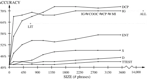
IG COOC CP MI 70% 40% 46% 52% 58% 64% ACCURACY 0

SIZE (# phrases)

3600 14,000

450 900 1350 1800 2250 2700 3150

LIT ALL ENT IG TTEST DCP D S

Figure 5. Size versus accuracy without the filter

5.1. The CutoffPoints

Since the methods are supposed to rank dialogue act cues higher than other phrases, we should be able to separate the dialogue act cues from the other phrases. To test this, we applied various cutoffpoints to each method to determine how many lower-ranking phrases may be removed before accuracy begins to decrease. We wanted to investigate the cutoff

points in isolation, so the lexical filter was not used in this set of experiments. Figure 5 presents the accuracy of each method as a function of the number of phrases used. The ALL and LIT sets are also included in the figure, for comparison. (For clarity, COOC, CP, and MI are not shown in the figure, because their curves are similar to IG’s curve.)

Four methods, TTEST, D, S, and ENT, produced accuracies significantly11_{below LIT}

when 25% (3558) of the 14,231 phrases were selected. This implies that many dialogue act cues were ranked in the bottom 75% by these methods, suggesting that there may be a problem with these phrase orderings. On the other hand, for four methods, IG, COOC, CP, and MI, we could remove more than 13,000 phrases without significantly affecting the accuracy. These methods also produced significantly higher accuracy scores than the LIT set. Therefore, automatic methods can select phrases that are better for dialogue act tagging than the cue phrases found in the literature.

However, DCP was the only method that produced a significantrisein accuracy over ALL. With cutoffpoints from 10% (1423) to 25% (3558), DCP’s accuracy was significantly

11

In all of the experiments in this paper, the differences were analyzed for statistical significance with the t test (Levine 1981) or the Tukey “honest significant differences” test, which is an extension of the t test that is appropriate for comparing more than two distributions. (Masterson 1997)

Figure 3.2: The results for all cue-phrase selection methods from [SCVS99], image

from [SCVS99].

of the chance of miss-classification when using the cue-phrase as a com-pletely reliable indicator of a class. It sums the chance the cue-phrase doesn’t occur in a sentence of the correct class and summed with the total chance the cue-phrase occurs in other classes.

DCP(p) = min

d∗ [P(p|d

∗_{) +} X

d6=d∗

P(p|d)]

When using our example corpus and the possible cue-phrase “the” the scores would be as follows. For the target “A” the partial score would be 0 + 0.5, for the target “B” the patrial score would be 0.5 + 1, therefore the phrase gets a total score of 0.5.

When using the DCP metric possible cue-phrases with a lower score are more likely to be cue-phrases ([SCVS99]). In [SCVS99] this is best per-forming cue-phrase selection metric.

When testing these cue-phrase selecting methods Samuel, Carberry and Vijay-Shanker found that the DCP method worked best, followed by IG, COOC, CP and MI. The other methods performed poorly. Their results are summed up in figure 3.2. They also used a lexical filter, which is described as:

IF a phrase p has a subsequence p that is ranked higher AND both p and p were selected for the same target THEN remove p

When using this form of lexical filtering they found that filtered-DCP performed no better then regular DCP. However, filtering it converged on the best result faster (while increasing the number of used cue-phrases). They found that the other methods performed slightly better filtered that non-filered. The results for DCP and IG are shown in figure 3.3.

(29)

CHAPTER 3. CUE PHRASES AND MAW:3.2. The work of Kats and the work of Verbree

12 PACLING’99, Waterloo, Canada

with the lexical filter without the lexical filter 70%

ACCURACY

0

SIZE (# phrases)

300 600 900 1200 1500 1800 2100

55% 58% 61% 64% 67% DCP IG

Figure 8. Size and modified filter versus accuracy

6. DISCUSSION

This paper presented an investigation of various methods for selecting useful phrases. We argued that the traditional method of selecting phrases, in which a human researcher analyzes discourse and chooses general cue phrases by intuition, could miss useful phrases. To address

this problem, we introducedautomaticmethods that use a tagged training corpus to select

phrases, and our experimental results demonstrated that these methods can outperform the manual approach. Another advantage of automatic methods is that they can be easily transferred to another tagged corpus.

Our experiments also showed that the effectiveness of different methods on the dialogue act tagging task varied significantly, when using relatively small sets of phrases. The method that used our new metric, DCP, produced significantly higher accuracy scores than any of the baselines or traditional metrics that we analyzed. In addition, we hypothesized that repetitive phrases should be eliminated in order to produce a more concise set of phrases. Our experimental results showed that our modified lexical filter can eliminate many redundant phrases without compromising accuracy, enabling the system to label dialogue acts effectively using only 5% of the phrases.

There are a number of research areas that we would like to investigate in the future, including the following: We intend to experiment with different weightings of unsoundness and incompleteness in the DCP metric; we believe that the simple lexical filter presented in this paper can be enhanced to improve it; we would like to study the merits of enforcing frequency thresholds for methods that have a frequency bias; for the semantic-clustering technique, we selected the clusters of words by hand, but it would be interesting to see

Figure 3.3: The results for the cue-phrase selection methods DCP and IG from

[SCVS99] when used with lexical filtering, image from [SCVS99].

3.2

The work of Kats and the work of Verbree

Kats

Amongst other features Kats uses automatically selected cue-phrases to deter-mine sentence types for a Question Answer system, constructed as part of the IMIX research program. For this Kats used the cue-phrase selection methods as proposed by Samuel et al. ([SCVS99]), with a few differences. First of all he used regular expressions as cue-phrases instead of n-grams, secondly he used a list of ncue-phrases, one list for each classification target, as a single feature instead of having each cue-phrase as a separate feature. He concludes that the COOC, DCP and IG metrics performed the best if used in this way with lexical filtering turned on.

As we use the cue-phrase selection methods proposed by Samuel et al. our-selves they are discussed below in section 3.1.

Verbree

In his thesis [Ver06] Verbree uses several cue-phrase selection methods to aid in the classification of sentences into TAS node types, TAS is discussed in appendix E. Though he selectednuni-grams,nbi-grams,ntri-grams andnquadri-grams that is irrelevant for the ranking method employed.

Select1/3Normalizedis what Verbree calls the first cue-phrase selection

method he uses. The S1/3N method selects ngrams only if it matches two conditions. First it must occur at least 3 times in the training set, secondly after normalisation it must have an occurrence ratio which is equal or bigger than 1

3. With an occurance ratio Verbree means that in more than 1 3 of the

cases it appears in sentences of a certain typeif all sentence types would occur as frequently as the others.

The second cue-phrase selection method used by Verbree he callsDROPn. In this method a cue-phrase is selected if it matches two conditions. First it must occur at least 3 times in the training set. Secondly there must be n sentence types in which the cue-phrase does not occur. In [Ver06] Verbree used DROPn

(30)

The third and final cue-phrase selection method used by Verbree he calls TOPx. TOPx ranks the cue-phrases and then selects the top xof them. By selecting only the most predictive cue-phrases a lot of “noisy” cue-phrases are eliminated. The ranking score is based on two assumptions. Firstly Verbree assumes that“Of two ngrams, the ngram which is more biased (after normal-ization) to a specific type (. . . ) has a bigger probability of being the cue-phrase than the other.”. Secondly he assumes that cue-phrases which occur more often, if they are equaly biased, are better. His ranking formula is the product of the number of times the cue-phrase occurs in sentences of type X and the part of the ‘ngram-space’ occupied by nodes of type X.

Conceptually, based on the two assumptions, this resembles CP, with the small difference that CP doesn’t take the number of times a cue-phrase occurs into account. However, in practise it is a multiplication of the CP and COOC methods together. Unfortunately the number of times a cue-phrase occurs has a much bigger influence on the final number than the occupation of the “ngram-space”. After all the the occurrence number can be infinitely large, while the part of the space cue-phrase occurs in is expressed as a fraction ([0,1]). All in all TOPxremains very biased to often occurring n-grams, selecting those as cue-phrases, for example the word “the” occurs very often in English texts.

Verbree notes that he achieves slightly better results when selecting cue-phrases based on their order. Meaning selecting n cue-phrase uni-grams, n

bi-grams, n tri-grams and n quadri-grams. However the order-specific cue-phrase selection method he employs selects more n-grams if the selection is done order-specific. Then again, as shown in [SCVS99] higher-order n-grams can add something even if lower-order n-grams with the same words are already selected, unless those are selected for the same class.

Another technique Verbree explores is that of compression. This means that all cue-phrases indicating a certain class are grouped together as a single feature. For each utterance this feature has as value the number of times a cue-phrase from its list occurs in that utterance. We do not use compression in our experiments as it performs worse than individual cue-phrases.

3.3

Building MAW

When we look at the list of different cue-phrase selection methods we see that, in order to perform a meaningful number of experiments, and to allow others to also perform comparable experiments, we needed a tool. After some investigation it was decided that it was easier to write such a tool from scratch than to adapt the code used by Verbree for his experiments for [Ver06]. The tool reads in a corpus, uses that data to create a training and a testing-set and extracts features from each sentence/utterance/block (corpus dependent). For the learning part the tool hooks into the well-known WEKA toolkit and uses the classifiers found therein. For more information on the WEKA toolkit see [IHW05]. The name

“MAW” was chosen for this project, the name stands forMAW And WEKA.

(31)

CHAPTER 3. CUE PHRASES AND MAW:3.3. Building MAW

plotted. In order to determine how to produce the desired tool a commented concept configuration file was written;

//general note: comma seperation for multiple items. [general]

corpus=...

corpustype=... // Should be a valid project.maw.readers.CorpusReader

corpusargs=... // Arguments for the Corpus (basicly: what features to read in) (:seperated) outfile=... // Outputs the results and confusion matrixes here

plot=... // Yes or No NOTE: if plot=yes then all plotoptions are mandatory! plus linelables and restvals // must have the same numberof different items as toplot

plottoplot=trainingsize:1,2,3,4;F0,F1,F2,F3:1,2,3,4 // the thing to plot and all its values, seperated by // ; for multiple lines

plotrestvals=F0,F1,F2:1|F3:2;trainingsize:1 // the values of the other things that ARE ITERATED OVER // ; for multiple lines

plottitle=... // title of the plot

plotlinelabels=line1;line2 // labels of the lines plotxlbl=... // X-axis label

plotylbl=... // Y-axis label plotfile=... // Save the plot somewhere

confidence=0.95 // the desired confidence interval for the delta values

usesparseinstances= // Yes or No, wether to use sparseinstances, only usefull if you think it might be ;P // (read api on weka.core.SparseInstance and use common sense) For a small number of features "no" is recommended [features]

F0=... // A valid project.maw.features.Feature

F0_args=.... // arguments (for example what feature to train on) F0_name=.... // the "name" of the feature

F1=... F1_args=... F1_name=... [training]

testsize=... (the number of corpusitems to use for training) tolearn=F1 // which feature to learn

learner=...//which weka classifier to use

learnerargs=...//arguments for the classifier SPACE SEPERATED !(different then elsewhere) [iteration]

iterations=10//number of normal iterations

trainsizes=...,...,...//comma seperated list of training-sizes (in CorpusItem’s) F0=...,...,... //multiple iter arguments for F0

F2,F3,F4=...,...,... //iterate over arguments and give the current one to F2, F3 and F4.

Note that the use of the word “feature” in the configuration file can point to several things. There are corpusfeatures i.e. raw features already encoded directly in the corpus such as the text of an utterance and annotations, there are feature classes i.e. features implementing project.maw.features.Feature that generate proper features, and finally there are proper features i.e. features as they are actually used in learning.

From this concept configuration file it was determined that the feature-generators, the corpus-type, the used classifier and the iteration had to be easily changeable. A basic package structure was created with interfaces for the creation of feature generators and corpus readers. It must be noted that the feature generators must ‘fit’ the data as read in by the corpusreader. The basic structure of the final program can be seen in figure 3.4.

After the creation of the basic framework two corpusreaders and several feature generators where created. As far as the corpus readers are concerned, one was build to read in the recipe corpus and one to read in the AMI corpus. For the features first a generic nominal feature was created and a “number of words” feature. The generic nominal feature just repeats the contents of a specific corpus feature, for example what the dialogue act of an utterance is. The “number of words” feature simply counts the number of words in an corpus feature (words are sequences of one or more characters seperated by a space).

(32)

maw

writers readers features data corpus

Stats Plotter

MAW GenIter Results Writer

ConfigFile Reader Corpus

Reader Feature

Results Arguments

Corpus Item Corpus

Figure 3.4: The structure of the maw program, only lists the most important classes

(33)

CHAPTER 3. CUE PHRASES AND MAW:3.3. Building MAW

feature generator. This set of cue-phrase selection feature generators support the selecting ofxn-gram cue-phrases each iteration, meaning that each iteration can have a different number of features generated where each generated feature is the number of times the selected cue-phrase at that position occurs in the utterance.

(34)

(35)

CHAPTER

4

Recipes

4.1

The Recipe Corpus

In [TA06] Alofs and Latour attempted to create an automated sentence classifier for QA systems. This classifier would work in the recipe, as in recipes for cooking, domain and classify the sentences in different types. For this they used a number of features and a loglinear maximum entropy classifier. In [Rat97] Maximum Entropy models are explained clearly and in detail.

Alofs and Latour didn’t yet have a corpus for this domain. They developed a system of sentence classification specific to the recipe domain and annotated the corpus with these sentence types. They hand-annotated all 3100 sentences of the recipes. Using their annotation guide and sentence classification they managed to achieve a Cohen’s Kappa of 0.88 on this task. This means that they achieved a very high inter-annotator agreement on this task.

The final categories on which Alofs and Latour decided are as follows:

Requirement A requirement is something needed for cooking the dish such

as an ingredient or a utensil used for preparing the dish. They note that these are usually listed at the beginning of a recipe or separate from the bulk of the recipe text.

Instruction Blocking “An instruction is a description of an action required

to prepare the dish.” An instruction blocking is an instruction where, during the time that the described task takes, the attention of the cook is required. This includes for instance chopping up vegetables or whipping cream.

Instruction Non-Blocking An instruction non-blocking is an instruction where,

during the time that the described task takes, the attention of the cook is only required sporadically. For example “bring the water to a boil”.

(36)

Category # of sentences mean length 95% confidence δ

name 136 3.04 0.374

ins-block 903 11.21 0.361

suggestion 73 9.01 1.021

ins-nonblock 426 12.45 0.545

emphasis 30 9.57 1.946

requirement 1072 4.08 0.217

inf-irrelevant 38 6.76 1.847

signal 296 1.22 0.083

inf-relevant 80 4.84 0.517

explanation 13 12.77 4.129

other 33 8 2.441

Table 4.1: A few simple statistics on the recipe corpus. This table contains per

sentence category the number of sentences in that category, the avarage sentence length

and the 95% confidence intervalδ(delta).

to help spot problem or determine the time a step in the cooking process takes. For example “the pizza is done when the cheese has melted”.

Suggestion According to Alofs and Latour a suggestion is a sentence that

describes an action that could add a twist to the disc or that could change the dish more to the cooks liking. For example “this dish goes well with a fresh salad”.

Explanation Alofs and Latour specify that an explanation“explains the

rea-sonign behind an instruction, suggestion, requirement or emphasis”. For example “this prevents the dish from getting burned.”.

Information Relevant to Cooking The information relevant to cooking class

contains the sentences in the recipe that contain information relevant to the cooking process such as preparation time, number of plates and nutri-tional information. For example “283 Kcal per person”.

Name The name of the dish.

Information Irrelevant to Cooking Information about the recipe that isn’t

relevant to cooking. For instance the name of the author, origin of the dish and a description of the dish. For example “this recipe is typical for the south-taiwanese kitchen”.

Signal Signals indicate the structure of the recipe. For example “ingredients”, “preparation” and the like.

Other The other class is the bucket class, it contains everything that does not fit in any of the other categories. For example “Bon appetite”.

(37)

CHAPTER 4. RECIPES:4.2. The Recipe Task, and Experiments

4.2

The Recipe Task, and Experiments

For the learning task Alofs and Latour used a mix of features. They used the complete sentence as a feature. They used a list of all unigrams, bigrams and trigrams of tokens in a sentence as feature. Also the number of words in a sentence was used because they reason it should be a good indication of certain classes such as requirement, name, signal and inf-relevant. These types of sentences are typically smaller than other sentences. They also included unigrams, bigrams and trigrams of Part-Of-Speech tags. For this they used the Medium-sized CGN tagset as they had access to a tagger that tags Dutch sentences with these tags. For more information on the CGN tagset see [vE04]. Using this combinations of these features they managed to score results of 88.2% when using the wordcount, word unigrams, bigrams and trigrams and Part-of-Speech tag unigrams. When just using the words features they managed to get results of up to 83.7%. When merging the blocking and non-blocking instruction classes the performance of the classifier could be boosted up to 93%. s Using the recipe classification task as outlined above a series of experiments where performed. For these experiments we wanted to look at the suitability of using automatically selected cue-phrases as features for the classifier. As Alofs and Latour where quite successfull in [TA06] when using all possible cue-phrases, up to length 3, as features for the Maximum Entropy learner this task should be very well suited to cue-phrase selection. We should see large gains in the first few hundred selected cue-phrases and smaller gains later on, indicating that the most indicative phrases have been selected first. In order to test this the experiments as described in [SCVS99] where recreated, only this time for the recipe corpus and the recipe sentence classification task. We can then compare the results obtained with the results of Alofs and Latour and also with the results that will be achieved on the addressee identification task (discussed in chapter 5. The experiments that we performed where:

1. For all of the automatic cue-phrase selection methods as outlined in chap-ter 3 we ran the following experiment. We selected different amounts of cue-phrases, specifically 0, 200, 400, 600, 800, 1000, 1200, 1400, 2000, 1600 and 3200 cue-phrases. These selected cue-phrases where then used as features on all sentences in the training set. For these experiments the J48 classifier as supplied in the WEKA toolkit was used. Verbree, in [Ver06], found this learner very effective. The experiments where run multiple times.

This set of experiments was run to look at the performance of the different cue-phrase selection methods compared to each-other and to see if the recipe classification task is learnable using cue-phrase selection.

(38)

This second set of experiments was run to look at the effect of lexical filtering, compared to the first set of experiments.

3. Later on we also ran an experiment, using the DCP cue-phrase selection method and the J48 learner. For the number of cue-phrases we again used 0, 200, 400, 600, 800, 1000, 1200, 1400, 2000, 1600 and 3200 cue-phrases. This time we added one extra feature, namely the number of words in a sentence. For this feature a word is defined as a sequence of one or more characters separated by whitespace. The experiments where run multiple times.

This experiment was run to see if the addition of the number of words would have an impact.

4. A final, small, experiment was run that tested the usefulness of the Na¨ıve-Bayes classifier from the WEKA toolkit. DCP was again used as the cue-phrase selection method. Once again 0, 200, 400, 600, 800, 1000, 1200, 1400, 2000, 1600 and 3200 cue-phrases where selected. This time also with the number of words of the sentence as feature. This experiment was also run multiple times.

This final set of experiments was run to see if the usage of another classifier, in this case Na¨ıveBayes (as also used by Jovanovic in [NJN06]), has an impact on performance.

With this small series of experiments we hope to show that the cue-phrase selection methods as proposed in [SCVS99] generate a suitable set of features for a generic classification task (where one can suffice with lexical features). The final two experiments have as purpose to evaluate the suitability of the Na¨ıve-Bayes classifier, as this was used extensively by Jovanic in [NJN06] (more on this in chapter 5). The results of these experiments are presented and discussed below.

4.3

Results

In this section the results for the recipe task experiments will be discussed. Each experiment, as outlined above, will be discussed separately.

As these are two terms we use in this discussion we will now define Precision and Recall. Precision and recall are two, commonly used, measurements of performance. The used definition of precision is, for classification T, the number of sentences correctly tagged with T divided by the total numver of sentences tagged with T. This is expressed in the following formula:

precision(T) =# correct with T # tagged with T

The used definition of recall is, for classification T, the number of sentences correctly tagged with T divided by the number of sentences that should be tagged with T. This is expressed in the following formula:

recall(T) = # correct with T

(39)

CHAPTER 4. RECIPES:4.3. Results

[general]

corpus=/Users/qadn/Desktop/Master_thesis/Recepten-Corpus.txt corpustype=project.maw.readers.RecipeCorpusReader corpusargs=type:sent:pos

outfile=/Users/qadn/Desktop/recipe-TTEST.txt plot=yes

confidence=0.95 confusionmatrix=yes

plottoplot=F0:0,200,400,600,800,1000,1200,1400,2000,2600,3200 plotrestvals=trainingsize:2500

plottitle=TTEST plotlinelabels=TTEST plotxlbl=Number of Phrases plotylbl=Accuracy

plotfile=/Users/qadn/Desktop/recipe-TTEST.eps usesparceinstances=yes

[features]

F0=project.maw.features.PhraseTTESTFeature F0_args=sent:type:3:yes

F0_name=ENT

F1=project.maw.features.GenericNominalFeature F1_args=type

F1_name=type [training] testsize=600 tolearn=F1

learner=weka.classifiers.trees.J48 learnerargs=

[iteration] iterations=10 trainsizes=2500

F0=0,200,400,600,800,1000,1200,1400,2000,2600,3200

Figure 4.1: An example configuration file for the recipe classification task. This

particular configuration file constructs an experiment using the TTEST cue-phrase selection method for selecting the cue-phrases with a trainingsize of 2500 sentences and a testingsize of 600 sentences. Lexical filtering is used.

In short, precision is a measure of the accuracy of a classification, and recall is a measure of the completeness of a classification. If a certain class has a high precision rating, but a low recall then too few utterances are labeled with it. On the other hand, a low precision and high recall means that too many utterances are labeled with it.

1. The first set of experiments as run on the recipe classification task uses all different cue-phrase selection methods, as introduced in [SCVS99] and discussed in chapter 3, on the recipe corpus. With each of these methods 0, 200, 400, 600, 800, 1000, 1200, 1400, 2000, 2600 and 3200 cue-phrases where selected to be used as features. The learning was done using the J48 classifier from the weka toolkit using MAW. The results of these ex-periments can be found in table 4.2.

Most cue-phrase selection methods get good results already when selecting only 200 cue-phrases, DCP lags a bit behind with good results from 400 cue-phrases. In [SCVS99] DCP was also observed to lag behind in the beginning. The exception to this are the ENT, S and TTEST methods. These also performed quite badly in [SCVS99]. The performance achieved, as seen from the results, varies 76% and 82%. It is noticeable that the achieved performance of the classification seems to sometimes peak early and then go down slightly again, such as in the results of, amongst others, COOC. It should be noted however that the results reported in [SCVS99] show the same small valleys.

Strangely enough the D (ordeviation) cue-phrase selection method seems to perform quite well. In [SCVS99] this was one of the worst performers.

(40)

reported in [TA06]. Their results, without adding Part-of-Speech n-grams as features1, are slightly better.

We see that the COOC,CP,D, DCP, IG and MI methods show the desired behavior: fast increase for a small number of cue-phrases, with the increase tapering of for larger number of cue-phrases.

2. For the second set of experiments we performed the same experiment as above, but with a small difference. This time the lexical filtering, as proposed in [SCVS99], was used. As explained before in chapter 3 the lexical filtering removes possible cue-phrases of which a sub-ngram has already been selected for the same target. The results of this set of experiments can be found in table 4.3.

Most phrase selection methods get good results at 200 selected cue-phrases. again with DCP lagging. Just like the previous experiment we see the TTEST, S and ENT methods not performing as well as the rest. Once again we observe the small valleys in the results.

When comparing these results with the results of the previous experiment (as they are listed in table 4.2) we notice that overall the performance is better with most of the methods (except TTEST, S and ENT) achieving an 80% or better accuracy. Especially the COOC, CP and IG methods benefit from the lexical filtering. However the results of the MI cue-phrase selec-tion method are worse with filtering than without filtering, in [SCVS99] lexical filtering improved its results.

Overall the results achieved in these experiments are in line with those reported in [TA06]. Their results, without adding Part-of-Speech n-grams as features, are slightly better.

3. For the third set of experiments on the Recipe corpus we used the DCP cue-phrase selection method to select 0, 200, 400, 600, 800, 1000, 1200, 1400, 2000, 2600 and 3200 cue-phrases. The J48 learner was used again and the experiment was run several times. This small set of experiments will be reported in a bit more detail.

A plot of the results can be found in figure 4.2, with a corresponding confusion matrix of one of the runs in table 4.4. This confusion matrix was taken from a single run in which 3200 cue-phrases where selected as features. Of the same run an recall-precision table is included as well in table 4.5.

From the plot we can see that using the DCP selection method shows the desired behavior, with the first n cue-phrases delivering the biggest increase in accuracy.

The same set of experiments was run, but this time with the addition of the number of words in a sentence as feature. The results of these can be found in figure 4.3 for a plot of the results, in table 4.6 for the confusionmatrix of a single run when selecting 3200 cue-phrases and in table 4.7 for the recall and precision table of that same run.

1_{They also produced even better results when using part-of-speech n-grams, however we do}

(41)

CHAPTER 4. RECIPES:4.3. Results

Looking at the results we see that the addition of the number of words

Cue phrase selection methods for textual classification problems

Cue Phrase Selection Methods for

Summary

Contents

CHAPTER

CHAPTER

Method

Dialogue Acts

Results

Conclusion and Discussion

CHAPTER

Cue-Phrase Selection Methods

AUTOMATICALLY SELECTING USEFUL PHRASES FOR DIALOGUE ACT TAGGING9

ACCURACY

The work of Kats and the work of Verbree

Building MAW

CHAPTER

The Recipe Task, and Experiments

Results