Practical Radio Link Resource Allocation for Fair QoS-Provision on OFDMA Downlink with Partial Channel-State Information

Volume 2009, Article ID 602856,16pages doi:10.1155/2009/602856

Research Article

Practical Radio Link Resource Allocation for Fair QoS-Provision

on OFDMA Downlink with Partial Channel-State Information

Ayman Alsawah and Inbar Fijalkow

ETIS, CNRS, ENSEA, University Cergy-Pontoise, 6 Avenue du Ponceau, 95000 Cergy-Pontoise, France

Correspondence should be addressed to Ayman Alsawah,[email protected]

Received 13 February 2008; Revised 6 June 2008; Accepted 22 July 2008

Recommended by Shinsuke Hara

We address the problem of resource allocation on the downlink of an OFDMA single-cell system under fairness constraints with limited channel state information (CSI). Target QoS corresponds to a minimum user data rate, a target bit-error rate and a maximum BER-outage probability. The channel model includes path-loss, shadowing, and fading. The only available CSI is the channel average gain of each user. This partial CSI defines ashadowed path-lossthat yields a modified user distribution. Resource allocation is based on theshadowed user distributionthat we characterize analytically. Thus, under the target QoS, we provide the optimal resource allocation that maximizes the user rate. Compared to full-CSI-based allocation schemes, our solution offers a significant complexity and feedback reduction. Finally, the performance of our method is compared to other existing methods and the robustness of its outage performance to CSI errors is shown.

Copyright © 2009 A. Alsawah and I. Fijalkow. This is an open access article distributed under the Creative Commons Attribution License, which permits unrestricted use, distribution, and reproduction in any medium, provided the original work is properly cited.

1. Introduction

In cellular systems, service providers are interested in offering a given quality of service (QoS) to all users regardless of their locations in the cell. This leads to the challenging problem of resource allocation under fairness constraints. In this paper, we focus on the case of an OFDMA downlink. OFDMA is a promising modulation and multiple-access technique that has been adopted in key standards like 802.16d/e (WiMax) [1,2].

The problem of resource allocation in OFDMA under fairness constraints continues to be an active research area [3–7]. Depending on the target application, the proposed solutions differ in the fairness requirement and in the adopted objective function. However, the common point is that some availablechannel state information(CSI) is used by the base station in order to maximize the objective function. The optimization operates on some degrees of freedom like subcarrier, rate, and power allocation schemes. Obviously, the ultimate optimal performance is obtained if the base sta-tion jointly optimizes the available degrees of freedom while having an instantaneous full CSI knowledge. Full CSI allows the system to exploit the different forms of diversity like time,

frequency, or multiuser diversity. In practice, this knowledge is very expensive in terms of the bandwidth required on feedback channels. Moreover, even with full and perfect CSI, finding the optimal solution usually involves prohibitive computational complexity. These drawbacks usually make the proposed solutions unsuitable for practical use in real systems. Therefore, the goal of the present work is to propose a low-complexity resource allocation algorithm assuming partial and imperfect CSI.

user shadowed-distance that we introduce and characterize analytically. The reason why the shadowed distance is considered rather than the channel average power-gain is that the resource allocation algorithm that we propose is closely related to user distribution. This simple CSI results in a feedback overhead reduction factor equal to the number of subcarriers, that is, between 64 and 1024, compared to full-CSI required overhead. Different methods for CSI feedback reduction were proposed in literature [8–17]. Some [10– 12] are based on optimizing CSI quantization. Others [15] exploit available channel correlation properties coupled with channel prediction. Our shadowed-distance-based approach belongs to the family of methods using channel statistics and system load knowledge [17]. By exploiting the assumption of uniform user distribution a set of interesting analytic results as well as a practical resource allocation algorithm are provided in this work.

Thus, under the target QoS, a total peak power con-straint, and a given number of users uniformly distributed over the cell of a given radius, we provide the optimal subcar-rier and rate allocation that offers the maximum data rate per user. The presence of unknown fading leads to an outage each time the BER achieved by a given user exceeds the target BER. Therefore, a maximum BER-outage probability constraint is added to the target QoS specification. This BER-outage constraint requires considering a fading power margin. This means that a portion of the total power is dedicated to fading mitigation and that resource allocation is based on the remaining power. Moreover, due to shadowing, some users may fall, in terms of shadowed distance, out of the coverage range. This corresponds to a rate-outage probability that we characterize as well.

Simulation results allow us to evaluate the achieved performance for a typical parameter setting. They show that our algorithm yields a significant spectral efficiency enhancement compared to a traditional static resource allocation. Meanwhile, the loss in terms of average spectral efficiency with respect to a full-CSI-based opportunistic allocation remains acceptable. This loss is counterweighted by the complexity and feedback overhead reduction offered by our approach. Finally, simulations reveal that the overall outage performance is very robust to CSI estimation errors.

The remaining of this paper is organized as follows. The next section describes the system model and introduces the notion of shadowed distance. Section 3 is devoted to shadowed-distance estimation issue. Then, the considered optimization problem is stated in Section 4 where a brief state-of-the-art is provided as well. The main analytic results on optimal resource allocation are derived inSection 5. Some additional equations characterizing the average achieved performance are given in Section 6. Section 7 focuses on practical aspects of the resource allocation algorithm. Simu-lation results are presented inSection 8before the concluding remarks ofSection 9.

2. System Model

We consider an uncoded OFDMA downlink from a base station toUuniformly-distributed users in a single circular

cell of radius R. A total peak power Ptot is available for transmission over S subcarriers. The transmitted signal received by user u experiences a frequency-selective slow-fading channel characterized by S identically distributed random variablesgu,s (s=1,. . .,S). Thesegu,srepresent the

channelpowergains over the different subcarriers. Channel realizations are independent from a user to another. Each coefficientgu,saccounts for a deterministic propagation

path-lossG(xu) that depends on the distancexuof useruto the

base station, in addition to alog-normal shadowing 100.1ξu and to a multipathsquared-Rayleigh power fading φ2

u,swith

E[φ2

u,s] = 1. So, if pu,s denotes the transmitted power on

subcarriers, the receivedsignal-to-noise ratio(SNR) at the

uth user on this subcarrier is given by

γu,s= pu,sgu,s

BN0 =

pu,s

BN0G

xu

100.1ξu

φ2

u,s, (1)

whereBis the subcarrier spacing andN0is the AWGN power spectral density. The path-loss G(xu) represents the

long-term average, called also thearea mean, of the channel power gain at distancexu. Thus, the quantity

γu,s=

pu,s

BN0G

xu

(2)

is the area-mean received SNR at user u on subcarrier s. The double bar in γ_u,s corresponds to the expectation of the instantaneous SNR with respect to both shadowing and fading (γu,s=Eξ,φ[γu,s]).

We assume that the logarithmic path-loss GdB(xu) = −10 log₁₀G(xu) follows theexponent model[18] defined by

GdB

xu

=GdB

x0

+ 10αlog₁₀xu

x0.

(3)

The termGdB(x0) is the path-loss at a reference distancex0 whileα≥2 is thepath-loss exponent. The value ofαdepends on the terrain nature and on the base station antenna height [18]. We have

GdB

x0

=20 log₁₀4π f x0

c , (4)

wheref is the frequency of the considered subcarrier andcis the light speed. By taking a unit reference distance (x0 =1), the path-loss can be written simply as follows:

Gxu

=G0

xα u

(5)

withG0 = (c/4π f)2. Since the OFDM total bandwidthSB is typically small compared to the center frequency fc, we

consider thatG0 is independent from the subcarrier index. This parameter is usually calculated using the high end of the bandwidth, that is, at frequencyfc+SB/2 (worst case value).

Table1: Main notations.

fc Carrier frequency Hz

S Number of subcarriers —

B Subcarrier spacing (⇒total OFDM bandwidth=SB) Hz

M Set of available modulation orders (ex.M= {4, 2} ⇔ {QPSK, BPSK}) —

Ptot Maximum total transmit power W

pu,s Power allocated to useruon subcarriers W

xu Distance between theuth user and the base station m

N0 White noise power spectral density W/Hz

α Path-loss exponent —

σ Log-normal shadowing logarithmic standard deviation dB

Ts OFDM symbol duration sec

Lf Frame length symbols

D0 Target minimum data rate per user bps

b Target bit-error rate —

ε Target maximum BER-outage probability —

U Total number of users users

R Cell radius m

We define the local-mean received SNR (or the shadowed SNR) by

γ_u,s= pu,s

BN0

Gxu

100.1ξu_{. (6)}

The single bar in γu,s is related to the expectation of the

instantaneous SNR γu,s with respect to the fading process

only (γu,s = Eφ[γu,s]). This shadowed SNR follows a

log-normal distribution LN(μu,s,σ2) where the logarithmic

average is simply the area-mean received SNR (2) in decibels

μu,s=10 log10γu,s.

Now we define theshadowed path-lossfor useruby

Gu=G

xu

100.1ξu=G0

xα u

100.1ξu_{. (7)}

The reason for calling Gu theshadowed path-loss is that a user equivalent-distance du can be introduced so thatGuis

obtained by the same path-loss model (5) as follows:

Gu= G0

dα u

. (8)

Thus, from (7) and (8) we get

du=xu10−0.1ξu/α. (9)

In the sequel, we call du the shadowed distance of user

u. Shadowed-distance estimation issue is considered in

Section 3.

So, replacing user actual distance xu by the shadowed

distanceduallows us to make abstraction of the shadowing as

if the random component of the channel is reduced to fading. Obviously, the uniform user distribution is transformed into a different one (seeFigure 2) that we characterize farther in our analysis. In the following, we consider that the available CSI about useruis the corresponding shadowed distancedu

defined in (9). Based on this CSI, the base station suitably allocates system resources (subcarriers, powers and rates) in order to offer the maximum common rate while satisfying the minimum required QoS. The minimum QoS is defined by the minimum data rate per user D0, the target BER b

and the maximum BER-outage probabilityε. The resource allocation is done on a frame-basis with a given frame lengthLf expressed in OFDM symbols. We consider that the

channel variation rate is small compared to the frame rate so that the CSI is invariant during the same frame (slow fading assumption).

Finally, we assume that the users terminals demodulate each subcarrier using a coherent receiver with a Nyquist-matched filter. This means that the subcarrier spacingBis equal to the symbol rate. Consequently, the quantity log₂M

represents the spectral efficiency in bps/Hz of theM-QAM constellation. Throughout this paper, the term M-QAM is also used for the BPSK case whereM =2. We suppose that the setM = {M1,M2,. . .,MQ}of available constellations’

orders is an ordered set, that is,M1> M2>· · ·> MQwhere

Q=card(M).Table 1summarizes the main notations. Before formulating the optimization problem in

Section 4, we provide in the following section some details

about the shadowed-distance estimation.

3. Shadowed-Distance Estimation

The shadowed distance defined in (9) can be estimated as follows. Assume that a dedicated OFDM symbol with known and equal subcarriers’ powerspu,s=p0is received by useru so that the later is able to measure the instantaneous received SNRγu,son each subcarrier. Remember that the shadowed

SNRγu,sdefined in (6) is the expectation ofγu,swith respect

to the power fadingφ2

u,s, that is,

With equal subcarriers’ powers p0, using (8) and (9), the shadowed SNR becomes

γu,s=

p0G0

BN0dαu

. (11)

From (10) and (11) we get

γu,s= p0G0

BN0dαu

φ2

u,s. (12)

By averagingγu,sin (12) over theSsubcarriers we obtain

1

S

S

s=1

γu,s= p0G0

BN0dαu

1

S

S

s=1

φ2

u,s. (13)

By considering that the sequenceφ2u,1,. . .,φ2u,Sforms a

real-ization of the ergodic random processφ2

u,s, we can

approx-imate (1/S)Ss=1φ2u,sin (13) by the expectationE[φ2u,s] = 1

(this is a good approximation since S 1). Thus, given an estimator N0 of the noise spectral density and knowing the values of constantsαandG0, we obtain from (13) the following estimator of the shadowed distance:

du=

p0G0S

BN0 S

s=1γu,s

1/α

. (14)

From (13) and (14) we can derive the following relationship between the actual shadowed distance and its estimator:

du=

N0S

N0 S

s=1φ2u,s

1/α

du. (15)

With perfect noise power estimation (N0 = N0) and suffi -ciently large number of subcarriers so that (1/S)S_s=1φ2

u,s =

1, we get du = du. In the following we suppose that the

shadowed distances are perfectly estimated by users and relayed to the BS over an error-free feedback channel.

InSection 4 we formulate the considered optimization

problem with arbitrary CSI in order to compare our approach based on partial CSI to other existing full-CSI-based approaches.

4. Problem Formulation and Related Work

Assume that the base station allocates subcarriersto useru

with power pu,s, so that this user achieves a data rateru,son

that subcarrier. This rate depends on the target BERb, on the maximum outage probabilityε, on the allocated power

pu,s, and on the available CSI denoted ashu,s. Thishu,smay

represent the actual channel gaingu,s, in the case of full CSI,

or any other information derived from gu,s in the case of

partial or imperfect CSI. Let us describe the rate adaptation by a functionΦas follows:

ru,s=Φ

b,ε,pu,s,hu,s

. (16) The subcarrier allocation can be described by the matrixA=

[au,s] whereau,s=1 if subcarriersis allocated to useruand

au,s=0 otherwise. Hence, useruachieves a total data rate

ru= S

s=1

au,sΦ

b,ε,pu,s,hu,s

. (17)

LetP = [pu,s] be the power allocation matrix. Maximizing

the common data rate for a given number of usersU can be written as a problem of sum-rate maximization under fairness constraints as follows:

max

A,P U

u=1

S

s=1

au,sΦ

b,ε,pu,s,hu,s

subject to [c1] :au,s∈ {0, 1} ∀u,s,

[c2] :au,sau,s=0 ∀s, ∀u /=u,

[c3] :

U

u=1

S

s=1

au,spu,s≤Ptot,

[c4] :r1=r2= · · · =rU,

[c5] :ru≥D0 ∀u.

(18)

In this formulation, [c3] represents the total power con-straint. Fairness is defined by [c4] while [c5] corresponds to a minimum rate requirement. Finally, constraints [c1] and [c2] mean that during each OFDM symbol, a given subcarrier can be allocated to at most one user. This condition is very stringent and may render the problem unfeasible because of the discrete nature of variablesau,s. If

this condition is relaxed, we obtain the following problem where all the variables are continuous:

max

A,P U

u=1

S

s=1

au,sΦ

b,ε,pu,s,hu,s

subject to [c1] :au,s∈[0, 1] ∀u,s,

[c2] :

U

u=1

au,s≤1 ∀s,

[c3] :

U

u=1

S

s=1

au,spu,s≤Ptot,

[c4] :r1=r2= · · · =rU,

[c5] :ru≥D0 ∀u.

(19)

Allowing variablesau,sto take real values in the range [0, 1]

does not necessarily means that the exclusive subcarrier assignment is violated. In fact, sharing the same subcarrier can be carried out by time-division over several OFDM symbols assuming that the channel state remains invariant meanwhile. For example, if the optimal solution of (19) gives

a1,s=a2,s=0.5, then subcarriershas to be shared by both

user 1 and user 2 during 50% of the time each.

Let us go back to (16) that describes the rate adaptation. Without any CSI, one must allocate subcarriers and powers in a static way based on a worst-case design (adaptation to edge-user condition). With full CSI, where hu,s represents

the actual channel power-gain gu,s in (1), a zero-outage

the case of full CSI with continuous modulation and zero-outage [3–7]. Some authors [3, 6, 7] consider the error-free Shannon capacity so thatru,s = Blog2(1 +γu,s). Such

information-theoretical approaches provide upper bounds on the achievable performance but are not directly connected to real implementations. Other authors [4,5] consider the case of a positive bit error rate (b > 0) with M-QAM constellations. In this case, a BER approximation for M -QAM performance is used. The SNR gap [19], used in [4], is an example of a BER approximation in the uncodedM-QAM case. Another example for encodedM-QAM can be found in [20].

In all cases, finding the optimal solution to (19) involves excessive computational complexity [7]. Hence, several suboptimal solutions have been proposed. Some are based on separating the subcarrier allocation step from the power allocation step as in [5]. Others assume equal powers to simplify the subcarrier assignment step as in [7]. Nevertheless, the assumption of full CSI remains unrealistic in practical systems especially for a large number of users. This is due to the prohibitive overhead required for CSI feedback. Moreover, in real systems, whatever the CSI estimation method is, the obtained CSI is imperfect due to estimation errors, feedback errors, feedback delay, and quantization noise. Thus, the aim of this work is to propose a low-complexity suboptimal solution based on partial and imperfect CSI so that the resulting algorithm can be implemented in real systems with acceptable performance.

In OFDMA-based systems like WiMax, only a reduced number of bits per frame is dedicated to CSI feedback [9] on the uplink. Thus, the CSI must be efficiently quantized and the fedback amount of the resulting quantized CSI must be as small as possible in order to limit the feedback rate and capture the channel variations. In literature, several feedback reduction techniques are proposed (e.g., [8–17] and references therein). CSI quantization on a reduced number of bits is shown [10] to have a marginal effect on the achieved capacity compared to full-CSI case even under some fairness constraints. It was reported [11] that a single-bit feedback per user per subcarrier is able to capture the double-logarithmic capacity growth with the number of users. This assumes an optimized SNR-thresholding [12] on each subcarrier. Further feedback reduction can be achieved by grouping adjacent subcarriers into clusters [13] and reporting one value per cluster (the average or the worst-case SNR). Another partial CSI approach [14] consists in reporting only thek-best subcarriers CSI (k=1, 2,. . .). This technique becomes particularly interesting when it is coupled with opportunistic user scheduling [15]. In [16] the authors introduce the notion ofselective mulituser diversitybased on eliminating from the feedback pool those users who have no chance to be scheduled. In time and/or frequency correlated channels the available CSI at the receiver (user-side) can be undersampled to reduce the feedback rate and then the transmitter (base-station-side) uses interpolation to retrieve the missing values [15]. Finally, the CSI quantization size and thresholds can also be optimized based on known channel statistics and system load (active number of users) instead of instantaneous SNRs [17].

In this paper, we suppose that the only available CSI is the users shadowed distances defined in (9). Furthermore, we show later that even a coarse CSI estimation can be sufficient as the obtained performance is shown to be very robust against CSI estimation errors. The reason why the shadowed distanceduis considered rather than the shadowed path-loss

(7) is that the resource allocation algorithm that we propose is based on user distribution.

To reduce the complexity of the proposed solution, we adopt theequal-power scheme, that is

pu,s= Ptot

S ∀u,s. (20)

With equal powers, (19) is reduced to a subcarrier and rate allocation problem. Moreover, since the shadowed distance

du is not a frequency-selective information, the subcarrier

allocation is transformed into a bandwidth allocation. Thus, resolving (19) consists in deciding how many subcarriers each user does need and whichM-QAM constellation has to be used on these subcarriers. Let us replace the subcarrier assignment matrixAby the vectorW =[W(1),. . .,W(U)] whereW(u) represents the number of subcarriers allocated to useru, that is,

W(u)= S

s=1

au,s. (21)

With the equal power scheme (20), we obtain from ((19).c3) and (21) the following condition:

U

u=1

W(u)≤S. (22)

We assume also that the same constellation of orderM(u) is used on theW(u) subcarriers of useru. With uncodedM -QAM, the rate adaptation function (16) becomes

Φ b,ε,Ptot

S ,du

=Blog₂M(u). (23)

Notice that Φ(b,ε,Ptot/S,du) is now independent from the

subcarrier indexsso that, from (17) and (21), the data rate achieved by useruis

ru=W(u)Φ b,ε,Ptot

S ,du

=W(u)Blog₂M(u).

(24)

So, under these assumptions, the optimization problem (19) becomes

max

W U

u=1

W(u)Φ b,ε,Ptot

S ,du

subject to [c1] :W(u)∈]0,S[ ∀u,

[c2] :

U

u=1

W(u)≤S,

[c3] :r1=r2= · · · =rU,

[c4] :ru≥D0 ∀u.

Note thatW(u) in (25) is allowed to take real values. This can be achieved in practice by time-multiplexing as explained later in Section 7. If we denote by D the common data rate, then (25) can be transformed into a common rate maximization problem as follows:

max

W D

subject to [c1] :W(u)∈]0,S[ ∀u,

[c2] :

U

u=1

W(u)≤S,

[c3] :W(u)Φ b,ε,Ptot

S ,du

=D ∀u,

[c4] :D≥D0.

(26)

The rate adaptation, defined by the function Φ(b,ε,Ptot/S,

du) or equivalently by M(u), must ensure the target BER

b for all users with probability 1−εat least. The function

M(u) is derived inSection 5as well as the optimal subcarrier allocation that corresponds to the maximum common rate

Dmax.

5. Optimal Resource Allocation

In this section, we resolve the optimization problem (26) formulated inSection 4.

5.1. Rate Allocation. Since the partial CSIdudoes not depend

on the subcarrier index, subcarrier allocation consists of deciding how many subcarriers each user does need in order to achieve the common data rate D that we want to maximize. Obviously, this depends on which M-QAM constellation is used on the subcarriers allocated to the user of interest. Maximizing the common data rate corresponds to the case where the constellation of the highest possible order is chosen on each subcarrier. Unfortunately, the choice of constellation is subject to the BER-outage constraint. Let us find the expression of the outage probability pout(u) for useruas a function of the target BERb, the distancedu, and

the chosen constellation orderM(u). We have

pout(u)=ProbaβM(u)

γu,s

> b, (27)

whereβM(u)(γ) is the function describing the achieved BER

versus the SNRγand the modulation orderM(u). Since this BER function is decreasing with respect to the SNR argument

γ, we have

pout(u)=Proba

γu,s< β−M1(u)(b)

(28)

with βM−1(u)(·) being the inverse function of βM(u)(·) that

provides the minimum SNR required by anM-QAM con-stellation to achieve a given BER. This outage probability can be expressed using thecumulative distribution function

Fγu,s(·) of the instantaneous SNR γu,s which, conditionally

to the shadowed SNR (6), follows a chi-square law so that

Fγu,s(γ)=1−exp(γ/γu,s). Thus we get

pout(u)=Fγu,s

βM−1(u)(b)

=1−exp

−β−1

M(u)(b)

γ_u,s

. (29)

Using the equal-power scheme (20) along with (8) and (7), the shadowed SNR (6) becomes

γ_u,s= PtotG0

SBN0dαu

. (30)

Replacing (30) into (29) provides

pout(u)=1−exp

−β

−1

M(u)(b)SBN0duα

PtotG0

. (31)

For a given value ofM(u), this outage probability increases with distancedu. Therefore, the maximum outage

probabil-ity constraint

pout(u)≤ε (32) means that each constellationMq-QAM (q =1,. . .,Q) can

be used up to a maximum distanceRqwhich is the solution

of

1−exp

−β

−1

Mq(b)SBN0R

α q

PtotG0

=ε. (33)

We obtain

Rq= Ptot/F

G0

SBN0β−M1q(b) 1/α

(34)

with the parameterFgiven by

F= −1

log(1−ε). (35) This parameterF represents the fading power margin that guarantees a BER-outage probability bounded byε.

In (34), the SNR-threshold functionβ−1

Mq(b) is increasing withMq(a higher-order modulation requires higher SNR to

achieve the same BER). So, for the complete set of available constellations we haveR1< R2 <· · ·< RQ. Remember that

maximizing the common rate requires using for each user the constellation of the highest possible order. Consequently, theMq-QAM constellation must be allocated to users whose

shadowed distancesdu are in ]Rq−1,Rq] withR0 = 0. This defines the optimal rate allocation as follows:

M(u)=max

q

Mq∈M:du≤Rq= Ptot/F

G0

SBN0βM−1q(b) 1/α

.

(36)

Thus, each constellation Mq-QAM covers an annular zone

of internal (resp., external) radiusRq−1 (resp., Rq). This is

SNR

BS R1 R R2 R3 Distance

γ3

γ2

γ1

M1-QAM

M2-QAM

M3-QAM

Figure1: Modulation zones and SNR thresholds (Q=3 modulations).

Base station Cell edge Max range

User actual position User equivalent-position User in rate outage

Figure2: Initial uniform and shadowed user distribution.

5.2. Rate-Outage Probability. The coverage range corre-sponds to RQ, the range of the lowest-order modulation.

Although users are actually located inside the circle of radius

R, their shadowed distances may be greater thanRor even than the maximum range RQ (see Figure 2). As long as

the user shadowed distance is smaller than RQ, this user

can be served with the required QoS. In the opposite case, this user is said to be in rate-outage. This corresponds to the situation where the base station decides to use all the available constellations and to serve all the users whose shadowed distances are smaller than RQ. But, in order to

improve the overall QoS of the provisioned users, the base station may decide not to serve those whose shadowed distances are greater than a given cutoff distance Rcut ∈ [R,RQ]. Introducing the rate-outage corresponds to a kind

of relaxation of the rate-fairness constraint ((26).c3) and the minimum-rate constraint ((26).c4). This relaxation prevents users in bad channel conditions (large shadowed distances) to penalize the achieved rate of the remaining users by requiring excessive bandwidth. Thus, tolerating some rate-outage, with bounded outage probability, is a pragmatic

approach that allows us to improve the system-wide spectral efficiency.

We define the rate-outage probability for a user u by

ρu(Rcut) = Proba[du > Rcut]. This probability can be

derived given the statistics of the random variable du

defined in (9). It is easier to consider the random variable 10 log₁₀du = 10 log₁₀xu−ξu/α which follows a Gaussian

law N(10 log₁₀xu,σ2/α2). The corresponding cumulative

distribution function is

F10 log10du(y)=0.5 + 0.5 erf

y−10 log₁₀xu

σ√2/α

, (37)

where erf(·) is theerror functiondefined by

erf(x)=√2

π

x

0e

−t2

dt. (38)

So, the rate-outage probability of userubecomes

ρu

Rcut

=1−F10 log10du

10log₁₀Rcut

=0.5−0.5 erf

10log₁₀Rcut/xu

σ√2/α

. (39)

For a given Rcut, the rate-outage probability reaches its maximum for edge usersxu=R,

ρmax

Rcut

=0.5−0.5 erf

10log₁₀Rcut/R

σ√2/α

. (40)

This worst-case rate-outage probability is minimized if the base station decides to serve the maximum number of users by setting Rcut to the lowest-order modulation range RQ.

From (34), we have

RQ= Ptot/F

G0

SBN0β−M1q(b) 1/α

. (41)

We suppose that this maximum range is greater than the cell radiusR. So, from (40) and (41), the minimum value of the worst-case (edge-user) rate-outage probability is given by

minρmax=0.5−0.5 erf

10

σ√2log10

SBN0β−M1Q(b)R

α

cut (Ptot/F)G0

.

Adjusting the maximum rate-outage probability (40) through the parameterRcut allows the base station to find a satisfying tradeoffbetween the average number of served users and the QoS that can be offered to them. In fact, extending the service range by increasing Rcut means that the spectral resource (subcarriers) has to be shared among a greater number of users.

5.3. Subcarrier Allocation. Let Uq be the number of users

who, due to the shadowing, seem to fall inside the qth modulation zone of internal (resp., external) radius Rq−1 (resp.Rq), that is,

Uq=card

u=1,. . .,U:Rq−1< xu10−0.1ξu/α≤Rq

.

(43)

Zones’ radii are given in (34). The quantity Uq is a

random variable. This means that the user partition over the modulation zones varies each time a new shadowing real-ization occurs. We saw earlier that the subcarrier allocation under our assumptions is reduced to a user-wise bandwidth allocation defined by the vector W = [W(1),. . .,W(U)]. Suppose that users achieve anunknowndata rateDmaxeach (ru=Dmax,∀u). From (24) we get

W(u)= Dmax

Blog₂M(u). (44) According to (36), the optimal constellation orderM(u) is equal toMqfor all users in zoneq. Consequently, each user

in zoneq needsDmax/(Blog2Mq) subcarriers. The number

of users contained in zoneqisUqdefined in (43). Thus, the

number of subcarriers required by zoneqin order to satisfy itsUqusers is

Sq=

DmaxUq

Blog₂Mq.

(45)

The issue now is to determine the required number of modulation zones, denoted byZ ≤ Q, as a function of the cutoffdistanceRcut∈[R,RQ]. We have

Z=minq∈ {1,. . .,Q}:Rcut≤Rq

. (46) So, from the constraint of the total number of subcarriers

Z

q=1

Sq=S (47)

and from (45), it follows that

Dmax=Z BS q=1Uq/log2Mq

(48)

which is the maximum common rate. By substitutingDmax from (48) back into (45) we get the following expression of theoptimal zone-wise subcarrier allocation:

Sq=

Uq/log2Mq

Z

k=1Uk/log2Mk

S. (49)

A(r)

R BS

r dr

dθ

θ

u(r,θ) users U/(πR2₎

users/m2 Figure3: Differential annular zoneA(r).

Note thatSqis a random variable becauseUqis. This means

that the zone-wise bandwidth reservation depends on the shadowing realization. In other words, the base station must update the variables Sq’s each time it gets a new feedback

about the users shadowed distances. The maximum user rate

Dmaxdoes change accordingly as well.

Now, the aim of what follows is to evaluate the achieved average performance in terms of rate-outage, user rate, spectral efficiency, and bearable number of users.

6. Average Achieved Performance

In order to evaluate the average performance of our method, we need to evaluate the expectation of the shadowed zone-wise number of usersUqdefined in (43).

6.1. Average Shadowed User Distribution. Starting from the assumption of a deterministic uniform user distribution (actual users’ positions), we want to derive the average user distribution when user distance xu is replaced by the

shadowed distancedudefined in (9). Averaging is relative to

the log-normal shadowing process.

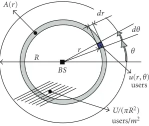
Consider a differential annular zone centered at the base station (Figure 3) with an internal (resp., external) radius ofr (resp.,r +dr). We denote this annular zone by A(r). The area of A(r) is π(r+dr)2 − πr2 _{2πrdr. When}

U users are uniformly distributed over the cell of radius

R, we have a constant user density of U/(πR2_{). Thus, the} annular zone A(r) contains 2Ur dr/R2 _{users. These users} are uniformly distributed over 2π radians around the base station. This means that the number of users contained within the differential angular sector [θ,θ+dθ] radians at distances in ]r,r+dr] (seeFigure 3) is equal to

u(r,θ)=

2Ur/R2_{dr dθ} 2π =

U

πR2r dr dθ. (50)

Since the shadowing is closely related to the surrounding environment topology, we assume that these u(r,θ) users are subject to the same shadowing realization. In other words, they have the same shadowed distance d(r,θ) =

N(0,σ2_{). The cumulative distribution function ofd(r,θ) is} given by

Fd(r,θ)(y)=Proba

d(r,θ)≤y

=0.5 + 0.5 erf

10 log₁₀(y/r)

σ√2/α

. (51)

Thus, the average ratio of users whose shadowed distances are in ]0,Rq] is

uRq

= 1

U

R

0 2π

0 Proba

d(r,θ)≤Rq

u(r,θ). (52)

Using (50) and (51) we prove in the appendix that

uRq

=1

2

1 + erf C logRq

R

+R 2

q

R2e 1/C2

1−erf C logRq

R +

1

C

,

(53)

whereC =10α/(σ√2 log 10). The productu(·)Urepresents the average cumulative distribution function of the number of users when actual distances are replaced by the shadowed distances. It is the expectation, with respect to the shadowing random process, of Uq defined in (43). This important

theoretical result is confirmed by simulation inSection 8.

6.2. Rate-Outage Average Performance. Thanks to (53), we can now evaluateUout, the average number of users that can never be served (users in rate outage) because their shadowed distances exceed the rangeRQ, given in (41), of the

lowest-order modulation. We have

Uout

RQ

=1−uRQ

U. (54)

Moreover, the average number of users in rate outage versus an arbitrary cutoffdistanceRcut∈[R,RQ] is given by

Uout

Rcut

=1−uRcut

U. (55) As mentioned earlier, the cutoffdistanceRcutprovides a way to tradeoffthe maximum rate-outage probability (40) and the average number of users in rate-outage (55) against the data rate (48) offered to each served user. The effect ofRcutis investigated by simulation inSection 8.

6.3. Average User-Rate and Spectral Efficiency. In order to derive an approximate bound for the average maximum rate

Dmax, we replace in (48) each variableUqby its expectation

as follows:

Dmax= _Z BS

q=1Uq/log2Mq

. (56)

From (53) we get

Uq=

uRq

−uRq−1

U. (57)

What about the average spectral efficiency achieved by our allocation method? Note that the average number of served users is

Usrv=

Z

q=1

Uq. (58)

TheseUsrvusers achieve an aggregate data rate ofUsrvDmax on average using a total bandwidth ofBS. So, from (56) we find that the average spectral efficiency is given by

η=

Z q=1Uq

Z

q=1Uq/log₂Mq

. (59)

Notice that the constraint of the minimum data rate per user

D0has not been considered yet. Considering this additional constraint provides a criterion for admission control as discussed inSection 6.2.

6.4. System Capacity and Admission Control. HavingDmax≥

D0along with (48) and (57) gives the followingupper-bound on the bearable number of users

Umax= BS

D0 Z

q=1

uRq

−uRq−1

/log₂Mq

. (60)

ThisUmaxcorresponds to a kind ofmaximum system loadin terms of number of users given the minimum required QoS. When the system is fully loaded, that is,U=Umax, it cannot offer to each user better than the minimum required data rate

D0. In this case, any additional user that requests an access to the service is rejected by the base station. So, the ratioU/Umax can be considered as a metric for the system load. In brief, for

U≤Umaxwe have

Dmax=Umax

U D0. (61)

Section 7 describes the proposed resource allocation

algo-rithm from a practical point of view.

7. Resource Allocation Algorithm in Practice

In the following we assume that U ≤ Umax. We saw that the optimal user-wise subcarrier allocation is defined by (49). However, one must take into account the fact that, in practice, only an integer number of subcarriers can be assigned to a given modulation zone. Thus, theSq’s have to

be rounded to integer numbers. Let

Sq=I

Sq

=I

Uq/log2Mq

Z

k=1Uk/log2Mk

S

, (62)

whereI(x) is the nearest integer tox. TheseSq’s define Z

zones inside the frame where the first zone, for example, is constituted of slots modulated by the M1-QAM constella-tion.

From (44), the number of subcarriers that a user uin zoneqneeds to achieve the common rate is equal toW(u)=

Su

b

ca

rri

er

in

d

ex

f

1 2 . . . s . . . S

Su

b

ca

rri

er

sp

ac

in

g

B

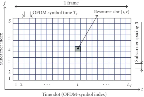
1 frame

OFDM symbol timeTs Resource slot (s,t)

Time slot (OFDM-symbol index)

1 2 · · · t · · · Lf t

Figure4: Frame structure and elementary resource slot.

necessarily an integer. In practice, users are mapped to a frame of lengthLf OFDM symbols (seeFigure 4). WithS

subcarriers, a frame is composed of SLf slots. Let Nq be

the integer number of slots allocated to each user in zone

q. Hence, each user obtains on average Nq/Lf subcarriers

per frame. So, to cope with a nonintegerW(u), the value of

Nqmust be chosen so that the difference|Nq/Lf −W(u)|is

minimized. This gives

Nq=I

LfW(u)

=I

LfDmax

Blog₂Mq

. (63)

The difference betweenNq/LfandW(u) makes the obtained

average data rate per user NqBlog2Mq/Lf slightly different

from the theoretical value Dmax. This difference decreases with the frame length Lf. Moreover, the actual number of

users that can be mapped to theSqLf slots of theMq-QAM

zone in the frame is equal to

Uq=S1÷Nq, (64)

where÷is the integer division operator.

Now we describe the proposed resource allocation algo-rithm. We assume that the shadowed distances of users are known to the base station. So, the base station can sort the users in a vectorUaccording to their increasing shadowed distances. Under these assumptions, the proposed resource allocation algorithm consists of two steps. The first step can be done once of-line while the second needs to be carried out dynamically according to the system load and to the CSI update rate.

Step 1(offline resource reservation).

(1) Find the required power marginFusing (35). (2) Use (34) to find the maximum rangeRqfor eachM

-QAM constellation.

(3) Calculate from (40) the cutoffdistanceRcutthat yields an acceptable maximum rate-outage probability. (4) Deduce the required number of zonesZ from (46)

and the corresponding set of constellations (i.e., the

Zfirst high-order constellations inM).

Step 2(online resource allocation).

(1) Using the vectorUof users sorted according to their shadowed distances, find Uq, the number of users

belonging to each modulation zone.

(2) Deduce the zone-wise number of subcarriersSq for

q=1,. . .,Zusing (62).

(3) Compute the maximum common rate Dmax from (48).

(4) Use (63) and (64) to calculate Nq, the required

number of slots per user as well as the number of bearable usersUq, respectively.

(5) Map users to the frame slots are as follows: the first

U1users inUare mapped to the firstS1subcarriers corresponding to the highest-order modulation zone. The first user is granted the first N1 time slots on the first subcarrier. If N1 > Lf, additional time

slots on the second subcarrier is granted to this user untilN1is reached. Then, the next user is allocated the next time slots and so on. These operations are repeated for the nextU2users in U, that belong to the second modulation zone, and so on until all slots are occupied.

Figure 5 illustrates the online step of the allocation

process.

The available CSI, limited to the users shadowed dis-tances, is implicitly used by the base station during the slot allocation stage in Step2. One should wonder how precise does this CSI need to be? In other words, how the achieved performance can be affected by errors on the CSI? Errors may come from imperfect CSI estimation as well as from quantization noise on the feedback channel. Ideally, users are sorted in vector U according to their shadowed distances. Suppose that we modify the order in U of a subset of users belonging to the same modulation zone. This kind of perturbation has no effect on the expected performance since these users continue to get the same resources. On the contrary, some performance degradation may appear when the CSI errors shift some users from a modulation zone to another. The effect of imperfect CSI is evaluated in the numerical results presented inSection 8.

8. Numerical Results

In Table 2, an example of a typical parameter setting is

provided. We assume that the available constellations are 64-QAM, 16-QAM, QPSK, and BPSK. Concerning the SNR thresholdsγq =βM−1q(b) that correspond to the target BERb for these constellations, we know that for the BPSK, the error probability can be expressed using the error function (38) by

b=0.5 erf(√γBPSK). Thus, we have

γBPSK=

Start

- Sort users according to their equivalrnt distances - Find the zone-wise number of usersUq Calculate - The zone-wise number of subcarriersSq

- The zone-wise number of slots per userNq - The zone-wise bearable number of usersUq Initialize - User indexu=1

- Subcarrier indexs=1 - Time slot indext=1 - Modulation zone indexq=1

- Number of slots already allocated to current usern=0

Allocate slot (s,t) to useruwith modulationMq-QAM s=Sq

t=1

Next useru=u+ 1 n=0

Next constellation q=q+ 1

Next slot t=t+ 1 Next subcarriers=s+ 1

frist slott=1

Update CSI (new frame) n=n+ 1

n=Nq?

t=Lf? u≤Uq?

q≤Z?

Yes No

Yes

No Yes

No

No Yes

Figure5: Flow chart of the resource allocation online step.

For higher-order modulations (Mq>2), a good

approxima-tion of the SNR threshold for anMq-QAM modulation with

b≤10−3is given in [19] by

γq=

Mq−1

Γ(b), (66) whereΓ(b)= −log(5b)/1.6.Table 3gives for each constella-tion the SNR-thresholdγqcorresponding to a BER of 10−3.

In the following, the performance of our allocation method is characterized versus theworst-case average SNR (WASNR) defined by

γwa= PtotG0

SBN0Rα.

(67)

This WASNR corresponds to the area-mean SNR on the cell edge. Given the parameter setting inTable 2, we find using (35) that the required power margin in logarithmic units is FdB = 10 log10F 12.9 dB. In Figure 6 the maximum attainable range (BPSK coverage) for γwa ∈ [5, 25] dB is plotted using (34) and (67). Taking into account the target cell radiusR=100 m, we see that the minimum acceptable WASNR value isγwa19.64 dB (Ptot2.73 W). Moreover, if we assume that the maximum possible value for the total power isPtot = 10 W, we find from (67) thatγwa must be limited to about 25.6 dB. Hence, in the following, we let the WASNR varies in the range [20, 25] dB.

Worst-case (edge-user) average SNR (dB)

5 10 15 20 25

M

axim

u

m

range

(BPSK)

(m)

20 40 60 80 100 120 140 160

Figure 6: Maximum attainable range (BPSK coverage) versus

worst-case (edge-user) average SNR (WASNR).

Shadowed distance (m)

0 50 100 150 200 250 300

N

o

rm

aliz

ed

av

er

age

h

ist

o

gr

am

0 0.005 0.01 0.015 0.02 0.025 0.03 0.035 0.04

Analytic Simulated

Figure7: Average histogram of user shadowed distance.

Let us start by checking the validity of the average shadowed user distribution defined in (53). Remember that the product u(x)U represents the average cumulative dis-tribution function of the number of users whose shadowed distances are within [0,x]. In other words, the average histogram of the shadowed distances must coincide with (u(x + Δx)−u(x))U for Δx 1. This is validated by simulation results depicted inFigure 7where the curves are normalized to the total number of users and averaged on 1000 shadowing realizations.

Table2: Simulation parameters’ values.

Center frequencyfc 3.5 GHz

Total transmit powerPtot 10 W

Number of subcarriersS 256 subcarriers

Total bandwidthBtot 20 MHz

Subcarrier spacingB=Btot/S 78.125 KHz

OFDM symbol durationTs=1/B 12.8 μs

Frame lengthLf 100 symbols

Frame durationLfTs 1.28 ms

Noise power spectral densityN0 −174 dBm/Hz

Path-loss exponentα 3.6 —

Shadowing standard deviationσ 5 dB

Target minimum data rateD0 100 Kbps

Target BERb 10−3 _—

Target maximum outage probabilityε 0.05 —

Target cell radiusR 100 m

Table3: Available modulations’ SNR thresholds forb=10−3_.

Modulation 64-QAM 16-QAM QPSK BPSK

Zone indexq 1 2 3 4

γq(dB) 23.2 17 10 6.8

Rcutis set to the BPSK rangeRBPSK, the maximum number of users is served except those who fall beyondRBPSKin terms of shadowed distance. The achieved data rate is improved in the opposite case when the base station decides not to serve users beyond the cell edge by settingRcut=R. The improvement is significant for high SNRs while it vanishes near SNR=20 dB whereRBPSK R. The gain in user rate is paid for in terms of the average number of users in rate outage as expected by (55). This is shown inFigure 9. So, a tradeoffhas to be found, viaRcut, between user rate and rate outage. By varyingRcut for a fixed total powerPtot=10 W, we show inFigure 10the average percentage of users in rate outage versus the average maximum user rate.

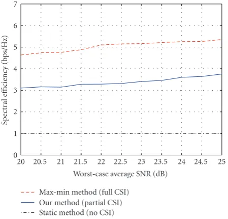
Now we compare the average spectral efficiency (59) of our allocation method to the average spectral efficiency of two other methods. The first one, used if no CSI is available, corresponds to a traditional “static” allocation of subcarriers and rates based on a worst-case design. The second allocation method, called “Max-Min” method, is the one introduced in [7] and reused in [6]. It is based on the assumption of full CSI knowledge that allows an improved spectral efficiency but requires excessive feedback overhead.

In the static allocation case, the power margin must account for both effects of shadowing and fading. We found by simulation that under a composite log-normal-Rayleigh channel, the required power margin for the specified BER and outage probability is F = 14.8 dB. This value can be retrieved analytically using results in [21] where it was shown that a composite log-normal-Rayleigh distribution is equiva-lent to a modified log-normal distribution. Without any CSI, the same modulation must be used over all subcarriers. The

Worst-case (edge-user) average SNR (dB)

20 20.5 21 21.5 22 22.5 23 23.5 24 24.5 25

U

ser

data

ra

te

(Kbps)

0 100 200 300 400 500 600 700 800 900 1000

Analytic Simulated

Rcut=R

Rcut=RBPSK

Figure8: Maximum user rate versus worst-case average SNR for U=100 users.

modulation orderM must guarantee to edge users (worst-case) the required BER. So, M can be obtained by setting

duin (36) to the cell radiusR. Then, theSsubcarriers must

Cut-offdistance (m)

100 105 110 115 120 125 130 135 140

N

u

mb

er

of

users

in

rat

e-outage/numb

er

o

f

u

sers

(%)

0 2 4 6 8 10 12 14 16 18 20

Analytic Simulated

Figure 9: Average percentage of users in rate outage versus the cutoff distance forU = 100 users andPtot = 10 W (WASNR

25 dB).

Achieved user rate (Kbps)

600 650 700 750 800 850 900

P

er

centage

of

users

in

rat

e-outage

(%)

0 2 4 6 8 10 12 14 16 18 20

Rcut=R

Rcut=RBPSK

Figure 10: Tradeoff between the achieved user rate and the

percentage of users in rate outage forU=100 users andPtot=10 W (WASNR25 dB).

120 m (the mid-point between the cell radius and the BPSK range). According to Figure 9, this cutoff distance yields about 8.5% of users in rate-outage. This, from Figure 10, corresponds to an average user rate of 760 kbps. To make the comparison fair, the CSI is quantized on 3 bits. This reduces the feedback overhead required by the “max-min” method to 3Sbits per user. However, our allocation method requirement in terms of CSI precision is significantly less

Worst-case average SNR (dB)

20 20.5 21 21.5 22 22.5 23 23.5 24 24.5 25

Spect

ral

e

ffi

ciency

(bps/Hz)

0 1 2 3 4 5 6 7

Max-min method (full CSI) Our method (partial CSI) Static method (no CSI)

Figure 11: Average spectral efficiency of our allocation method compared to the static and max-min methods forU = 10 users andRcut=120 m.

as shown in the sequel. Due to multiuser diversity gain, the “Max-Min” method exhibits a spectral efficiency gain of about 1 bps/Hz when the number of users passes from 10 to 100. On the otherhand, the average spectral efficiency of our method is unchanged as expected by (59). In both cases, for the static method, the whole cell is covered using the BPSK of spectral efficiency 1 bps/Hz. We see that our allocation method offers a significant spectral efficiency gain compared to the static method.

As mentioned earlier, the main advantages of our method are its simplicity and the limited CSI feedback it requires. The price to be paid is some degradation in spectral efficiency compared to the full-CSI-based “max-min” method as shown in Figures11and12. This loss is compensated by the complexity reduction and the limited feedback overhead that our algorithm requires.

Concerning the rate outage, note that the static method yields zero rate outage at the expense of the achieved spectral efficiency. If the BPSK is replaced by the QPSK, the rate outage remains null (since the BS has not any criterion for rejecting some users) while the BER-outage probability constraint will be violated for near-edge users which is not compatible with the target of this work. The simulated average percentage of users in rate outage is plotted in

Figure 13versus the WASNR and compared to the expected

analytic results from (55).

Finally, we want to characterize the sensitivity of our allocation method to CSI accuracy. Imperfect CSI is modeled by adding a zero-mean Gaussian error to the user shadowed distance. We assume that errors for different users are independent. Thus, if du is the shadowed distance of user

u, the estimated distance is du = du+ eu. The error eu

Worst-case average SNR (dB)

20 20.5 21 21.5 22 22.5 23 23.5 24 24.5 25

Spect

ral

e

ffi

ciency

(bps/Hz)

0 1 2 3 4 5 6 7

Max-min method (full CSI) Our method (partial CSI) Static method (no CSI)

Figure 12: Average spectral efficiency of our allocation method compared to the static and max-min methods forU =100 users andRcut=120 m.

Worst-case average SNR (dB)

20 20.5 21 21.5 22 22.5 23 23.5 24 24.5 25

P

er

centage

of

users

in

rat

e

o

utage

(%)

8 8.5 9 9.5 10 10.5 11 11.5 12 12.5 13

Simulated Analytic

Figure13: Average percentage of users in rate outage versus the worst-case average SNR forU=100 users andRcut=120 m.

thatarepresents the error standard deviation normalized to the cell radiusR. This parameter measures the CSI accuracy (a perfect CSI corresponds toa = 0). Errors on shadowed distances disturb the rate allocation decision leading to unexpected BER outage events. We use theaverage percentage of users in BER-outage per frameas an overall performance metric. InFigure 14, this metric is plotted versus the accuracy parameter a for a fully loaded system (U = Umax) and a total powerPtot = 10 W. We notice that the percentage of users in BER outage for perfect CSI (a = 0) is about 2 %. The degradation does not exceed 2 % even ata=0.5 which corresponds to a significantly-degraded CSI. This shows the robustness of the proposed resource allocation method to

CSI accuracy parametera

0 0.05 0.1 0.15 0.2 0.25 0.3 0.35 0.4 0.45 0.5

A

ver

age

p

er

ce

ntage

o

f

u

sers

in

BER

o

utage

(%)

0 0.5 1 1.5 2 2.5 3 3.5 4 4.5 5

Figure14: Effect of CSI accuracy measured by the parameteraon the average percentage of users in BER outage (U =Umax, Ptot = 10 W).

CSI estimation errors. So, even with coarse estimates of users’ shadowed distances, the achieved overall performance remains acceptable. In fact, all the base station needs in order to properly allocate the resources is the index of the modulation zone each user belongs to. Assume that the base station broadcasts the modulation zones’ radii to all the users in a dedicated frame header and that the shadowed distances are estimated by users themselves. In this case, each user can find the index of his modulation zone and then feedback this value to the base station on the uplink. This fedback information is simply a discrete value between 1 and Z, the number of modulation zones. So, the feedback requires about log₂Z information bits per user. In our example above where Z = 4 zones, two bits per user are needed. This approach is equivalent to quantizing the CSI, or users’ shadowed distances, using irregular thresholds which are the zones radii (Rq =51, 76, 119, 146 (m) in our example). In

full CSI approaches, if the CSI is quantized onNbits, the feedback overhead isNSbits per user.

9. Conclusion

In this paper, we considered the problem of resource allocation on the downlink of a single-cell OFDMA system under QoS fairness constraints with limited channel state information (CSI). Fairness was defined by a minimum user data rate, a target BER, and a maximum BER-outage probability. We supposed that the only CSI available to the base station is a coarse estimation of the users shadowed dis-tances that we defined. Thus, under the fairness constraint, a total peak power constraint and a given number of users uniformly distributed over the cell of a given radius, we derived the optimal subcarrier and rate allocation that offers the maximum data rate per user.