Novel Finite Element Methods for Wave Propagation Modeling

(1)

ABSTRACT

YUE, BIN. Novel Finite Element Methods for Wave Propagation Modeling (Under the direction of Dr. Murthy N. Guddati)

The phenomenon of wave propagation is encountered in various engineering problems related to earthquake engineering, nondestructive evaluation and acoustics. Due to the complex material and geometrical features, many of these wave propagation problems are modeled using numerical methods such as the finite element method. Most numerical methods, due to their approximate nature, incur errors in the solution. In the context of wave propagation, these errors can be classified as amplitude and dispersion errors. Of these, dispersion error tends to have more severe effect on the accuracy due to its accumulative nature. Although it is possible to reduce the dispersion error by mesh refinement, such refinement imposes unrealistic computational cost even for medium-sized problems. In light of this, researchers have long sought efficient methods that reduce the dispersion error without any mesh refinement, but such efforts have only been partially successful. This dissertation develops efficient finite element methods for simulation of time-harmonic as well as transient wave propagation.

(2)

higher convergence rate while maintaining low computational cost. When applied to elastic waves, the modified integration rules can reduce the dispersion error for either longitudinal or transverse wave, but not both.

(3)

Novel Finite Element Methods for Wave Propagation Modeling

by

Bin Yue

A dissertation submitted to the Graduate Faculty of

North Carolina State University

in partial fulfillment of the

requirements for the Degree of

Doctor of Philosophy

Civil Engineering

Raleigh

2004

APPROVED BY:

_________________________

Murthy N. Guddati

(Chair of Advisory Committee)

__ _

Vernon C. Matzen

M. Shamimur Rahman

__ _

(4)

ii

(5)

BIOGRAPHY

(6)

iv

ACKNOWLEDGEMENTS

First and foremost, I want to thank my parents for their unconditional love and support. I am grateful to my doctoral advisor Dr. Murthy Guddati. This dissertation would not exist at all without him. His knowledge, energy, friendship, and inspiration will always serve to me as an example of the perfect supervisor.

Many thanks go to my committee members, Dr. Rahman, Dr. Matzen, Dr. Kumar and Dr. Yuan for helpful discussions and invaluable professional advices.

(7)

List of Tables

(10)

List of Figures

(11)

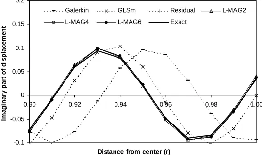
Figure 2-18. Cylindrical radiation problem: displacement in the outermost wavelength of the

computational domain along 0 degree ………... 45

Figure 2-19. Cylindrical radiation problem: displacement in the outermost wavelength of the computational domain along 45 degree ………. 45

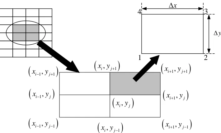
Figure 3-1. Nine-node four-element rectangular finite element patch for dispersion analysis (nine-node stencil in case of finite differences) ………. 60

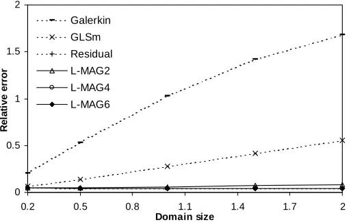
Figure 3-2. Meshes used in numerical examples of plane wave and point source radiation ..65

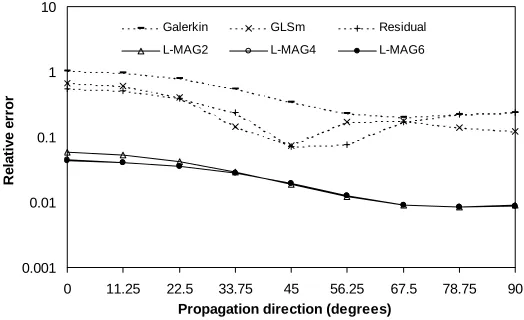
Figure 3-3. Error for varying angles of propagation (with uniform rectangular elements) …65 Figure 3-4. Error for varying domain sizes (with uniform rectangular elements)………….. 66

Figure 3-5. Layout of the distorted mesh (h=0.005) ………...66

Figure 3-6. Error for varying angles of propagation (with distorted rectangular elements)…67 Figure 3-7. Error for varying domain sizes (with distorted rectangular elements) ………… 67

Figure 3-8. Radiation from point source (with uniform rectangular elements): Response along the radius………..68

Figure 3-9. Radiation from point source (with distorted rectangular elements): Response along the radius ……….. 68

Figure 3-10. Radiation from an infinitely long circular cylinder: Finite element mesh …….70

Figure 3-11. Radiation from an infinitely long circular cylinder: Response along the radius.70 Figure 4-1. Dispersion relations of Galerkin method and Modified integration rules ………77

Figure 4-2. Incident, reflected and transmitted waves ………78

Figure 4-3. Error for varying angles of incident waves ………..79

Figure 4-4. Point load on a layered half-space ……….. 80

Figure 5-1: Four-element nine-node finite element patch ………. 95

(12)

Figure 5-4: Displacement contours for the Gaussian explosion example ……… 110

Figure 5-5: Displacement variations for the Gaussian explosion example ……….. 111

Figure 5-6: The unstructured finite element mesh ………... 112

(13)

1 Introduction

1.1 Numerical Modeling of Wave Propagation

The phenomenon of wave propagation is encountered in several engineering problems of

immense socio-economic impact. Some of such problems are related to nondestructive

evaluation (NDE), earthquake engineering and medical imaging. In several NDE techniques,

acoustic and electromagnetic wave scattering is used to detect damage, flaws and cracks and thus

predict the serviceability of vital structures [1]. In earthquake engineering, the response of the

structure to the impinging seismic waves depends on the complicated dynamic interaction

between the structure and the soil [2]. Medical imaging is similar to NDE in that the tissue

characteristics are determined by examining the scattering of waves [3]. Similar imaging

techniques are being used to detect landmines for both military and humanitarian purposes [4].

Most of the real life problems described above involve complicated material and geometrical

features. For example, in the context of nondestructive evaluation of composite structures, it is

important to understand propagation, scattering and attenuation of waves in complex

heterogeneous media. Modeling such phenomena is not possible through analytical methods,

and is often performed through numerical simulations. Among all the numerical methods (Finite

Difference Method (FDM), Finite Element Method (FEM), Boundary Element Method (BEM),

Spectral Method [5], Pseudo-spectral Method [6], Wavelet-based Method [7], Mass-Spring

Lattice model [8]), FEM is most appealing for solving wave propagation problems involving

(14)

Due to the approximate nature of the numerical methods, these simulations result in

solution errors in the form of artificial distortion, dissipation and reflection of waves. It is

possible to reduce these numerical errors by simply refining the discretization in space and time.

However, such refinement imposes significant increase in computational cost. For example, a

simulation of 40 seconds of an aftershock from the 1994 Northridge quake in Southern

California runs for 6.5 hours on 256 processors of a Cray T3D [9]. A posteriori error estimation

could be used to dynamically change the discretizations in space and/or time [10-12]. Such

adaptive methods are often taxed with huge computational efforts associated with re-meshing.

Improved computational methods producing accurate solutions without requiring fine

meshes could help overcome this limitation. Developing such efficient methods is the focus of

this dissertation.

1.2 Preliminaries

Following is a brief discussion of linear wave propagation in elastic and acoustic media.

Further discussion of wave phenomena can be found in many books (e.g. [13], [14], [15]). Essentially, the governing differential equation of the motion of a mechanical system is obtained

by combining (a) balance of linear momentum, (b) strain-displacement relationships and (c)

constitutive laws.

The balance of linear momentum gives rise to

2 2 t

ρ∂ − ∇ ⋅ = ∂

u

σ f, (1)

(15)

The constitutive relationship for isotropic linear elasticity is given by

( )

2

trace λ G

= +

σ ε I ε, (2)

where is the identity tensor, I λ and G are the Lame constants of elasticity, and is the infinitesimal strain tensor defined in (3).

ε

The strain is defined as the symmetric part of the gradient of the displacement

[ ]

symm

= ∇

ε u . (3)

Using the above three equations and further simplification, we arrive at the elastic wave

equation

(

)

(

)

(

)

2

2 2G G

t

ρ∂ − ∇ λ+ ∇ ⋅ + ∇× ∇× =

∂

u

u u f. (4)

Alternatively, the constitutive equation is usually expressed as

=

σ Dε, (5)

where is a fourth order tensor made up of Young’s modulus and Poisson’s ratio D E µ. The elastic wave equation is thus expressed as

(

)

2 2 t

ρ∂ − ∇ ⋅ ∇ = ∂

u

D u f . (6)

This dissertation focuses on 2-D waves, while the methods developed here can be easily

extended to 3-D problems.

1.2.1 2-D Elastic Waves (Plane Strain)

Since the tensors are all symmetric for normal materials, they are often expressed in a

simpler way. For example, σ and ε are expressed as vectors and as a second order tensor. In this way, the governing differential equation is written as follows,

(16)

2 2 T t ρ∂ − + ∂ u

L σ =f , (7)

=

σ Dε, (8)

=

ε Lu, (9)

where,

0

, , , 0

x x x y y y xy xy x u u y x y σ ε σ ε τ ε ⎡ _∂ ⎤ ⎢ ⎥ ∂ ⎢ ⎥ ⎡ ⎤ ⎡ ⎤ ⎡ ⎤ ⎢ ∂ ⎥ ⎢ ⎥ ⎢ ⎥ =_{⎢ ⎥} =_{⎢ ⎥} =_{⎢ ⎥} =_⎢ _⎥ ∂ ⎣ ⎦ _⎢ _⎥ ⎢ ⎥ ⎢ ⎥ ⎣ ⎦ ⎣ ⎦ _⎢_∂ _∂ _⎥ ⎢_∂ _∂ ⎥ ⎢ ⎥ ⎣ ⎦

σ ε u L (10)

and is expressed in terms of and D E µ. The problem statement is then,

(

)

22

T t ρ∂ − + ∂ u

L DLu =f (11)

with boundary conditions

(

)

( )

hg

t on

⋅ = Γ

= Γ

DLu n h

u g (12)

and initial conditions

( )

0 0 at t at t t = = ∂ ₌ ₌ ∂ 0 0

u u x u

v x (13)

1.2.2 Time Harmonic Plane Strain Elastic Wave

When the forcing function and boundary conditions are time harmonic, i.e.

i t i t i t

e−ω e−ω e

= = =

(17)

then (11) becomes the reduced wave equation,

(

)

2

T ρω

−L DLU − U F= , (15)

(

)

h

g

on on

⋅ = Γ

= Γ

DLU n H

U G (16)

1.2.3 Anti-plane Shear Waves

For anti-plane shear, the displacement is scalar, and the governing equation takes the form

(

)

22

T u

D u f

t

ρ∂

− + =

∂

L L , (17)

where

x

y ∂ ⎡ ⎤ ⎢ ⎥_∂ ⎢ ⎥ =

∂ ⎢ ⎥ ⎢ ⎥_∂ ⎣ ⎦

L (18)

with boundary and initial conditions

(

)

( )

gh

D u = h t on

u g t on

⋅ Γ

= Γ

L n

(19)

( )

0 0

0

u u at t

u

= v at t

t

= =

∂

= ∂

x

x (20)

1.2.4 Time Harmonic Scalar Wave Equation (Helmholtz Equation)

When the forcing function and boundary conditions are time harmonic, i.e.

-iwt -iwt -iwt

(18)

(

)

2 T

D U ρω U F

−L L − = (22)

(

)

h

g

D U H on

U G on

⋅ = Γ

= Γ

L n

(23)

1.3 Background and Objectives

1.3.1 Time Harmonic Analysis

When standard (Galerkin) finite element method is used for simulating time-harmonic wave

propagation, two types of numerical errors occur - error in amplitude and error in wavelength

[17, 18]. In large-scale simulations where the domain size is much larger than the wavelength, the error in the wavelength, known as the dispersion error, tends to accumulate and produce

large phase errors, resulting in completely erroneous results [19]. On the other hand, amplitude

error is relatively benign in that it does not increase with growing domain size. For this reason,

the dispersion error has received increasing attention in the past twenty to thirty years.

It can be quickly realized that dispersion error in one-dimensional time harmonic problems

can be completely eliminated by resorting to analytical solutions [19]. For higher dimensions,

the dispersion error cannot be completely eliminated [20], but can be reduced. Over the past

two decades, several researchers have proposed various methods for reducing the dispersion in

higher dimensions. Following is a brief survey.

The peculiar aspect of dispersion error in higher dimensions is its anisotropy, i.e. the

dispersion error depends on the angle between the wave propagation direction and mesh

orientation. Researchers analyzed this property almost twenty years ago [18], and proposed

(19)

for specific cases, but lose their accuracy in more general cases. More recently, Harari and

Hughes [21] have used mathematically precise Galerkin/least squares (GLS) method [22] to reduce dispersion on square meshes. The resulting dispersion error, although reduced, is still

significant. Thompson and Pinsky [23] modified this method to further reduce the dispersion,

but their method still suffers from anisotropy. Babuska and Ihlenburg [24] used the concepts of

Generalized FEM and finite difference stencils to derive a method that reduces the dispersion by

several orders of magnitude, but only for square meshes. Oberai and Pinsky [25] used the

concept of edge residuals to derive the same scheme in the context of finite elements. Their

scheme, when extended to rectangular or unstructured meshes, becomes heuristic in nature and

loses its accuracy properties. Babuska and Melenk [26] used a partition of unity method to

reduce the dispersion, but its practicality is severely limited in that one needs to know the

behavior of the solution a-priori, which is often not the case. Other efforts to reduce the error in

time-harmonic finite element analysis include [27], [28], [29] and [30].

A fundamental limitation of all the above methods is that they are applicable only for

propagating waves in homogeneous media discretized by regular meshes. Many important and

practical problems of wave propagation involve complex geometries and material

heterogeneities, and cannot be discretized using regular meshes. Furthermore, all the above

methods have been developed for acoustics, and the more complicated case of elastic wave

propagation cannot be handled by the above methods. The modified Galerkin/gradient least

square method [31] is applicable to elastic wave propagation, but has anisotropic dispersion

error and cannot handle non-uniform and unstructured meshes.

(20)

increases the accuracy of wave propagation modeling. Thus the first objective of this dissertation

is to obtain increased accuracy finite element methods for time-harmonic wave propagation,

requiring minimal increase in the computational cost.

1.3.2 Transient Analysis

Wave propagation in the time domain is generally performed by finite element and finite

difference methods, in conjunction with time stepping algorithms. In addition to the spatial

dispersion error discussed in the previous section, such simulations result in temporal dispersion

(error in time-period) and dissipation (decay of amplitude). These errors are affected by the

choice of the spatial discretization as well as the choice of the time integration algorithm. An

analysis of time stepping algorithms and their influence on temporal dispersion and dissipation

in structural dynamics problems can be found in [16]. Wave propagation is different from

structural dynamics in that the temporal and spatial discretizations need to be closely coupled to

obtain accurate results. An analysis of combinations of spatial and temporal discretizations for

wave propagation can be found in [32].

Temporal dispersion control has been studied as early as 1973 by Krieg and Key [33]. They

realized the opposing effect of lumped and consistent mass matrices and suggested matching the

mass computation with time stepping algorithm. However, their method is robust only for

uniform one-dimensional meshes, and looses its accuracy when applied to non-uniform meshes,

heterogeneous media, or higher dimensions [16]. A simple analysis will indicate that these

shortcomings are closely related to the anisotropy of the spatial dispersion error discussed in the

previous section. Taylor-Galerkin schemes combined with higher order spatial discretization can

(21)

cost and often require smooth wave fronts. Space-time discretizations [35] and spectral methods

may reduce these errors, but they too are computationally expensive.

Wang et al. [36] obtained a semi-empirical method based on a 1-D analysis and apply it on

both 1-D and 2-D problems. Krenk introduced a local spatial averaging of the velocity [37].

Stolle [38] and Xie [39] used a direct integration algorithm different from the commonly used Newmark family. In the work by Liu et al. [40], the effect of distortional change of element

shape on wave motion is studied. Despite those efforts, existing algorithms that solve transient

wave propagation problems are not satisfactory; they are either expensive or not very accurate.

The second objective of the research is to develop a numerical method to systematically

reduce spatial and temporal dispersion errors for finite element methods combined with various

time stepping schemes.

1.4 Organization

The dissertation is divided into several chapters, each presenting a significant development.

The chapters constitute individual papers/notes. They are either published, in revision, or to be

submitted in the near future.

Chapter 2 describes the first development of the dissertation, namely the local mesh

dependent Galerkin (L-MAG) method. L-MAG method successfully reduces the dispersion

error for acoustic time-harmonic analysis on square and rectangular meshes and has superior

accuracy and flexibility in comparison with the existing methods.

Chapter 3 contains another, much simpler, dispersion reduction technique. Based on

(22)

effective for unstructured meshes. Specifically, the dispersion error is fourth order as opposed to

second order convergence associated with existing methods.

Chapter 4 explores the usage of modified integration rules to evanescent and elastic waves. It

effectively increases the accuracy for the simulation of acoustic wave in heterogeneous media.

When applied to elastic waves, modified integration rules turn out to be not very effective as

they can reduce the dispersion error for either longitudinal or transverse waves, but not both.

Chapter 5 successfully develops algorithms that make the simulation of transient acoustic

waves more efficient, for both implicit and explicit time stepping schemes. The fourth order

convergence rate is again obtained, as opposed to the second order convergence associated with

existing methods.

The final chapter contains some closing remarks on L-MAG method and modified

integration rules, along with some recommendations for future research.

References

1. L. Cartz, Nondestructive Testing (ASM International, Materials Park, OH, 1995).

2. J.P. Wolf, Soil-Structure Interaction Analysis in Time Domain (Prentice Hall, Englewood

Cliffs, NJ, 1988).

3. F.W. Kremkau, Diagnostic Ultrasound: Principles and Instruments (W.B.Saunders,

Philadelphia, PA, 1998).

4. R. Voles, in: Second International Conference on the Detection of Abandoned

Landmines, (1998)

5. D. Komatitsch and J. Tromp, Introduction to the Spectral Element Method for

(23)

6. M. Lou and J.A. Rial, Modelling Elastic-Wave Propagation in Inhomogeneous

Anisotropic Media by the Pseudo-Spectral Method, Geophysics Journal International, 120

(1995) 60-72.

7. T.K. Hong and B.L.N. Kennett, A Wavelet-based Method for Simulation of

Two-Dimensional Elastic Wave Propagation, Geophysics Journal International, 150 (2002) 610-638.

8. H. Yim and Y. Sohn, Numerical Simulation and Visualization of Elastic Waves Using

Mass-Spring Lattice Model, IEEE Transactions on Ultrasonics, Ferroelectrics, and Frequency

Control, 47 (2000) 549-558.

9. H. Bao, J. Bielak, O. Ghattas, L.F. Kallivokas, and D.R. O'Hallaron, Large-scale

Simulation of Elastic Wave Propagation in Heterogeneous Media on Parallel Computers,

Computer Methods in Applied Mechanics and Engineering, 152 (1998) 85-102.

10. C.K. Choi and H.J. Chung, An Adaptive Control of Spatial-Temporal Discretization

Error in Finite Element Analysis of Dynamic Problems, Structural Engineering and Mechanics,

3 (1995) 391-410.

11. C.K. Choi and H.J. Chung, Error Estimates and Adaptive Time Stepping for Various

Direct Time Integration Methods, Computers and Structures, 60 (1996) 923-944.

12. C.A. Issa, K. Balasubramaniam, and K. Srirengan, Adaptive hp-Finite Element for

Transient Analysis, Applied Mathematics and Computation, 65 (1994) 315-334.

13. J.B. Whitham, Linear and Nonlinear waves (John Wiley and Sons, New York, 1974).

14. A. Bedford and D.S. Drumheller, Introduction to Elastic Wave Propagation (John Wiley

and Sons Ltd., Chichester, 1994).

15. J.D. Achenbach, Wave Propagation in Elastic Solids (North-Holland Publishing

(24)

16. T.J.R. Hughes, The Finite Element Method: Linear Static and Dynamic Finite Element

Analysis (Dover, Mineola, NY, 2000).

17. Z.P. Bazant, Spurious Reflection of Elastic Waves in Nonuniform Finite Element Grids,

18. R. Mullen and T. Belytschko, Dispersion Analysis of Finite Element Semidiscretizations

of the Two-Dimensional Wave Equation, International Journal for Numerical Methods in

Engineering, 18 (1982) 11-29.

19. F. Ihlenburg, Finite Element Analysis of Acoustic Scattering. Applied Mathematical

Sciences. Vol. 132 (Springer-Verlag, New York, 1998).

20. I.M. Babuska and S.A. Sauter, Is the Pollution Effect of the FEM Avoidable for the

Helmholtz Equation Considering High Wave Numbers?, S.I.A.M Journal on Numerical

Analysis, 34 (1997) 2392-2423.

21. I. Harari and T.J.R. Hughes, Galerkin/Least Squares Finite Element Method for the

Reduced Wave Equation with Non-reflecting Boundary Conditions, Computer Methods in

Applied Mechanics and Engineering, 98 (1992) 411-454.

22. T.J.R. Hughes, Multiscale Phenomena: Green's Functions, the Dirichlet-to-Neumann

Formulation, Subgrid Scale Models, Bubbles, and the Origins of Stabilized Methods, Computer

Methods in Applied Mechanics and Engineering, 127 (1995) 387-401.

23. L.L. Thompson and P.M. Pinsky, A Galerkin Least-Squares Finite Element Method for

the Two-Dimensional Helmholtz Equation, International Journal for Numerical Methods in

(25)

24. I.M. Babuska and F. Ihlenburg, A Generalized Finite Element Method for Solving the

Helmholtz Equation in Two-Dimensions with Minimal Pollution, Computer Methods in

Applied Mechanics and Engineering, 128 (1995) 325-359.

25. A.A. Oberai and P.M. Pinsky, A Multiscale Finite Element Method for the Helmholtz

Equation, Computer Methods in Applied Mechanics and Engineering, 154 (1998) 281-297.

26. I.M. Babuska and J.M. Melenk, The Partition of Unity Finite Element Method,

International Journal for Numerical Methods in Engineering, 40 (1997) 727-758.

27. L.P. Franca, C. Farhat, A.P. Macedo, and M. Lesoinne, Residule-free Bubbles for the

Helmholtz Equation, International Journal for Numerical Methods in Engineering, 40 (1997)

4003-4009.

28. H.P. Cherukuri, Dispersion Analysis of Numerical Approximations to Plane Wave

Motions in An Isotropic Elastic Solid, Computational Mechanics, 25 (2000) 317-328.

29. A. Deraemaeker, I.M. Babuska, and P. Bouillard, Dispersion and Pollution of the FEM

Solution for the Helmholtz Equation in One, Two and Three Dimensions, International Journal

for Numerical Methods in Engineering, 46 (1999) 471-499.

30. L. Jiang and R.J. Rogers, Effects of Spatial Discretization on Dispersion and Spurious

Oscillations in Elastic Wave Propagation, International Journal for Numerical Methods in

Engineering, 29 (1990) 1205-1218.

31. I. Harari and S. Haham, Improved Finite Element Methods for Elastic Waves,

32. K.J. Marfurt, Accuracy of Finite Difference and Finite Element Modeling of the Scalar

(26)

33. R.D. Krieg and S.W. Key, Transient Shell Response by Numerical Time Integration,

International Journal for Numerical Methods in Engineering, 7 (1973) 273-286.

34. A. Safjan and J.T. Oden, High-Order Taylor-Galerkin and Adaptive hp-Methods for

Linear Hyperbolic Systems, Journal of Computational Physics, 120 (1995) 206-230.

35. T.J.R. Hughes and G.M. Hulber, Space-time Finite Element Methods for

Elastodynamics: Formulation and Error Estimates, Computer Methods in Applied Mechanics

and Engineering, 66 (1988) 339-363.

36. Y.C. Wang, V. Murti, and S. Valliappan, Assessment of the Accuracy of the Newmark

Method in Transient Analysis of Wave Propagation Problems, Earthquake Engineering and

Structural Dynamics, 21 (1992) 987-1004.

37. S. Krenk, Dispersion-corrected Explicit Integration of the Wave Equation, Computer

Methods in Applied Mechanics and Engineering, 191 (2001) 975-987.

38. D. Stolle, A Direct Integration Algorithm and the Consequence of Numerical Stability,

Journal of Sound and Vibration, 180 (1995) 513-518.

39. Y.M. Xie, An Unusual Stability Property of A Direct Integration Algorithm, Journal of

Sound and Vibration, 192 (1996) 1015-1017.

40. J.B. Liu, S.K. Sharan, and L. Yao, Wave Motion and Its Dispersive Properties in A Finite

(27)

2 Local Mesh-dependent

Augmented Galerkin Methods for

Reducing Dispersion Error for Helmholtz Equation

Abstract

Finite element solution of time-harmonic wave propagation results in numerical dispersion that sometimes translates into completely erroneous results, especially for large-scale problems. This paper presents a new framework for developing reduced dispersion finite element methods. Based on the idea of adding element level mesh-dependent parameters to the original Galerkin FEM, hence called the local mesh-dependent augmented Galerkin (L-MAG) method, the proposed method effectively reduces the anisotropic numerical dispersion occurring in multi-dimensional wave propagation simulations. The computational cost of L-MAG FEM is almost identical to Galerkin FEM. With respect to accuracy, while the existing dispersion reducing methods are largely limited to uniform meshes with square elements, the L-MAG FEM, due to its local nature, is able to significantly reduce the numerical dispersion on non-uniform meshes with rectangular elements. This paper contains the formulation of L-MAG FEM, an analysis of associated dispersion errors, and numerical examples that illustrate the method’s effectiveness. [In revision for International Journal for Numerical Methods in Engineering]

2.1 Introduction

Numerical techniques for analyzing wave propagation have been developed by various

researchers over the latter half of the past century. These include finite difference methods,

finite element methods, boundary element methods, spectral methods and other specialized

methods. Of these, finite element methods (FEM), due to their flexibility, appear most appealing

for solving problems involving complex geometry and material heterogeneities. Due to their

approximate nature, FEM and other numerical methods incur errors in the solution. In

(28)

wave propagation, two types of numerical errors occur – error in amplitude and error in

wavelength [1, 2]. In large-scale simulations where the domain size is much larger than the

wavelength, the error in the wavelength – known as the dispersion error – tends to accumulate

and produce large phase errors, resulting in completely erroneous results [3]. On the other hand,

amplitude error is relatively benign in that it does not increase with growing domain size. For

this reason, the dispersion error has received increased attention in the past twenty to thirty

years.

The dispersion error could simply be reduced either by using a finer mesh, or by using

higher order finite elements. Both of these options come with large increase in computational

cost, making some of the large-scale simulations prohibitively expensive. Thus, if possible, it is

desirable to reduce the dispersion error without significantly increasing the computational cost.

It can be quickly realized that dispersion error in one-dimensional problems can be completely

eliminated by resorting to analytical solutions [3]. For higher dimensions, the dispersion error

cannot be completely eliminated [4], but can only be reduced. Over the past two decades,

several researchers have proposed various methods for reducing the dispersion in higher

dimensions. Following is a brief survey.

The peculiar aspect of dispersion error in higher dimensions is its anisotropy, i.e., the

dispersion error depends on the angle between the wave propagation direction and mesh

orientation. Mullen and Belytchko [2] have analyzed this property, and proposed some ad-hoc

methods to reduce the dispersion on uniform meshes. These methods work well for specific

cases, but lose their accuracy in more general cases. More recently, Harari and Hughes [5] have

used mathematically precise Galerkin/least squares (GLS) method [6] to reduce dispersion on

(29)

and Pinsky [7] modified this method to further reduce the dispersion, but their method still

suffers from anisotropy. Babuska, Ihlenburg et al. [8] used the concepts of Generalized FEM

and finite difference stencils to derive a method that reduces the dispersion by several orders of

magnitude, but only for square meshes. Oberai and Pinsky [9] used the concept of edge

residuals to derive the same scheme in the context of finite elements. Their scheme, when

extended to rectangular or unstructured meshes, becomes heuristic in nature and loses its

accuracy properties. Babuska and Melenk [10] used a partition of unity method to reduce the

dispersion, but its practicality is severely limited in that one needs to know the behavior of the

solution a-priori, which is often not the case. The method of Residual free bubbles, developed

by Franca, Farhat et al. [11], is a robust method that can improve the accuracy by effective

enrichment of shape functions, but such enrichment demands significant increase in

computational cost, especially for non-uniform meshes. Similar comment applies to the sub-grid

modeling approach proposed by Cipolla [12]. Other contributions include Lee and Cangellaris

[13], Scott [14], Harari [15], Ihlenburg [16], Deraemaeker et al. [17] and Rao et al. [18].

A fundamental limitation of all the above methods is that they are applicable only for

propagating waves in homogeneous media discretized by regular meshes. Many important and

practical problems of wave propagation involve complex geometries and material

heterogeneities, and cannot be discretized using regular meshes. Although dispersion reducing

methods for triangular meshes may offer added flexibility [19], the current versions are limited to

uniform structured meshes.

In this paper, a new dispersion reducing finite element method is proposed. Based on a new

local mesh-dependent augmented Galerkin (L-MAG) framework, the proposed method reduces

(30)

proposed method is applicable to non-uniform rectangular meshes, and due to its local nature,

shows promise for extension to completely unstructured meshes. This paper focuses on the

development, implementation and testing of the new dispersion reducing methods, with focus

on non-uniform rectangular meshes.

The outline of the paper is as follows: Section 2 contains discussion of the variational

boundary value problem and the (standard) Galerkin finite element discretization of the

problem. In section 3, dispersion error analysis for rectangular meshes is reviewed.

Mesh-dependent augmented Galerkin (MAG) framework is discussed in section 4. This section also

contains the analysis of some existing methods that fit into the MAG framework. In section 5,

the proposed Local MAG (L-MAG) finite element framework is developed and its dispersion

error is analyzed. Subsequent design of dispersion reducing methods based on the L-MAG

framework is presented in Section 6. Section 7 contains the aspects of implementation and

computational cost, whereas section 8 contains several numerical examples illustrating the

effectiveness of L-MAG methods. Concluding remarks are given in section 9.

2.2 Finite Element Method for Time-Harmonic Wave Propagation

Problems

Helmholtz equation, or the reduced wave equation, is used to analyze scalar wave

propagation encountered in linear acoustic and anti-plane shear problems. The corresponding

boundary value problem takes the form: Find u:Ω → , such that

in f u k u− = ∇

− 2 2 Ω

, (1)

on _g

(31)

( )

on _h

u b u F

∇ ⋅ +n = Γ . (3)

In the above, is the complex-valued field variable (acoustic pressure, or anti-plane

displacement), is the wave number associated with the excitation frequency u

k

(

k =ω c

)

, is

the specified field variable on the Dirichlet boundary

g

Γ , whereas a Robin type boundary

condition is specified on the remainder of the boundaryΓh. Here, b is an operator ranging

from zero (for pure Neumann boundary condition) to the DtN map in the context of absorbing

boundaries.

Using classical variational calculus, the above (strong) form of the boundary value problem

can be converted to the following (weak) variational form: Find u:Ω → , with u=g on Γ_g, such that

(

)

2

( ) (

)

(

) (

)

g

, , , ( ) , , , , 0 on

h h

v u k v u v b u _Γ v f v F _Γ v v

∇ ∇ − + = + ∀ = Γ (4)

The notation

( )

i i, is used to define inner product (over the domain Ω) as follows:

(

)

*

,

f g f g d

Ω

=

_∫

Ω, (5)

where the *

f is the complex conjugate of f . The notation

( )

, h

Γ

i i represents inner product

taken over the boundary Γh.

For numerical solution of the above variational boundary value problem, (Bubnov) Galerkin

Finite Element Method (FEM) can be used, where the Galerkin approximation of the variational

boundary value problem takes the form: Find uh:Ω → , with uh =gh on Γg, such that

(

) (

2

) (

)

g

, , , ( ) , , , , 0 on

h h

h h h h h h h h h h

v u k v u v b u v f v F v v

Γ Γ

(32)

In the above, and are approximations of u and respectively, and is the

consistent approximation of the Dirichlet data. In the context of conventional finite element

method, and take the form:

h

u vh v gh

h

u vh

, (7) ( ) ( ) and ( ) ( )

h h

u x =N x U v x =N x V

where is the shape function vector, while Uis the discretized field variable (degree of freedom vector) and is its variation. By substituting (7) in (6), we obtain the algebraic

equation ( ) N x

V

Gal =

S U F, (8)

where _SGalis the coefficient matrix (associated with standard Galerkin method):

(

)

2

(

) (

)

, , , (

h Gal

k ) _Γ

= ∇ ∇ − +

S N N N N N B N , (9)

and is the force vector: F

(

,

) (

,

)

h

f F _Γ

= +

F N N . (10)

In (9), note that is the discretized version of the operator in (3). B b

Due to the approximate nature of Galerkin FEM, errors are incurred in the solution.

Considering that the exact solution for the Helmholtz equation is oscillatory, these errors can be

quantified in terms of amplitude error and the dispersion error (error in wavelength). In

contrast with the amplitude error, dispersion error in each wave cycle accumulates to result in

large phase errors. This is a significant concern especially for large-scale wave propagation

problems where the domain size is several orders of magnitude larger than the wavelength.

Thus, it is desirable to reduce the dispersion error to a small value. First step in obtaining such

a dispersion reduction technique is to perform a quantitative analysis of the dispersion error for

(33)

element meshes, which is a modified version of the analysis for square meshes by used by

Ihlenburg [3] and others.

2.3 Dispersion Error Analysis on Rectangular Meshes

Consider a uniform mesh of rectangular finite elements shown in Figure 2-1. The

coefficient matrix for a four-node rectangular finite element would be:

0 0

x xy y

x y

element

xy y x

y xy x

S S S S

xy

⎡ ⎤

⎢ ⎥

=_⎢ _⎥

⎢ ⎥

⎣ ⎦

S . (11)

The reasons for the above form are as follows: (a) The stiffness matrix is symmetric

since the operator in (9) is self-adjoint. (b) Due to the geometric symmetry of the element, we

can observe the following equalities (the subscripts 0,

(

Sij =Sji

)

,

x y and xy have obvious geometrical interpretations): S11=S22 =S33 =S44 =S0, S12 =S34 =Sx, S13 =S24 =Sxy, .

These observations apply not only to the Galerkin FEM but also to any other modification. In

order to obtain the equations associated with the central node

14 = 23 =Sy

S S

( , )x y of the finite element patch in Figure 2-1, we need to assemble all the four elements connected to the node. Such an

assembly will result in the following form of the equation:

(

)

(

)

(

)

0 , , , , ,

, , , ,

4 2 2

0

h h h h h

x y x x x y x x y y x y y x y y

h h h h

xy x x y y x x y y x x y y x x y y

S u S u u S u u

S u u u u

−∆ +∆ −∆ +∆

−∆ −∆ +∆ −∆ +∆ +∆ −∆ +∆

+ + + +

(34)

Figure 2-1. Nine-node four-element rectangular finite element patch for dispersion analysis (nine-node stencil in case of finite differences)

x ∆

1 2

3 4

(

xi+1,yj

)

(

xi+1,yj−1

)

(

xi+1,yj+1

)

(

xi−1,yj+1

)

(

xi−1,yj−1

)

(

xi−1,yj

)

(

x y_i, _j

)

(

x yi, j+1

)

y

∆

(

x yi, j−1

)

This equation can also be obtained by an equivalent finite difference method using a nine-node

stencil shown in the Figure 2-1. Noting that (12) is applicable for all nodes of the discretized

system, it can be shown that the solution for the difference equations takes the form of a plane

wave:

( cos cos h

ik x y h

u =e θ+ θ) (13)

The only difference between the approximate solution and the exact solution

is that the wave numbers and are different. In fact, the dispersion error can be quantified

as the error in the wave wavelengths:

( )

(

ik xcos ysin

)

u=e θ+ θ

h

k k

2 2

absolute h

dispersion h

e

k k

π π

λ λ

= − = − . (14)

(35)

h h relative dispersion h k k e k λ λ λ − −

= = . (15)

In the above equations, the approximate wave number can be obtained by substituting

the approximate waveform in (13) into the difference equation (12). Such substitution, after

some simplification, results in:

h k

0 x x y y xy x y x y 0 S S C S C S C C u

⎡ + + + ⎤ _, =

⎣ ⎦ , (16)

where,

(

)

(

)

cos h cos and cos sin

x y

C = k ∆x θ C = kh∆y θ . (17)

The expression in the brackets in (16) must be zero for the non-trivial solution

(

. Thus

the discrete dispersion relationship relating the exact and approximate wave numbers is given by:

)

, 0 x y u ≠

0 x x y y xy x y 0

S +S C +S C +S C C = . (18)

For Galerkin method, the elements in the coefficient matrix (11) are:

2 2 2

0

2 2 2

, 3 9 2 , 6 1 2 , 6 1 . 6 3 x y xy 8 8 6

x y k x y

S

x y

x y k x y

S

x y

y x k x y

S

x y

x y k x y

S x y ∆ + ∆ ∆ ∆ = − ∆ ∆ ∆ − ∆ ∆ ∆ = − ∆ ∆ ∆ − ∆ ∆ ∆ = − ∆ ∆ ∆ + ∆ ∆ ∆ = − − ∆ ∆ (19)

The resulting dispersion relation for the Galerkin FEM is:

(

)(

2 2

)

(

2 2

)

(

2 2

) (

)

2 2 2

(36)

Using (20), we can obtain a relation between the exact wave and the approximated wave

number :

k

h k

(

)

(

2 2

)

(

2 2

)

(

2 2

)

12 6 6 2 6 2

1

4 2 2

x y x y

C C x y C x y C y x

k

x y C C C C

− ∆ + ∆ + ∆ − ∆ + ∆ − ∆

=

∆ ∆ + + + . (21)

To evaluate the order of difference between and , we take Taylor expansion of in

terms of (note that and are functions of ),

kh khh k

h

k C_x C_y kh

( )

3

(

( )

5

(

)

4

)

2 4 2 4

1

cos sin

24

h h

k=k + _⎣⎡∆x θ + ∆y θ_⎦⎤ k +O kh ∆ + ∆x y . (22)

The relative dispersion error is given by:

( )

2

₍

₎

4

2 4 2 4

cos sin 24 h h h h k k k

x y O k x

k θ θ

− ₌ _∆ _{+ ∆} ₊ _{∆ + ∆}

₎

y . (23)

Noting that h, we have k ≈k

(

2

4

2 4 2 4 4

cos sin 24

h

k k k

₎

)

x y O k x

k θ θ

− ₌ _∆ _{+ ∆} ₊ _{∆ + ∆}

y . (24)

For square meshes where ∆ = ∆ =x y h, the dispersion error is give by:

( )

2

₍

_{( )}

4 3 cos 4

96 h h kh k k O kh k θ −

= + +

)

. (25)

For lumped mass matrix, the dispersion errors associated with standard Galerkin method

can be obtained using a similar procedure and are given in Table 2-1.

2.4 Mesh Dependent Augmented Galerkin Methods

Many of the methods proposed for dispersion reduction attempt to solve a modification of

(37)

(

) (

2

) (

)

(

) (

)

, , , ( ) , ,

h h

h h h h h h h h h h

h

v u k v u v b u D v u v f v F,

Γ Γ

∇ ∇ − + + = + , (26)

where, a new term is augmented to the original Galerkin problem. The augmented

term is dependent on the element size; hence we name this class of methods

mesh-dependent augmented Galerkin (MAG) methods. Although the MAG problem is different from

the Galerkin problem, MAG methods, like the Galerkin method, converge to the exact solution

of (4). Such convergence is assured because the MAG term

(

h, h

h

D v u

)

(

h, h

h D v u

(

h, h

)

h

D v u vanishes in the limit of mesh refinement. The basic idea of the MAG method is to choose the MAG term so as to

improve the accuracy of the solution even for coarse meshes.

Harari and Hughes [5] used this idea in the form of Galerkin least squares (GLS) method for

square meshes, where the MAG term takes the form

(

)

(

)

(

( )

2

( )

)

2 4 2

2 1 cos 1

, ,

GLS h h

h

kh

D v u v k v u k u

k k h

⎡ − ⎤

=_⎢ − _⎥ ∇ ⋅ ∇ − ∇ ⋅ ∇ −

⎣ ⎦

2

. (27)

GLS method has zero dispersion error for waves propagating along mesh lines, but the method

retains significant dispersion error when the waves do not propagate along the mesh lines. The

dispersion error can be derived using the procedure in sec. 3, and is given by [5]:

( )

2

(

( )

1 cos 4

96

h

k k

kh O kh

k

θ

− ₌ − ₊ 4

₎

. (28)

A modified GLS (GLSm) method that reduces the maximum dispersion error is proposed

by Thompson and Pinsky [7], where the MAG term is given by:

(

)

(

( )

2

( )

)

2 4 2

8 2 2 4 1

, ,

3

x y x y

GLSm h h h

f f f f

D v u v k v u k

k k h

− − −

⎡ ⎤

=_⎢ − _⎥ ∇ ⋅ ∇ − ∇ ⋅ ∇ −

⎣ ⎦

2

(38)

where f_x =cos

(

kh 2+ 2 2 ,

)

f_y =cos

(

kh 2− 2 2

)

. The resulting dispersion error is given by:

( )

2

(

( )

cos 4

96

h

k k

kh O kh

k

θ

−

= + 4

)

. (30)

Although the error is improved in comparison with GLS, the dispersion is still significant when

the propagation direction does not make ±22.5 angle with the mesh lines.

In order to reduce the anisotropy of the dispersion error in square meshes, Babuska et al. [8]

used the nine-node stencil directly to minimize the dispersion error for all propagation angles.

Oberai and Pinsky [9] obtained an equivalent MAG method (residual-based method), where the

augmented term not only contains the least square term, but also some terms associated with

edge residuals:

(

)

(

( ) ( )

2

( )

2

)

, , Edge Residual Terms

Res h h h

D v u = τ x ∇ ⋅ ∇ −v k v ∇ ⋅ ∇ −u k u + . (31)

The dispersion error for these methods is impressive:

( )

6

(

( )

cos 8

774144

h

k k

kh O kh

k

θ

− ₌ ₊ 8

₎

. (32)

However, these methods, as well as the GLS and GLSm methods are derived for uniform square

meshes. They can be extended to uniform rectangular meshes by taking the mesh parameter

( )

h

as the square root of the element area

(

∆ ⋅ ∆x y

)

. However, from numerical examples it can be

clearly seen that the above methods, when extended to rectangular meshes, quickly lose their

accuracy. Furthermore, these methods do not provide a systematic way of extension to

unstructured meshes. In the next section, we propose a local (element-by-element) MAG

(39)

2.5 Proposed Local MAG Framework

The proposed method is based on the observation that the finite element discretization

results in anisotropic dispersion, which is equivalent to rendering the material anisotropic. In

order to counteract this anisotropy, it may be useful to introduce some artificial anisotropy in the

material so that, after discretization, the behavior is nearly isotropic and the exact propagation

characteristics are restored. To this end, we propose the following MAG term:

(

)

(

_int

int int

, , , ,

proposed h h h h h

h x y

v u v u

D v u v u

x x y y

α ⎛∂ ∂ ⎞ α ⎛∂ ∂ ⎞

= _⎜ _⎟ + _⎜ _⎟ + ∇∇ ∇

∂ ∂ ∂ ∂

⎝ ⎠ ⎝ ⎠ C ∇

)

, (33)

where h x

α and h

y

α are designed to reduce dispersion errors along the mesh directions, and is

a fourth order tensor that is designed to minimize the anisotropic dispersion. The subscript

indicates that the inner products are computed only on the element interiors and the

discontinuities of the derivatives at the element edges are not considered. Furthermore, the

MAG coefficients (

h

C

int

h x

α , h

y

α and ) can be different for different elements, i.e., MAG term

takes the form:

h

C

(

,

)

, ,

(

,

)

h h h h

L MAG h h e e h e h

h x y _e

e _e _e

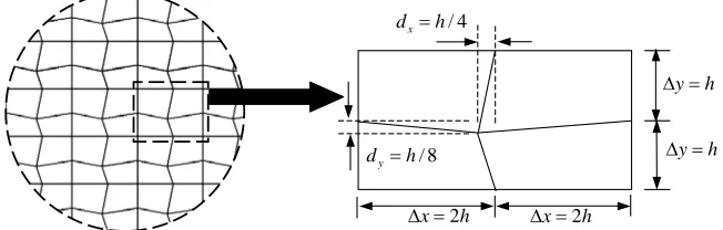
v u v u

D v u v u

x x y y

α α

− ₌ ⎡ ⎛∂ ∂ ⎞ ₊ ⎛∂ ∂ ⎞ _{+ ∇∇} ⎤

⎢ ⎜ _∂ _∂ ⎟ ⎜ _∂ _∂ ⎟ ⎥

⎢ ⎝ ⎠ ⎝ ⎠ ⎥

⎣ ⎦

∑

C∇∇ , (34)

where is the element index and e

( )

i i, _erepresents inner product taken over the interior of

element . It is important to note that the MAG coefficients for a given element are completely

determined using its geometry and material properties, and are independent of the other element

properties. Due to this local nature, the method is named local MAG (L-MAG) method. Such

(40)

dispersion error. The remainder of the paper focuses on the development and testing of the

L-MAG method for non-uniform rectangular meshes with bilinear elements.

Noting that, for bilinear rectangular meshes, the only nonzero second derivative is

2 h u x y

∂ ∂ ∂ , the L-MAG term simplifies to:

(

)

2 2

, , , ,

h h h h h h

L MAG h h e e e

h x y xy

e _e _e

v u v u v u

D v u

x x y y x y x y

α α β − ₌ ⎡ ⎛∂ ∂ ⎞ ₊ ⎛∂ ∂ ⎞ ₊ ⎛∂ ∂ ⎤ ⎢ ⎜ _∂ _∂ ⎟ ⎜ _∂ _∂ ⎟ ⎜_{∂ ∂ ∂ ∂} ⎥ ⎢ ⎝ ⎠ ⎝ ⎠ ⎝ ⎥ ⎣ ⎦

∑

e ⎞ ⎟

⎠ . (35)

The L-MAG coefficients ( e x

α , e

y

α and e xy

β ) of an element can be chosen such that the

dispersion error is minimized when the element is used in a uniform mesh. While not losing any

generality, such a treatment greatly simplifies the derivation and the results from section 3 can be

utilized. For uniform rectangular meshes with element size of ∆ × ∆x y, the terms for the coefficient matrix (11) for the L-MAG method is given by (see section 3 for details):

2 2 2

0

2 2 2

,

3 9 3 3

2

,

6 18 3 6

2

,

6 18 6 3

.

6 36 6 6

y xy x y x x x y x x y y x x xy x y

x y k x y

S

y

x y x y

x y

x y k x y

S

x y

x y x y

x y

y x k x y

S

x y

x y x y

x y

x y k x y

S

x y

x y x y x y

α β α α β α α β α α β α ∆ ∆ ∆ + ∆ ∆ ∆ = − + + + ∆ ∆ ∆ ∆ ∆ ∆ ∆ ∆ ∆ − ∆ ∆ ∆ = − − + − ∆ ∆ ∆ ∆ ∆ ∆ ∆ ∆ ∆ − ∆ ∆ ∆ = − + − − ∆ ∆ ∆ ∆ ∆ ∆ ∆ ∆ ∆ + ∆ ∆ ∆ = − − − − + ∆ ∆ ∆ ∆ ∆ ∆ (36)

Substituting the above in the dispersion relation (18) results in the dispersion relation

specific to L-MAG method:

(

)(

2 2

)

(

2 2

)

(

2 2

) (

)

2 2

12 6 6 2 6 2 4 2 2

6 2 2 6 2 2 36 1 0

x y x y x y x y

y x y x y x y x x y xy x y x y

C C x y C x y C y x C C C C x y k

xα C C C C yα C C C C β C C C C

− ∆ + ∆ + ∆ − ∆ + ∆ − ∆ − + + + ∆ ∆

⎡ ⎤ ⎡ ⎤ ⎡

+ ∆ _⎣ + − − _⎦+ ∆ _⎣ + − − _⎦+ _⎣ − − + =

(41)

where Cx and Cy are given in (17). In the preliminary version of this method [20],

e x

α is

chosen such that the dispersion error is eliminated ( ) for wave propagating along the

x-axis ( ). Substituting and in (37) results in:

h k k = 0 = θ h

k =k θ =0

(

)

(

)

2 2 2 cos

1

1 cos 6

e x

k x k x k x

α = + ∆ ∆ −

− ∆ . (38)

Similarly, e y

α is evaluated by eliminating the dispersion error in direction by letting

and :

y θ =90

h k =k

(

)

(

)

2 2 2 cos

1

1 cos 6

e y

k y k y k y

α = + ∆ ∆ −

− ∆ . (39)

From (37), (38) and (39), it can observed that there is no choice of βxy(independent of θ) that

would completely eliminate the dispersion error. Instead, one can significantly reduce the

dispersion error by choosing:

2 2

2 2 2

2 y x xy

x y

x y k

α α

β = −⎛_⎜ + ⎞ ∆ + ∆_⎟

∆ ∆

⎝ ⎠ . (40)

The L-MAG coefficients in (38), (39) and (40) represent the original variant of the L-MAG

method. This ad-hoc choice of L-MAG coefficients can be significantly improved by systematic

procedure followed in the next section.

2.6 Systematic Design of L-MAG methods

In this section, the dispersion relation for the L-MAG methods (Equation (37)) is

systematically utilized to obtain a set of dispersion reducing methods with increasing accuracy

(42)

parameters α α βx, y, xy can be chosen independently). With the expectation of significantly

reducing dispersion in all the directions, we chose to eliminate dispersion errors along the mesh

lines (θ1 =0, 90θ2 = ), and along the direction perpendicular to the main diagonal

(

1

3 tan x/ y

)

θ ₌ − _{−∆ ∆} _{. Three distinct equations are obtained by substituting}

1, 2, 3

θ θ θ θ= ,

each of them is linear in α α β_x, _y, _xy. These equations can then be solved to obtain the expressions for α α βx, y, xy in terms of k,∆ ∆x, y. As one would expect, the results for α αx, y

are given by (38) and (39). However, the expression for βxy takes a rather complex form that

would involve tricky computations. In order to simplify the computation for βxy, the

polynomial approximation based on Taylor’s expansion around k x∆ = ∆ =k y 0 is employed. For consistency purposes, αx and αy are approximated in a similar way. Such approximations

lead to a series of MAG methods. These methods are named as MAG2, MAG4, and

L-MAG6 reflecting the order of approximation (2, 4 or 6) used in Taylor’s expansion.

The parameters α α β_x, _y, _xy as well as the associated dispersion errors for various L-MAG methods are shown in Table 2-1 (for lumped integration of mass matrix) and Table 2-2 (for

consistent integration). The tables also include parameters for GLSm and “Residual” methods,

since each of these methods can be represented using equivalent L-MAG methods with identical

dispersion properties.

From the dispersion errors for various methods presented in Tables 2-1 and 2-2, we can

(43)

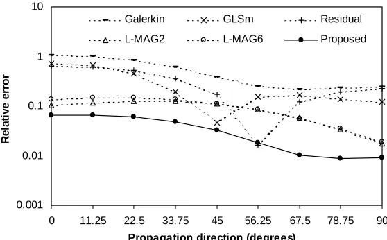
(a) For square meshes, all the L-MAG methods are superior to GLSm method. The

best available L-MAG method (L-MAG6) has almost identical error properties as the

best available dispersion reducing method (Residual method/GFEM).

(b) For rectangular meshes, the errors for all the L-MAG methods are considerably less

than any of the existing dispersion reducing methods.

(c) The second order method (L-MAG2) is a very simple modification of the Galerkin

method, and, although not as good as L-MAG6, is effective in reducing the

dispersion error for both rectangular and square meshes.

It thus appears that L-MAG framework resulted in a spectrum of dispersion reducing schemes

ranging from simple methods (L-MAG2) to highly accurate methods (L-MAG6).

2.7 Implementation of L-MAG Finite Element Methods

L-MAG FEM essentially differs from standard Galerkin FEM in that the coefficient matrix

in (9) is augmented with additional coefficient matrix arising from the MAG term:

, (41)

L MAG Gal L MAG

Aug

− ₌ ₊

S S S −

where L MAG is the coefficient matrix arising from the MAG term and is given by:

Aug

−

S

L MAG

Aug x y xy

− ₌ ₊ ₊

S S S S , (42)

where,

2 2

, ,

x x

y y

x x

y y

α

β

∂ ∂

⎛ ⎞

= _⎜ _⎟

∂ ∂

⎝ ⎠

⎛∂ ∂ ⎞

= _⎜ _⎟

∂ ∂

⎝ ⎠

⎛ ∂ ∂ ⎞

=

N N S

N N

S

Novel Finite Element Methods for Wave Propagation Modeling

ABSTRACT

Novel Finite Element Methods for Wave Propagation Modeling

by

Bin Yue

A dissertation submitted to the Graduate Faculty of

North Carolina State University

in partial fulfillment of the

requirements for the Degree of

Doctor of Philosophy

Civil Engineering

Raleigh

2004

APPROVED BY:

_________________________

Murthy N. Guddati

(Chair of Advisory Committee)

__________________________ _________________________

Vernon C. Matzen

M. Shamimur Rahman

__________________________ _________________________

BIOGRAPHY

ACKNOWLEDGEMENTS

Table of Contents

List of Tables

List of Figures

1 Introduction

1.1 Numerical Modeling of Wave Propagation

1.2 Preliminaries

( )

[ ]

(

)

(

)

(

)

(

)

(

)

(

)

( )

( )

( )

( )

(

)

(

)

(

)

(

)

( )

( )

( )

( )

(

)

(

)

1.3 Background and Objectives

1.4 Organization

References

2 Local Mesh-dependent

Augmented Galerkin Methods for

Reducing Dispersion Error for Helmholtz Equation

2.1 Introduction

2.2 Finite Element Method for Time-Harmonic Wave Propagation

Problems

( )

(

)

(

)

( ) (

)

(

__ _

__ _

_∫