Unified Framework to Evaluate Panmixia and Migration Direction Among Multiple Sampling Locations

(1)

DOI: 10.1534/genetics.109.112532

Unified Framework to Evaluate Panmixia and Migration Direction

Among Multiple Sampling Locations

Peter Beerli

1

_{and Michal Palczewski}

Department of Scientific Computing, Florida State University, Tallahassee, Florida 32306

Manuscript received November 27, 2009 Accepted for publication February 17, 2010

ABSTRACT

For many biological investigations, groups of individuals are genetically sampled from several geographic locations. These sampling locations often do not reflect the genetic population structure. We describe a framework using marginal likelihoods to compare and order structured population models, such as testing whether the sampling locations belong to the same randomly mating population or comparing unidirectional and multidirectional gene flow models. In the context of inferences employing Markov chain Monte Carlo methods, the accuracy of the marginal likelihoods depends heavily on the approximation method used to calculate the marginal likelihood. Two methods, modified thermodynamic integration and a stabilized harmonic mean estimator, are compared. With finite Markov chain Monte Carlo run lengths, the harmonic mean estimator may not be consistent. Thermodynamic integration, in contrast, delivers considerably better estimates of the marginal likelihood. The choice of prior distributions does not influence the order and choice of the better models when the marginal likelihood is estimated using thermodynamic integration, whereas with the harmonic mean estimator the influence of the prior is pronounced and the order of the models changes. The approximation of marginal likelihood using thermodynamic integration in MIGRATE allows the evaluation of complex population genetic models, not only of whether sampling locations belong to a single panmictic population, but also of competing complex structured population models.

I

NVESTIGATIONS using genetic samples from indi-viduals taken across a geographic or biological range— for example, water frogs caught at several ponds, blood samples of humans collected in several villages, or viruses collected from different host species that have the same disease—are common. Whether the individ-uals studied belong to a single population that is long-term randomly mating or to two or more populations that have varying degrees of genetic isolation from each other is an important concern. Because the geographic information about the locations often does not give a clear indication about the degree of genetic isolation of the individuals, we often use the genetic data them-selves to calculate test statistics to suggest whether or not the locations belong to the same population. Many programs (Hudsonet al.1992b; Michalakisand Excoffier 1996; Rousset 1996; Neigel 2002; Weir and Hill2002; Holsinger et al. 2002) use allele fre-quencies to calculateFST for pairs of locations or use Fisher’s exact test to reject panmixia for the whole or subsets of the data (Raymond and Rousset1995; Rousset2008).

Several methods test explicitly whether two popula-tions are or are not panmictic (for example, Hudson

et al. 1992a; Rousset1996). These methods are often applied to all pairs of a multiple-population data set. This is problematic, because both Beerli(2004) and Slatkin (2005) have shown that pairwise analyses can inflate the effective population size estimates, thereby confounding estimators of migration that use the effec-tive number of migrants.

Alternatives to tests based on allele frequencies have been implemented, for example, in the programs STRUCTURE (Pritchardet al.2000), BAPS (Corander

et al.2008), and STRUCTURAMA (Huelsenbeckand Andolfatto 2007). These methods allow the assign-ment of individuals to groups using the compatibility of their multilocus genotypes. They can thus be used to group locations into panmictic units on the basis of allele profiles and geography; this capability led to many advancements in landscape genetics and phylogeogra-phy. If we are interested in directionality of migration, however, this framework is often insufficient because the assignment methods offer only limited insight into population processes, such as migration, mutation, or fluctuation of population size, that underlie and ac-count for the present genetic structure (Palsbøllet al. 2007).

We describe here another alternative, using Bayesian inference, that calculates probabilities of explicit pop-ulation models using coalescence theory (a historical Supporting information is available online athttp://www.genetics.org/

cgi/content/full/genetics.109.112532/DC1.

1_{Corresponding author:} _{Department of Scientific Computing, Dirac} Science Library 150-T, Mailbox 4120, Florida State University, Tallahassee, FL 32306-4120. E-mail: [email protected]

(2)

review is given by Kingman2000). An extension of the original n-coalescent of Kingman to multiple popula-tions with migration (Strobeck1987; Hudson1991) leads to probabilistic inference programs that consider potentially complex migration patterns among sam-pling locations (for example, Beerliand Felsenstein 2001; Beerli2006; Kuhner2006). The program MIGRATE (Beerliand Felsenstein2001; Beerli2006) allows the calculation of a likelihood ratio test (LRT) for nested population models, but these calculations only approx-imate the LRT (Beerli2008), need a moderately com-plicated approach with several independent runs (Beerli 2009), or require time-consuming large-scale simulations (Carstenset al.2005). In our approach, a Bayes factor (BF) takes the role of an LRT. BFs and LRTs are not equivalent, however: the BF is the ratio of the marginal likelihoods of two hypothesesM1andM2, whereas the LRT measures support for one hypothesis over another at the maximum likelihood. BFs are better suited for model selection than LRTs because one can compare nonnested as well as nested models. In addition, the programm-ing and the successful application of Bayesian inference programs are often simpler than maximum likelihood (Beerli2006).

Here, we report on the effect of two different ap-proximations of the marginal likelihood on BF and therefore on the support for specific population mod-els. We provide examples of the use of these methods to extend our tool set for investigating whether sampling locations are part of a panmictic population or are parts of a more complex population structure. Our approach unifies the analysis of population models and allows a wide spectrum of comparisons, from simple tests of whether locations sampled are part of a single popula-tion to more complex quespopula-tions, such as whether there are unambiguous migration directions among popula-tions; it also calculates posterior distributions of param-eters of these models.

MATERIALS AND METHODS

Our approach to population model selection uses a frame-work that allows inferring parameters using coalescence theory. The population models are simple structured coales-cence models with possibly many parameters (Beerli and Felsenstein2001).

Bayes Factor estimation: In a typical Bayesian inference using Markov chain Monte Carlo (MCMC) methods we do not need to calculate the marginal likelihood to estimate the pos-terior probability distribution of the parameters of a specific model because the MCMC analysis depends only on likelihood ratios and not absolute likelihoods. Because BF is a ratio of marginal likelihoods of two models, however, calculation of these absolute likelihoods is essential. Because we use absolute likelihoods, we can now easily compare more than two models with the BF framework by choosing a reference model and comparing or ranking other candidate models with that.

We augmented the program MIGRATE (Beerli2006) with a module to calculate the marginal likelihood

LMi ¼PðDjMiÞ ¼

ð Ci

PðC_ijMiÞPðDjC_i;MiÞdC_i; ð1Þ which is the probability density of the data where the pa-rameters, for example population sizes and migration rates, and nuisance parameters, for example genealogiesCi, of the model Mi are integrated out using the prior distribution

PðCijMiÞ. The marginal likelihood is difficult to estimate with sufficient accuracy because not only the region around the mode, but also the tails of the distribution need to be ex-plored. This is not straightforward in an MCMC context where we bias toward more likely solutions and so have a tendency to sample the tails of the distribution less frequently. The marginal likelihood is calculated in a Bayesian context and needs proper prior distributions to exist. Improper priors would lead to infinitely large tails that do not allow a consistent estimate of the marginal likelihood. We contrast two different methods to estimate the marginal likelihood: harmonic mean (Newtonand Raftery1994; Kassand Raftery 1995) and path sampling (Gelman _{and M}eng _{1998). Studies of path} sampling have recently led to an alternative method of esti-mating marginal likelihoods (thermodynamic integration) (Gelman and Meng 1998; Lartillot and Philippe 2006; Frieland Pettitt2005, 2008).

Harmonic mean estimator: Newtonand Raftery(1994) described an approximation of Equation 1 using a harmonic mean estimator. Our stabilized harmonic mean estimator is a natural adaptation of Newton and Raftery’s harmonic mean estimator to problems that treat genealogies as nuisance parameters and summarize over all possible genealogies G

using the Metropolis–Hastings algorithm (our MCMC sampler was described in detail by Beerli 1998, 2006 and Beerli and Felsenstein1999, 2001). We approximate the marginal likelihood as

LHM¼PðDjMiÞ 1

m

Xm j¼1

1

PðDjGjÞ

!1

: ð2Þ

The extension from single-locus to multilocus data is not straightforward even with unlinked loci. We developed a method for combining independently inferred marginal like-lihoods that allows fast parallel computation of unlinked loci. The combined marginal likelihoods are the product of the independent marginal likelihoods for each locus and a scaling factorKfor loci,

LHMðallÞ¼K

YZ z¼1

PðDzjMiÞ: ð3Þ The scaling factor

K ¼

ð

P

YZ z

PðDzj P;MiÞPðP jMiÞ1Z_d_P_; _ð₄_Þ

whereZis the number of loci. We describe the scaling factorK

in detail in theappendix.Kcan be approximated using prior, likelihood, and posterior values reported during the MCMC run (appendix). Our program MIGRATE version 3.1 calcu-lates K and reports locus-specific and combined marginal-likelihood values when multiple loci are used.

(3)

allows exploring these low-likelihood areas by distorting the acceptance ratio of the MCMC procedure with scaling factor tranging from zero to 1.0, where att¼0.0 the process samples from the prior distribution and att¼1.0 it samples from the distribution of interest. Thus, we calculate the log marginal likelihood using the expectation of the distribution of all coalescent genealogiesGgiven the dataDevaluated at scaling factort,

‘TI¼lnPðDjMiÞ ¼

ð1 0

E_G_jD_;_t_ln_PðDjG;MiÞdt: ð5Þ We approximate this integral using the trapezoidal rule for the scaling factort, using a small number of scaling valuest0¼0, t₁,. . .,tk,. . .,tn¼1 and the corresponding marginal likelihoodsy0. . .ynas

‘TI¼

Xn k¼2

ðtktk1Þ

yk1yk1

2 ð6Þ

with the average of log likelihoods, ln P(DjGj,Mi), at a given scaling valuetk,

yz¼ 1 m

Xm j¼1

lnPtkðDjGj;MiÞ: ð7Þ For multiple unlinked loci we then use

‘ð_TIallÞ¼lnKX Z

z¼1 ‘z

TI: ð8Þ

TheKis the same as the one in Equation 4. MIGRATE already used a scheme to run parallel MCMC chains to improve the exploration of search space using discrete scaling values tk that is based on the scheme proposed by Geyer and Thompson(1995): Metropolis coupled Markov chain Monte Carlo (MCMCMC). They formulated their method in terms of thermodynamic properties in which a chain that accepts always, witht¼0.0, is the hottest chain with a temperature of 1/t ¼ ‘ because the chain bounces randomly in many different areas of the search space, and a chain witht¼1.0 is cold because its movements are smaller. After each chain attempts a change of the genealogy, the system allows for swapping trees among neighboring MCMC chains with scaling factorstiandti11 to improve the parameter estimates. The

swap ratio depends on the relative likelihood ratios of ran-domly chosen pairs of chains with differenttand is

r,PðDjGiÞ

ti1_P_ð_D_j_Gi 1Þti

PðDjGiÞti_P_ð_D_j_Gi_1Þti1; 1,i,n; ð9Þ whereris a uniform random number between 0 and 1, andnis the number of chains with different scaling factorst. We use the term scaling classes to express the different discrete classes with different values oft. One could express the same classes as temperature classes where the temperatureTiis 1/ti.

For the thermodynamic integration we record the likeli-hood values for each chain; these values are then used to cal-culate the averagesyk, which are used to calculate the marginal likelihoods. This is a static variant of the step-stone method proposed by Wangang Xie, Ming-Hiu Chen, Yu Fan, Lynn Kuo, and Paul Lewis (L. Kuoand P. Lewis, personal communica-tion in 2008).

Using discrete classestkmay be too simple for phylogenetic applications (cf.Lartillotand Philippe2006), but results in consistent estimates even for few scaling classes (Figure 1), except that the magnitudes of the estimates of the marginal likelihood (the area under the curve) are correlated with the

number of scaling classes. The calculation time for each scaling class is about the same, so a run with 4 scaling classes will be about eight times faster than a run with 32 scaling classes. In principle, the different chains can be run in parallel, but the gain in speed is limited because the chains run in lockstep and need to wait on the slowest chain. Because many simulations (not shown) revealed that the shape of the path sampling function (Figure 1) is very similar with different migration models, we propose a different treatment of the first (the hottest) interval, defined by the scaling factorst₀andt₁ with log-likelihood valuesy0andy1, respectively. We calculate

the area of this first interval analytically, using a cubic Be´zier spline with two additional control pointsc(0)_and_c(1)_{that are}

calculated using the first three points. A point is a pair oftiand log-likelihoodyiand is defined aspi¼(ti,yi). The additional control points are

cð0Þ_¼ _t 0;

1 5y01

4 5y1

ð10Þ

cð1Þ¼ t0;

t1y2t2y1

t1t2

ð11Þ

so that we have four control points

pt;y¼ ððt0;y0Þ;cð0Þ;cð1Þ;ðt1;y1ÞÞ: ð12Þ The values of they-axis of the additional control points were chosen so that the Be´zier curve mimics the path sampling function estimated with many scaling classes. We calculate a pointp(w)_{on the Be´zier function using}

ptðwÞ;yðtÞ ¼

X3 i¼0 3 i

pðiÞt;yt ið1tÞ31

: ð13Þ

The partial marginal likelihood by integrating the parametric function over the hottest interval is then

‘ðt0;t1Þ¼

ð1 0

pyðwÞðtÞ dpðwÞt

dt dt ð14Þ

¼ 1

20ððt1t0Þðy013c

ð0Þ y 16c

ð1Þ

(4)

the estimation of large problems with many parameters can take a long time to run.

Simulation studies to test the approximations to the mar-ginal likelihood:The quality of the two estimators‘^TIand‘^HM

was tested using simulated data. These data sets were gener-ated using a coalescence-based simulator (distributed from

http://people.sc.fsu.edu/beerli/programs).

One- and two-population simulations:The HM and TI approx-imations were compared with a standard test statistic based on allele frequencies (Hudsonet al.1992a), using two groups of simulated two-population data:

1. One hundred artificial DNA data sets containing 1000 sites for 10 individuals in each of two populations using a model with no immigration into population 2 with parameters Q₁ ¼ 0.005, Q₂ ¼ 0.01, M2/1¼100, M1/2¼0 were

analyzed with nine different models.Qis the mutation-scaled effective population size, 4Nem, andMis the ratio of

the immigration ratemand the mutation ratemper site and generation. The marginal likelihoods of eight alterna-tive models were then compared with the marginal likeli-hood of the model used to simulate the data, the ‘‘true’’ model. This comparison of marginal likelihood ratios is equivalent to Bayes factors.

2. Simulations of four sets of 100 single-locus data sets with different degrees of isolation from each other were used to compare the Bayes factor method against a traditional test based on frequencies. These four sets were simu-lated with (a)Q¼0.01 and the 20 individuals randomly split into two groups; (b) Q1 ¼ Q2 ¼ 0.005, M2/1¼

M1/2¼500;000 (this is equivalent to a totalNm¼1250);

(c)Q₁¼Q₂¼0.005,M2/1¼M1/2¼100 (this is equivalent

to a totalNm¼ 0.25); and (d)Q1¼Q2¼0:005;M2/1¼

M1/2¼1 (this is equivalent to a totalNm¼0.0025). The

analyses of these four sets were done for two models, a single-population model and a full two-single-population model.

Large-scale population simulations: Many real problems in-clude many sampling locations for which the association of sampling locations and panmictic populations is unknown. We simulated data for 50 loci from 3 populations using a scenario as outlined in Figure 2A. This stepping-stone model has five parameters and for each locus 300 bp were simulated using these values:Q1¼0.003,Q2¼0.003,Q3¼0.004,M1/2¼100,

M2/3¼100. The individuals (120, 120, and 160) in the 3

populations were then randomly grouped into 6, 6, and 8 sampling locations, respectively. The full data set contained 20 locations with 20 individuals each. These particular settings were chosen because they mimic potential data sets that use anonymous loci from the nuclear genome. A naive application

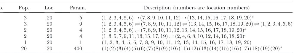
of these data would ask for a 20-population analysis. With a default MIGRATE run we would need to estimate 20 popula-tion sizes and 380 migrapopula-tion parameters, a daunting task with few loci. A total of six potential migration models using dif-ferent numbers of populations and difdif-ferent migration models were explored. The six cases presented use models with 1, 2, 3, and 20 populations with several candidate models (Table 1, Figure 2). Specific MIGRATE run conditions are described in supporting information,File S1.

TABLE 1

List of migration models used for simulation study

No. Pop. Loc. Param. Description (numbers are location numbers)

1 3 20 5 ð1;2;3;4;5;6Þ/ð7;8;9;10;11;12Þ/ð13;14;15;16;17;18;19;20Þa

2 3 20 9 ð1;2;3;4;5;6Þ_ð₇;8;9;10;11;12Þ_ð₁₃;14;15;16;17;18;19;20Þ_ð₁;2;3;4;5;6Þ 3 2 20 4 ð1;2;3;4;5;6Þ_ð₇_;₈_;₉_;₁₀_;₁₁_;₁₂_;₁₃_;₁₄_;₁₅_;₁₆_;₁₇_;₁₈_;₁₉_;₂₀_Þb

4 2 20 4 ð1;3;5;7;9;11;13;15;17;19Þ_ð₂_;₄_;₆_;₈_;₁₀_;₁₂_;₁₄_;₁₆_;₁₈_;₂₀_Þc 5 1 20 1 (1, 2, 3, 4, 5, 6, 7, 8, 9, 10, 11, 12, 13, 14, 15, 16, 17, 18, 19, 20)

6 20 20 400 (1)(2)(3)(4)(5)(6)(7)(8)(9)(10)(11)(12)(13)(14)(15)(16)(17)(18)(19)(20)d

No., model number; Pop., population; Loc., location; Param., parameter. a

See Figure 2A (true model). b

See Figure 2B. c

See Figure 2C. d

Each location is connected with all others; see Figure 2D.

(5)

Effect of prior choice and prior range: We explored the effect of the choice of the prior distribution on the marginal likelihood by using simulated multilocation single-locus data. We compared two exponential and two uniform prior distri-butions: narrow uniform prior distribution forQandMwith a minimum of 0.00001, 0.0 and a maximum of 0.1, 5000, respectively; a wide uniform distribution with a maximum for QandMof 0.5 and 50,000; a narrow exponential distribution with the same minimum and maximum as the narrow uniform but a mean of 0.01 and 100 forQand M, respectively; and a wide exponential distribution with minimum and maxi-mum of the wide uniform, but with a mean of 0.1 and 1000, respectively. Specific MIGRATE run conditions are described inFile S1.

Model selection: Model choice probabilitiessiwere calcu-lated as suggested by Kassand Raftery(1995) by

si¼PBFn i j BFj

: ð16Þ

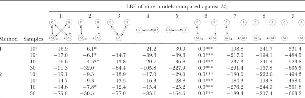
Example data set:Our example problem reanalyzes part of a data set of humpback whales from four sampling locations in the Southern Atlantic collected by Engel et al. (2008): near Brazil, Antarctica 1 (west of the Antarctic peninsula), Antarctica 2 (east of the Antarctic peninsula), and Colombia (Figure 1 in Engel et al. 2008). The data were analyzed using several different migration models. We used three subsamples of the original data, two with 10 and one with 30 randomly selected individuals from each location. We also ran one of the data sets twice for all example models to assess the effect of the Markov chain Monte Carlo error. We established a most likely mutation model within the constraints for MIGRATE by using PAUP* (Swofford2003) to estimate parameters for site rate variation and transition/transversion ratio.

RESULTS

Comparison of approximations of the marginal likelihood: In all but trivial situations we cannot cal-culateLMor its log value,lM, analytically. Using simu-lated data, we compared the two different methods for approximating LM: the thermodynamically estimated

^

‘ðTIiÞ_{using coupled scaling classes TIi}_{and the harmonic}

mean HM estimated as ‘^ðHMÞ_{. In the context of} co-alescent simulations the artificial dataDisimulated from a set of true parameter values still include considerable variability, so we do not expect a particular‘^M(for short:

^

‘) from all data sets. Nevertheless, we expect that the different approximations will result in the same‘^for a specific data set. Figure 3 shows a comparison of the two different approximations oflM. The relative magnitude of‘^among the different data sets is the same: a data set that shows low‘^with the HM estimator also shows low values for the different TI schemes.‘^ðHMÞ_{is little affected} by the number of scaling classes, whereas the number of scaling classes affects the absolute value of the‘^ðTIÞ_. When the results of a specific data set are compared, the TI4method delivers lower‘^than the HM4, HM16, HM32, TI16, and TI32 methods. The thermodynamically esti-mated‘^ðTIcÞ_{using independent scaling classes is}

identi-cal to the coupled sidenti-caling classes (data not shown).

Bayes factor estimation: Instead of reporting BF, we report its log-equivalent LBF, which is lnðLM2=LM1Þor

ð‘M2‘M1Þ. The log marginal-likelihood values

^

‘ are dependent on the approximation, and the LBF de-pends on the difference of the log marginal likelihoods

^

‘and therefore the relative difference among models is more important than the unbiased recovery of‘^(Figure 3). Figure 4 compares the dependency of the approx-imations on the length of the run. The shortest run took only 5 sec with four chains, visiting 30,000 states and discarding the first 10,000; the longest four-chain run took 5 min 21 sec, visiting and discarding 256 times more states. The thermodynamic integration approxi-mation results in LBFs with high repeatability and little variance even with only short runs, whereas the LBFs using the HM estimator are unstable even for long runs, and it appears that MCMCMC searches with many chains result in reduced reliability of the HM estimators.

Numerous artificial single-locus data sets from a model with two populations of unequal size, in which only one population receives migrants from the other, were generated; this model has three parameters that are free to vary: population sizes 1 and 2 and immigration rate from population 2 to population 1, which isM0¼ h)

_n

. Populations are indicated by squares. Two open squares indicate populations constrained to have the same size; one open and one solid square indicate population sizes are not constrained. Arrows indicate allowed migration direction [from population 1 to 2, from 2 to 1, or in both directions; arrows with two heads indicate symmetric migration rate parameters (M¼m/ m)]. These data sets were analyzed with all nine possible simple models (one parameter, h_{; two parameters,} h4

_n

, h/

_n

, h)h_{; three parameters,} h/

_n

, h)

_n

,h4

_n

,h !h; four parameters,h !n); models that exclude gene flow among the populations were

Figure 3.—Comparison of the log marginal likelihood

(6)

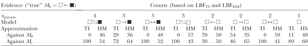
omitted. We calculated log Bayes factors, LBF¼ ð‘^_M_i‘^_M₀Þ. These report the chance of accepting Mi overM0. In Table 2 LBF using TI16rejects models that have more parameters than the true model or that disregard unidirectional migration with high frequency. Very simple models and asymmetric models are often accepted as plausible models. LBF using HM is in-decisive, even with models that are very different from the true model, such ash4h_{. Overall, the estimates} from TI deliver a clearer guide about which models to prefer than the highly variable HM estimates (seeFile S1), which, on average, are less decisive.

A comparison with different strengths of migra-tion rate among two populamigra-tions (Table 3) shows that the LBFTI4 is more variable than the LBFTI16 but the numbers of acceptances or rejections of a hypothesis (Table 3, Table 2S inFile S1) are very similar between TI16and TI4. In contrast, the LBFHMhas a higher vari-ability of outcomes.

Comparison with a panmixia test method:Currently, coalescence-based inference programs do not test whether the sampling locations are in separate popu-lations or not. Therefore, summary statistics such as

FST, Fisher’s exact test, or population genetic clustering programs (Pritchard et al. 2000; Evanno et al.2005; Huelsenbeck and Andolfatto 2007; Manel et al.

2007; Guillot2008) are being used to establish groups of individuals or sampling locations that most likely form panmictic populations. Waples and Gaggiotti (2006) showed that contingency table permutation methods work well. Hudson, Boos, and Kaplan (Hudson

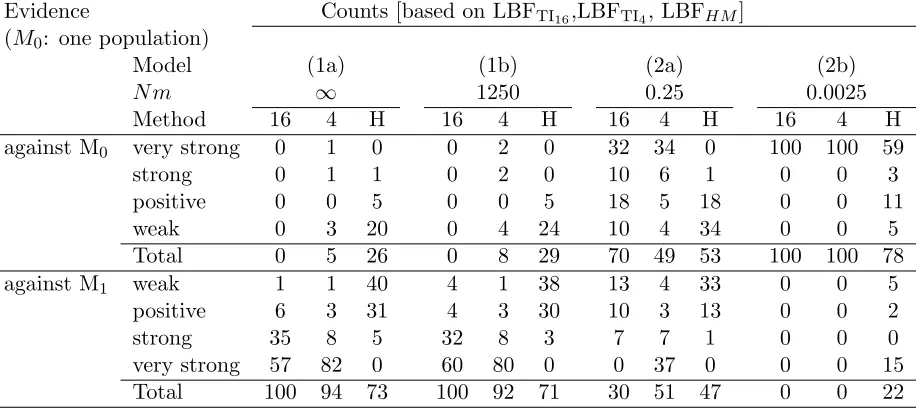
et al.1992a) developed a permutation test (HBK) that has great potential but seems to be little used despite its power to establish panmixia. For our comparison we used four scenarios: (1a) a single population was sam-pled and then the sample was randomly partitioned into two ‘‘populations’’, (1b) two populations exchanging 1250 migrants per generation, (2a) two populations exchanging 1 migrant every 4 generations, and (2b) two populations exchanging 1 migrant every 400 generations. Table 3 reveals that for a real panmictic population (1a), LBFTI16, LBFTI4, and LBFHMdetect panmixia in 100, 94, and 73 of the data sets, respectively, whereas HBK finds that all 100 data sets are panmictic. Recognition of panmixia in scenario 1b was 100, 92, and 71 for LBFTI16, LBFTI4, and LBFHM, respectively, whereas the HBK method marks all data sets panmictic. With LBFTI, all data sets from scenario 2b fit a two-population model; with 2a the acceptance of a two-population model shrank to 70, 49, and 53 of 100, signaling considerable uncertainty about finding the correct population model. HBK declares all data sets under scenario 2 to contain

Figure 4.—Comparison of

the LBF (ln BF) values for dif-ferent run lengths of the MCMC chain. The squares and circles are LBF values using the aver-age marginal likelihoods from five replicated runs. The verti-cal bars mark the range be-tween the largest and the smallest LBF value from five replicated runs. (A) LBF ap-proximated using the harmonic mean; (B) LBF approximated by thermodynamic integration. The simulated data were generated using modelM¼h)

_n

and LBF ¼ ð‘h/n‘h)nÞ. LBF scales in A and B are very different.

TABLE 2

Summary of support for specific models using LBF approximated with harmonic mean (HM) and thermodynamic integration (TI) using 16 chains with different scalers

Evidence (‘‘true’’M0¼h)

n

) Counts (based on LBFTIand LBFHM)

nparam 4 3 3 3 2 2 2 1

Model h_!n h/

_n

h4

_n

h_!h h)h h/h h4h h

Approximation TI HM TI HM TI HM TI HM TI HM TI HM TI HM TI HM

AgainstM0 0 46 28 36 0 48 0 57 70 50 54 35 0 59 11 40

AgainstMi 100 54 72 64 100 52 100 43 30 50 46 65 100 41 89 60

(7)

two populations. LBFHMshows, for all scenarios, much larger variability in acceptance and rejection of pan-mixia (seeFile S1), resulting in a lower total acceptance of the correct model.

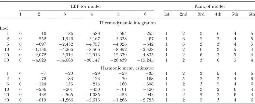
Effect of loci and model complexity: Table 4 shows the LBFs for six migration models (Table 1). The ther-modynamic integration method consistently chooses the true model as the best model. Differences for the other models depend on the haphazard choice of the order of the loci. Because only 50 loci were simulated for all runs, the first locus is shared among all runs, and the second locus is shared among all runs except the 1-locus runs, etc. We expect that with many loci a clear order of models is achieved. The model order for the 50-locus run is 1, 2, 3, 6, 5, and 4. Runs with many loci (.10) suggest that the one-population model (5) is superior to

the two-population model that combines the locations in an intermixed pattern (4) and also suggest that the 400-parameter (6) analysis is preferable over analyses with wrongly combined locations. Runs with only few loci may suffer because there are not enough data to correctly rank incorrect models 3, 4, 5, and 6. The reported Bayes factor values suggest that model 1 should be picked with probability 1.0 over the five alternatives. More loci increase this certainty consider-ably: the difference between the first and the second best model is already very large for a single locus. The number of loci and the BF differences are positively correlated. The results for the harmonic mean estima-tor suggest that the preferred model is the 9-parameter model (2) and not the model that was used to simulate the data (1).

TABLE 3

Comparison of the influence of the approximation on the power of LBF for simple models with different migration schemes

Evidence Counts (based on LBFTI16, LBFTI4, and LBFHM)

Model 1a 1b 2a 2b

Nm ‘ 1250 0.25 0.0025

Approximation 16 4 H 16 4 H 16 4 H 16 4 H

AgainstM0 0 5 26 0 8 29 70 49 53 100 100 78

AgainstM1 100 94 73 100 92 71 30 51 47 0 0 22

LBF compared a full model (modelM1¼h!n) with a panmictic population (modelM0¼h). Models used to simulate the

data were as follows: 1a, a single population, the sampled individuals split randomly into two sets (Nm/‘); 1b, two populations exchanging many migrants (Nm¼1250); 2a, two populations exchanging a moderate number of migrants (Nm¼0.25); and 2b, two populations with very low migration rate (Nm¼0.0025). The marginal likelihoods used in the LBF were approximated with thermodynamic integration (TI) with 16 and 4 scaler bins and with the harmonic mean (HM4).

TABLE 4

Comparison of log Bayes factors (marginal log-likelihood differences) approximated by thermodynamic integration and harmonic mean estimator, for different models and different numbers of loci

LBF for modela _{Rank of model}

1 2 3 4 5 6 1st 2nd 3rd 4th 5th 6th

Thermodynamic integration Loci

1 0 10 86 583 594 253 1 2 3 6 4 5

2 0 552 1,946 3,167 3,338 467 1 6 2 3 4 5

5 0 697 2,432 4,757 4,826 542 1 6 2 3 4 5

10 0 1,136 4,266 8,566 8,352 2,328 1 2 6 3 5 4

20 0 2,072 5,914 12,913 12,379 4,835 1 2 6 3 5 4

50 0 4,829 14,683 30,147 28,439 15,245 1 2 3 6 5 4

Harmonic mean estimator

1 0 7 20 29 28 35 1 2 3 5 4 6

2 0 76 83 123 70 168 1 5 2 3 4 6

5 0 124 133 215 160 308 1 2 3 5 4 6

10 0 236 201 430 161 420 1 5 3 2 6 4

20 0 438 565 1,085 453 943 1 2 5 3 6 4

50 0 819 1,266 2,613 1,266 2,723 1 2 5 3 4 6

(8)

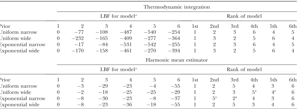
Effects of prior distribution on the marginal likeli-hood: Table 5 reveals that the marginal likelihoods depend on the prior distribution: the LBF values are different for different prior distributions. For the ther-modynamic integration method, however, the order of the models is identical among the narrow and wide prior distributions, respectively, suggesting that most likely the runs were rather short for the wide-prior models. The harmonic mean estimator of the marginal likelihood is similarly affected by the choice of prior distributions. Using the harmonic mean estimator, the models are ranked differently for each of the different priors.

Example analysis of migration patterns among humpback whales sampling locations in the south seas:

Olavarrı´a et al. (2007) and Engel et al. (2008) de-scribed the interaction of several humpback whale populations (sampling locations). We use parts of their data to showcase how BF can inform the discussion of whether whales from these sampling locations belong to the same genetic population or not and whether some population models provide more appropriate descriptions than others. Our analysis does not com-pletely resolve the complex population interactions of humpback whales, but it shows ways in which our method is more useful than current methods for model comparisons. Engelet al.(2008), using pairwise

FSTestimates, suggested that Antarctic locations A1 and A2 appear panmictic; they used additional sighting data to suggest that the individuals sampled near the Brazilian coast probably do not move to the presumed feeding grounds in the Antarctic but instead aggregate at some unknown location. We chose a subset of models to investigate (1) whether the regions Antarctica 1 and 2 belong to a single population and (2) whether the

Brazilian individuals and Antarctic individuals belong to the same population. Table 6 shows the ‘^for each model tested for three subsets of the full data set. Model 6, which allows for structure between A1 and A2 and reduced gene flow between Antarctica and Brazil, has the highest marginal likelihood. This model was used as the reference in LBF to compare all models. Our analysis confirms the conclusion of Engelet al.(2008) that the connectivity between the Brazilian and Antarctic locations is reduced (model 6), but, unlike models 7–9, does not suggest complete isolation of the Brazilian individuals from the other locations. Model 2 is the second best model; it shares almost all features of model 6 except that the migration rates between Antarctica and Brazil are bidirectional. Models that suggest A1 and A2 are part of a panmictic population (models 3–5) have lower LBF values than models 2 and 6, but model 3 is superior to model 1. This suggests that A1 and A2 are probably not part of a panmictic population, but the data do not support a complex model with many parameters (model 1). Our current understanding of the population structuring is based on a single locus (mtDNA). These data are insufficient to resolve the complex interactions among southern Atlantic hump-back whales.

The data sets were analyzed using TI with 32 chains and 4 chains. The Be´zier-corrected 4-chain marginal likelihoods result in LBF of the same magnitude as the 32-chain runs, despite the greatly reduced run time.

DISCUSSION

The approximation of lMusing the harmonic mean estimator is concordant with the thermodynamic

in-TABLE 5

Log Bayes factors (LBF) estimated by thermodynamic integration and by the harmonic mean using different prior distributions

Thermodynamic integration

Prior 1 2 3 4 5 6 1st 2nd 3rd 4th 5th 6th

Uniform narrow 0 77 108 487 540 254 1 2 3 6 4 5

Uniform wide 0 232 165 409 277 364 1 3 2 5 6 4

Exponential narrow 0 17 84 531 542 255 1 2 3 6 4 5

Exponential wide 0 170 158 461 270 394 1 3 2 5 6 4

Harmonic mean estimator

Prior 1 2 3 4 5 6 1st 2nd 3rd 4th 5th 6th

Uniform narrow 0 3 29 23 4 55 1 2 5 4 3 6

Uniform wide 0 2 18 25 25 29 1 2 3 5b ₄b ₆

Exponential narrow 0 8 30 23 8 37 1 5b ₂b ₄ ₃ ₆

Exponential wide 0 8 23 36 18 55 1 2 5 3 4 6

Model 1 was used to simulate the data and is also the reference model. a

(9)

tegration method, although the HM estimate is always higher than the TI estimator. Paul Lewis (P. Lewis, personal communication, 2009) has shown that this is an artifact of MCMC runs in which the HM estimator is biased toward the high probability regions of the parameter space. TI, in contrast, estimates very similar magnitudes of‘^over replicated runs of the same data and run parameters. Nevertheless, the magnitude of‘^ using the thermodynamic method is correlated with the number of classes, although the relative difference among models persists independently of the absolute magnitude. Using the Be´zier quadrature with a low number of chains at different scalers removes this dif-ference. The run time is dependent on the number of chains, so the use of the Be´zier quadrature may be preferable for large data sets and large population models because running many MCMC chains requires more time than is usually available in computer time budgets.

Analyses with different run lengths showed that the Bayes factor based on the harmonic mean estimator is more variable than that based on the thermodynamic integration estimator. Most disconcerting are the results with many chains because multiple LBF estimates based on the HM estimates show a wide range for the same data set, suggesting that an appropriate MCMC search results in unreliable HM estimates. The path of the MCMC chain influences the HM-based BF considerably because, for a good estimate of ‘, the chain needs to^ explore areas of the solution space that have low prob-ability. Once a low value is recorded, it affects the harmonic mean disproportionately. Runs that rarely visit such low values will report an ‘^that is inflated. Using such values in the LBFHMleads to high variance because the low values are not visited in the correct

proportions. Our results corroborate the work of other authors (for example, Lartillotand Philippe2006) who consider the HM inferior to the TI method.

The LBF usually supports the correct model inde-pendent of the number of chains used in the thermo-dynamic approximation method. In the comparison in Table 2, several models were weakly supported. This is interesting because these alternative models (h/

_n

,h)h;h/h_{), which are models with strong} unidirectional gene flow, are viable competitors for the real model (h)

_n

) given the small sample size (20 individuals) and the large variance in coalescent simu-lations. Without multiple loci it is particularly difficult to estimate the migration direction from genetic data that often differ only in the frequency of alleles. The multi-locus runs show the same general pattern as the analyses with few loci, but in the larger analyses the certainty of the order of models increases. The HM estimator is less certain for all scenarios than the TI estimator, corrob-orating the problems visible in Figure 4, suggesting again that the HM estimator should not be used.

LBF is relatively powerful for identifying appropriate models for samples from panmictic populations and well isolated populations, but showed a high variance for structured populations with moderate immigration rates (Table 3). In contrast, the Hudson–Boos–Kaplan estimator, using a permutation test, clearly suggested two populations for all analyzed data sets that were generated from models with reduced immigration rates. Because this test does not incorporate the un-certainty of the mutation model and the coalescence, however, it may overconfidently reject simpler (panmic-tic) interpretations.

It has been known for a while now through recent examples (Beerliand Felsenstein1999; Felsenstein

TABLE 6

Log Bayes factor (LBF) using thermodynamic integration of different gene flow modelsMicompared with model 6 for four sampling locations of humpback whales (C, Colombia; B, Brazil; A1, Antarctica east of the Antarctic

peninsula; A2, Antarctica west of the Antarctic peninsula)

LBF of nine models compared againstM6

Method Samples

1 2 3 4 5 6 7 8 9

1 10a _16.9 _6.1* _21.2 _39.9 _0.0*** _198.8 _241.7 _531.4

10a _17.0 _6.1* _14.7 _39.3 _39.3 _0.0*** _217.0 _194.1 _484.5

10 16.6 4.5** 13.8 20.7 36.8 0.0*** 237.3 241.9 523.8

30 91.3 32.0 84.4 105.8 227.9 0.0*** 291.4 167.8 605.5

2 10a _15.1 _9.5 _13.9 _17.0 _29.0 _0.0*** _180.0 _222.6 _494.3

10a _14.7 _9.3 _13.5 _16.3 _28.8 _0.0*** _184.3 _193.8 _458.0

10 14.6 7.8* 12.4 15.4 25.2 0.0*** 276.2 244.9 501.8

30 75.0 30.5 77.0 83.1 164.6 0.0*** 189.4 207.4 663.2

Method 1, using 4 chains and Be´zier approximation; method 2, using 32 chains. Model probabilities: *0.01,si,0.05; **0.05,

si,0.10; and ***0.9,si,1.0. a

(10)

2005; Heledand Drummond2008) that the number of unlinked loci increases the accuracy of the coalescent estimators considerably; our comparison of the effect of multiple loci is no exception. Rejection of incorrect models became stronger with more loci when the mar-ginal likelihood was approximated with thermodynamic integration. The harmonic mean estimator preferred a more complicated model with increased certainty, cor-roborating our findings with the two-population models (Tables 2 and 3) that the harmonic mean estimator should be avoided.

The Bayes factor framework demands proper priors, formally, priors that integrate to one. In our framework all priors are proper, although some may not be optimal: for example, uniform prior distributions over a very large range are wasteful because the posterior distribu-tion covers only a small range of values and forces very long runs for accurate estimates. Our experimentation with different prior distributions shows that suboptimal priors can often result in long run times before con-vergence. The effect on the marginal likelihoods, how-ever, seems small and the effect of such suboptimal priors on model choice seems negligible. In contrast, misspecification of the prior distribution, for example, choosing too narrow a prior distribution range, has a detrimental effect on the estimation of the posterior distribution of the parameters of the model and results in incorrect marginal likelihoods.

Our example (Table 6) confirms that, in a coalescence framework, a small sample per location has almost as much power as a large sample (cf.Felsenstein2005) because not only is the LBF of a replicated run the same with the same sample, but also different randomly sampled sets of the same and larger size return the same ranking among the models. The Be´zier-spline approx-imation of 4 chains gives LBF values that are equivalent to runs using 32 chains, but the run time is about one-eighth as long. This suggests that we are able to estimate LBF values of very large data sets in a reasonable time with good accuracy without the need to use a large number of chains or the reversible-jump MCMC (Green 1995) method that has recently been proposed by Lartillot (Lartillotand Philippe2006) in a phyloge-netic context. Our approach asks for independent runs for each model, in contrast to model selection approaches that use reversible-jump MCMC. This may look inelegant, but we believe that our method is pref-erable both because each run pays full attention to a single model and because the effort does not depend on the particular model-sampling algorithm and there-fore is independent of the geometry of the complex solution space. In any study, the number of models depends on the number of populations and increases at a superexponential rate, so it is unlikely to evaluate all possible models, in contrast to mutation models, all of which are able to be evaluated (Huelsenbeck and Ronquist2005). In addition, our scheme can be

run in parallel without problems and without further programming.

The simulation study clearly shows that BFs are capable of distinguishing between different models and allow us to retrieve the model that was used to simulate the test data with high certainty when the true parameters produced a clear scenario. Single-locus data will often not be sufficient to retrieve a fairly complex model unambiguously, so that when available data are few, we should prefer simple models. Of course, multi-locus data sets increase the certainty about the models considerably (Beerli and Felsenstein 1999; Heled and Drummond2008).

We do not believe that our method should replace assignment- or allele-frequency-based methods, because for large problems the demand for large computer resources may make the analysis difficult or very time consuming. Our method does, however, add another tool for the researcher interested in natural population structures.

Our methods are available in the program MIGRATE from our website http://popgen.sc.fsu.edu. Simulated data sets and humpback whale example data sets are available at (http://people.sc.fsu.edu/beerli/data) or upon request.

We thank Thomas Uzzell, Kathleen Lotterhos, and two anonymous reviewers for their critical comments of the text; Joseph Felsenstein and Anuj Srivastava for discussions, and Fred W. Huffer for checking our proofs for combining independently evaluated posterior distribu-tions and marginal likelihoods. We also acknowledge the generous use of the High Performance Computing facility at Florida State Univer-sity. This work was supported by the joint National Science Foundation (NSF)/National Institute of General Medical Sciences Mathematical Biology program under National Institutes of Health grant R01 GM 078985 and by NSF grant DEB 0822626.

LITERATURE CITED

Beerli, P., 1998 Estimation of migration rates and population sizes in geographically structured populations, pp. 39–53 inAdvances in Molecular Ecology(NATO Science Series A: Life Sciences, Vol. 306), edited by G. Carvalho. IOS Press, Amsterdam,. Beerli_{, P., 2004} _{Effect of unsampled populations on the estimation}

of population sizes and migration rates between sampled popu-lations. Mol. Ecol.13:827–836.

Beerli_{, P., 2006} _{Comparison of Bayesian and maximum likelihood} inference of population genetic parameters. Bioinformatics22: 341–345.

Beerli_{, P., 2008} _{MIGRATE documentation (version 3.0). Technical} Report.http://popgen.sc.fsu.edu.

Beerli_{, P., 2009} _{How to use MIGRATE or why are Markov chain} Monte Carlo programs difficult to use? pp. 42–79 inPopulation Genetics for Animal Conservation(Conservation Biology, Vol. 17), edi-ted by G. Bertorelle_{, M. W. B}ruford_{, H. C. H}auffe_{, A. R}izzoli and C. Vernesi_{. Cambridge University Press, Cambridge, UK.} Beerli, P., and J. Felsenstein, 1999 Maximum-likelihood

estima-tion of migraestima-tion rates and effective populaestima-tion numbers in two populations using a coalescent approach. Genetics 152: 763–773.

(11)

Carstens, B., A. Bankhead, P. Joyceand J. Sullivan, 2005 Testing population genetic structure using parametric bootstrapping and MIGRATE-N. Genetica124:71–75.

Corander_{, J., P. M}arttinen_{, J. S}ire´ n_{and J. T}ang_{, 2008} _Enhanced Bayesian modelling in BAPS software for learning genetic struc-tures of populations. BMC Bioinformatics9:539.

Engel, M. H., N. J. R. Fagundes, H. C. Rosenbaum, M. S. Leslie, P. H. Ott_{et al.}, 2008 Mitochondrial DNA diversity of the South-western Atlantic humpback whale (Megaptera novaeangliae) breeding area off Brazil, and the potential connections to Antarc-tic feeding areas. Conserv. Genet.9:1253–1262.

Evanno, G., S. Regnautand J. Goudet, 2005 Detecting the num-ber of clusters of individuals using the software STRUCTURE: a simulation study. Mol. Ecol.14:2611–2620.

Felsenstein_{, J., 2005} _{Accuracy of coalescent likelihood estimates:} Do we need more sites, more sequences, or more loci? Mol. Biol. Evol.23:691–700.

Friel, N., and A. Pettitt, 2005 Marginal likelihood estimation via power posteriors. Technical Report 05-10, Department of Statis-tics, University of Glasgow, Glasgow, UK.

Friel, N., and A. Pettitt, 2008 Marginal likelihood estimation via power posteriors. J. R. Stat. Soc. Ser. B70:589–607.

Gelman, A., and X.-L. Meng, 1998 Simulating normalizing con-stants: from importance sampling to bridge sampling to path sampling. Stat. Sci.13:163–185.

Geyer_{, C. J., and E. A. T}hompson_{, 1995} _{Annealing Markov-chain} Monte-Carlo with applications to ancestral inference. J. Am. Stat. Assoc.90:909–920.

Green_{, P. J., 1995} _{Reversible jump Markov chain Monte Carlo} com-putation and Bayesian model determination. Biometrika 82: 711–732.

Guillot, G., 2008 Inference of structure in subdivided populations at low levels of genetic differentiation—the correlated allele fre-quencies model revisited. Bioinformatics24:2222–2228. Heled_{, J., and A. J. D}rummond_{, 2008} _{Bayesian inference of}

popu-lation size history from multiple loci. BMC Evol. Biol.8:289. Holsinger_{, K. E., P. O. L}ewis_{and D. K. D}ey_{, 2002} _{A Bayesian}

ap-proach to inferring population structure from dominant markers. Mol. Ecol.11:1157–1164.

Hudson_{, R. R., 1991} _{Gene genealogies and the coalescent process.} Oxf. Surv. Evol. Biol.7:1–44.

Hudson_{, R. R., D. D. B}oos_{and N. L. K}aplan_{, 1992a} _{A statistical test} for detecting geographic subdivision. Mol. Biol. Evol.9:138–151. Hudson_{, R. R., M. S}latkin_{and W. P. M}addison_{, 1992b} _Estimation of levels of gene flow from DNA sequence data. Genetics132: 583–589.

Huelsenbeck, J., and P. Andolfatto, 2007 Inference of popula-tion structure under a Dirichlet process model. Genetics175: 1787–1802.

Huelsenbeck, J. P., and F. Ronquist, 2005 Bayesian analysis of mo-lecular evolution using MrBayes, pp. 183–232 inStatistical Methods in Molecular Evolution, edited by R. Nielsen. Springer, New York. Kass_{, R. E., and A. E. R}aftery_{, 1995} _{Bayes factors. J. Am. Stat. Assoc.}

90:773–795.

Kingman, J. F. C., 2000 Origins of the coalescent: 1974–1982. Genetics156:1461–1463.

Kuhner, M., 2006 Lamarc 2.0: maximum likelihood and Bayesian estimation of population parameters. Bioinformatics22:768–770. Lartillot, N., and H. Philippe, 2006 Computing Bayes factors

us-ing thermodynamic integration. Syst. Biol.55:195–207. Manel, S., F. Berthoud, E. Bellemain, M. Gaudeul, J. E. Swenson

et al., 2007 A new individual-based geographic approach for identifying genetic discontinuities. Mol. Ecol.16:2031–2043. Michalakis, Y., and L. Excoffier, 1996 A generic estimation of

population subdivision using distances between alleles with special reference for microsatellite loci. Genetics 142: 1061– 1064.

Neigel, J. E., 2002 Is F_STobsolete? Conserv. Genet.3:167–173. Newton_{, M. A., and A. E. R}aftery_{, 1994} _{Approximate Bayesian}

in-ference with the weighted likelihood bootstrap. J. R. Stat. Soc. Ser. B (Methodol.)56:3–48.

Olavarrı´a_{, C., C. B}aker, C. Garrigue, M. Poole, N. Hauseret al., 2007 Population structure of South Pacific humpback whales and the origin of the eastern Polynesian breeding grounds. Mar. Ecol. Prog. Ser.330:257–268.

Palsbøll_{, P. J., M. B}e´ rube´_{and F. A}llendorf_{, 2007} _{Identification of} management units using population genetic data. Trends Ecol. Evol.22:11–16.

Pritchard, J. K., M. Stephensand P. Donnelly, 2000 Inference of population structure using multi-locus genotype data. Genetics 155:945–959.

Raymond_{, M., and F. R}ousset_{, 1995} _{GENEPOP (version 1.2):} pop-ulation genetics software for exact tests and ecumenicism. J. Hered.86:248–249.

Rousset, F., 1996 Equilibrium values of measures of population sub-division for stepwise mutation processes. Genetics142:1357–1362. Rousset_{, F., 2008} _{GENEPOP’007: a complete re-implementation of} the GENEPOP software for Windows and Linux. Mol. Ecol. Res. 8:103–106.

Slatkin, M., 2005 Seeing ghosts: the effect of unsampled popula-tions on migration rates estimated for sampled populapopula-tions. Mol. Ecol.14:67–73.

Strobeck_{, C., 1987} _{Average number of nucleotide differences in a} sample from a single subpopulation: a test for population subdi-vision. Genetics117:149–153.

Swofford, D. L., 2003 PAUP*. Phylogenetic Analysis Using Parsi-mony (*and Other Methods). Version 4. Sinauer Associates, Sun-derland, Massachusetts.

Waples, R., and O. E. Gaggiotti, 2006 What is a population? An empirical evaluation of some genetic methods for identifying the number of gene pools and their degree of connectivity. Mol. Ecol.15:1419–1439.

Weir, B. S., and W. G. Hill, 2002 Estimating F-statistics. Annu. Rev. Genet.36:721–750.

Communicating editor: M. Stephens

APPENDIX

(12)

The combination of posteriors over multiple loci was done naively in our program MIGRATE (Beerli2006); we overused the priors. This resulted in biases when the priors are highly skewed and do not match the posterior distribution. Analyses with uniform priors or single-locus analysis with any prior were not biased toward the prior mode.

Theorem1.The posterior

PðujD1;D2; . . .;DnÞ ¼

PðuÞQn

i PðDijuÞ

Ð

uPðuÞ

Qn

i PðDijuÞdu

ðA1Þ

with independent locus data D1, D2,. . ., Dn, and a set of parametersucan be calculated by

PðujD1;D2;. . .;DnÞ ¼

PðuÞ1nQn

i PðujDiÞ

Ð

uPðuÞ 1nQn

i PðujDiÞdu

: ðA2Þ

Proof. ExpandingP(ujDi) in (A2) leads to

PðuÞ1nQn

iðPðuÞPðDijuÞ=

Ð

fPðfÞPðDijfÞdfÞ

Ð

uPðuÞ 1nQn

iðPðuÞPðDijuÞ=

Ð

fPðfÞPðDijfÞdfÞdu

: ðA3Þ

The integrals overfcancel, so that

PðuÞ1nQn

i PðuÞPðDijuÞ

Ð

uPðuÞ 1nQn

i PðuÞPðDijuÞdu

: ðA4Þ

Moving theP(u) in (A4) out of the products results in equivalence of (A1) and (A2).

n

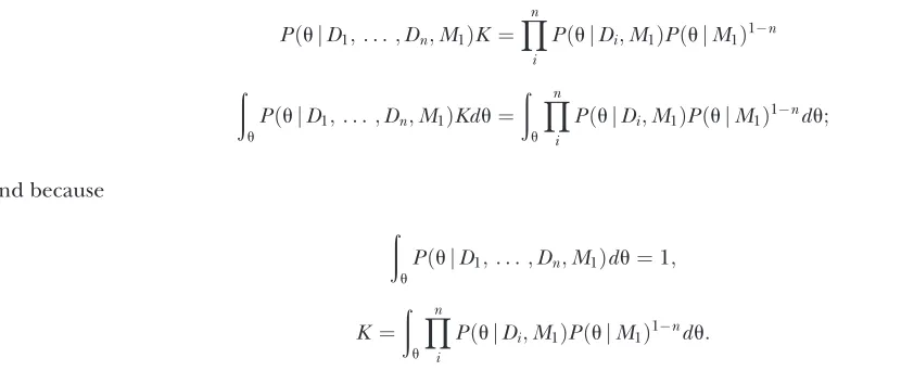
The denominator in (A2) can be built up during the MCMC run. The main difference between (A1) and (A2) is that the latter allows completely independent calculation for the unlinked loci and therefore allows easy distribution of the inference on a computer cluster or even computer grids, facilitating the analysis of data sets with many unlinked loci. The Bayesian inference offers a convenient tool for comparing different population models without requiring that models be nested. The marginal likelihoods are normally not computed during an MCMC run because these normalizing weights cancel in comparisons during the run. They need to be computed and recorded, however, when the combined marginal likelihoods need to be calculated; to do that we must evaluate the denominator of (A1):

PðD1;D2;. . .;DnjMiÞ ¼

ð

u

PðujMiÞ

Yn

i

PðDiju;MiÞdu: ðA5Þ

Theorem2.The combined marginal likelihoods over all independent data blocks can be calculated as a product of independently

calculated marginal likelihoods for each data block and a constant.

Proof. The combined estimator of the posterior distribution is

PðujD1;. . .;Dn;M1Þ ¼

PðujM1ÞQni PðDiju;M1Þ

PðD1;. . .;DnjM1Þ

: ðA6Þ

Converting the likelihoods using posteriors on the right,

PðujD1;. . .;Dn;M1Þ ¼

PðujM1ÞQni PðujDi;M1ÞPðDijM1Þ

PðujM1ÞnPðD1;. . .;DnjM1Þ

¼

Qn

i PðujDi;M1ÞPðDijM1Þ

PðujM1Þn1PðD1;. . .;DnjM1Þ ;

ðA7Þ

and movingP(D1,. . .,DnjM1) to the left andP(ujD1,. . .,Dn,M1) to the right results in

PðD1;. . .;DnjM1Þ ¼

Yn

i

PðDijM1Þ

Qn

i PðujDi;M1Þ

PðujM1Þn1PðujD1;. . .;Dn;M1Þ

: ðA8Þ

(13)

K ¼

Qn

i PðujDi;M1Þ

PðujM1Þn1PðujD1;. . .;Dn;M1Þ

: ðA9Þ

Moving the combined posterior and integrating both sides withuleads to a reexpression ofK,

PðujD1;. . .;Dn;M1ÞK ¼

Yn

i

PðujDi;M1ÞPðujM1Þ1n ðA10Þ

ð

u

PðujD1;. . .;Dn;M1ÞKdu¼

ð

u

Yn

i

PðujDi;M1ÞPðujM1Þ1ndu; ðA11Þ

and because

ð

u

PðujD1;. . .;Dn;M1Þdu¼1; ðA12Þ

K ¼

ð

u

Yn

i

PðujDi;M1ÞPðujM1Þ1ndu: ðA13Þ

This allows the calculation of the combined marginal likelihood using independent inferences

PðD1;. . .;DnjM1Þ ¼K

Yn

i

PðDijM1Þ: ðA14Þ

n

The denominator in (A2) is equivalent toKand has already been calculated during the MCMC run; it can be reused to calculate the combined marginal likelihoods.

Calculation of the scaling factorKin MIGRATE:In a Bayesian inference run of MIGRATE,Kis calculated from the recorded posterior probabilitiesP(ujDi) and the priorP(u) for a particular modelMwhereuare all the parameters of the model andDiis the data for each unlinked locus. For example, in a simple one-parameter scenario,u¼a, we record aand its prior during the MCMC run. Then we construct a histogram of thea-values that represents the posterior distribution P(ajD). The prior distribution is also calculated at the values of the histogram columns. Summing over the histogram corrected for the overuse of the prior approximates the integral and calculatesK. With a single locus,K¼1 and the "combined’’ marginal likelihood is the same as the single-locus marginal likelihood. With multiple parameters the integral will be multidimensional. If we assume that the parameters are independent of each other, the integration can be simplified. If we believe that the parameters are correlated, then we would need to calculate a multidimensional histogram; this is more tedious but certainly doable. MIGRATE uses the assumptions that parameters are independent because in our experience mutation-scaled migration rates and mutation-scaled population sizes are almost uncorrelated.

Specification of population models when some populations are isolated: MIGRATE uses two options to specify particular population models. The connection matrix allows the specification of directionality of gene flow, such as symmetric numbers of immigrants, symmetric immigration rates, average immigration rates, and immigration rates fixed to particular constants, for example, zero. If constants other than zero are used, then the start parameter settings need to be used in addition to the connection matrix to specify the values. This system allows approximating models where the populations are isolated from each other (Table 6) by inserting immigration rates that are very close to zero. For the humpback whale example we fixed all immigration rates to an isolated population as 100 times smaller than the mutation rate.

(14)

(15)

Supporting Information

http://www.genetics.org/cgi/content/full/genetics.109.112532/DC1