ABSTRACT
SHIN, JAEKWAN. Optimizing Product Line Offerings using Customer Preference Data. (Under the direction of Dr. Scott Ferguson).
In engineering design research the paradigm of market-based product design explores the integration of quantitative customer preference data and product design optimization problems. This method provides interdisciplinary approaches for connecting the marketing and engineering domains so that a diverse set of customer needs can be satisfied. This dissertation demonstrates that heterogeneous customer preferences models can be used to determine the most effective combination of product features in a product line optimization by exploring the formulation of effective product design search problems.
The first research topic addressed in this dissertation aims to understand the implication of consumer choice behavior and how the selection of a discrete choice model influences the results of a product design search problem. Motivation for this research topic comes from the challenges posed by Bayesian-based noncompensatory models. To overcome these challenges, the suitability of using a compensatory model in the presence of noncompensatory choices when conducting a product design search is explored.
The second research topic investigates how the choice of representing heterogeneous customer preferences effects the configuration of an optimal product line solution. Continuous and discrete representations of heterogeneity are available to design researchers, and the choice of model formulation can have a substantial impact on the final product design and the estimated values associated with different managerial objectives. The relative performance of each model form is compared in terms of model fitness and predictive ability. The structure of heterogeneous preferences is also explored to investigate why differences are observed in model estimates and product solutions obtained from an optimization.
sacrifice gap and an optimization problem formulation that can be used to identify the customizable product features in a mass customization environment.
The fourth research topic quantitatively defines the reliability and robustness of a product design under uncertainty in discrete choice methods. Ignoring uncertainties associated with customer preferences and their estimation has caused concern about the reliability and robustness of an optimal product design solution. This study leverages Randomized First Choice (RFC) simulations to address stochastic preference coefficients. Based on the RFC, a quantitative way of measuring reliability and robustness of a product line design is proposed. A multi-objective problem formulation is developed to integrate the stochastic aspects into one framework. Then, a multi-attribute decision method for handling conflicts in decision making is used to demonstrate how a decision maker can choose a single design from the set of solutions under tradeoffs in reliability and robustness.
Optimizing Product Line Offerings using Customer Preference Data
by Jaekwan Shin
A dissertation submitted to the Graduate Faculty of North Carolina State University
in partial fulfillment of the requirements for the Degree of
Doctor of Philosophy Mechanical Engineering
Raleigh, North Carolina 2016
APPROVED BY:
_______________________________ _______________________________
Dr. Scott Ferguson Dr. Larry Silverberg
Chair of Advisory Committee
_______________________________ _______________________________
BIOGRAPHY
ACKNOWLEDGMENTS
The author would like to acknowledge the support from the National Science Foundation through NSF Grant No. CMMI-0969961 and CMMI-1054208. Any opinions, findings, or conclusions presented in this dissertation are those of the authors and do not necessarily reflect the views of either of these organizations.
I would like to express my sincere gratitude to my advisor Prof. Scott Ferguson for the continuous support of my Ph.D. study and related research, for his patience, motivation, and immense knowledge. Besides my advisor, I would like to thank my dissertation committee members: Prof. Larry Silverberg, Prof. Gregory Buckner, and Prof. Jonathan Bohlmann for their insightful comments and encouragement.
My sincere thanks also go to Prof. Ikjin Lee who was my advisor at the University of Connecticut and Prof. Kunsoo Huh who was my master’s advisor at Hanyang University.
I thank my labmates in the System Design Optimization lab at North Carolina State University and Machine Monitoring and Control lab at Hanyang University. Also, I am grateful to the Korean students in the mechanical engineering department at NCSU.
TABLE OF CONTENTS
LIST OF TABLES ... viii
LIST OF FIGURES ... x
Chapter 1. Introduction ... 1
1.1. Motivation ... 1
1.2. Market-Based Product Design ... 1
1.3. Research Questions ... 3
1.4. Significance of Research Topics ... 4
1.4.1. Significance of Research Question 1 ... 5
1.4.2. Significance of Research Question 2 ... 7
1.4.3. Significance of Research Question 3 ... 8
1.4.4. Significance of Research Question 4 ... 9
1.5. Dissertation Outline... 10
Chapter 2. Background ... 12
2.1. Discrete Choice Models ... 12
2.2.1. Discrete choice analysis in market-based product design ... 12
2.2.2. Logit model ... 14
2.2.3. Latent class model... 15
2.2.4. Hierarchical Bayes mixed logit model ... 16
2.2. Optimization Techniques for a Product Line Design Problem ... 18
Chapter 3. Modeling Noncompensatory Choices with a Compensatory Model ... 21
3.1. Introduction ... 21
3.2. Background Knowledge ... 22
3.2.1. Noncompensatory choice models ... 22
3.3. Technical Approach ... 26
3.3.1. Synthetic choice data ... 26
3.3.2. Real choice data ... 28
3.4. Case Study using Synthetic Choice Data ... 30
3.4.1. Generating synthetic choice data ... 30
3.4.2. HB-MNP model with conjunctive rules ... 33
3.4.3. Latent class analysis ... 35
3.4.4. HB-ML model ... 37
3.4.5. Product design search ... 42
3.5. Case Study using Real Choice Data ... 47
3.5.1. Survey design and modeling ... 47
3.5.2. Product design search ... 48
3.6. Summary ... 50
Chapter 4. Implications of Heterogeneous Preference Presentation ... 52
4.1. Introduction ... 52
4.2. Technical Approach ... 53
4.2.1. Approach to validate model fitness and predictive ability... 54
4.2.2. Approach to investigate heterogeneity structure ... 55
4.2.3. Approach to investigate implications of model form choice ... 59
4.3. Case Study using Synthetic Choice Data ... 60
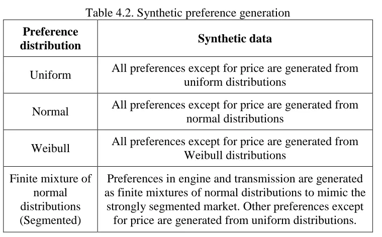
4.3.1. Synthetic preference and virtual survey ... 60
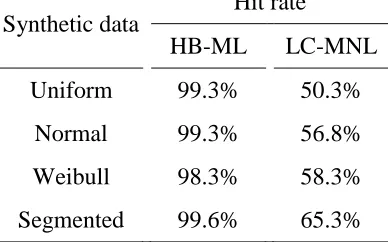
4.3.2. Validating model fitness and predictive ability using first-choice analysis ... 63
4.3.3. Validating model fitness and predictive ability using preference share analysis 65 4.3.4. Investigating heterogeneity structure using attribute importance ... 66
4.3.6. Investigating implications of model form choice ... 74
4.4. Case Study using Real Choice Data ... 76
4.4.1. Discrete choice design ... 76
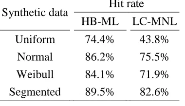
4.4.2. Validating model fitness and predictive ability ... 77
4.4.3. Investigating heterogeneity structure using attribute importance ... 77
4.4.4. Investigating heterogeneity structure using attribute level preference ... 79
4.5. Summary ... 83
Chapter 5. Quantifying Customer Sacrifice for Mass Customization Environments ... 85
5.1. Introduction ... 85
5.2. Quantitative Definition of Sacrifice Gap ... 88
5.2.1. Datum ... 88
5.2.2. Sacrifice gap... 89
5.3. Implications of Sacrifice Gap on Product Search Problem ... 92
5.3.1. Survey design ... 93
5.3.2. Respondent-level product search ... 93
5.3.3. Product line search ... 97
5.4. Mass Customization ... 102
5.4.1. Customization charge... 102
5.4.2. Constraints of design variables ... 103
5.4.3. Optimization procedure ... 103
5.4.4. Results ... 106
5.5. Summary ... 107
Chapter 6. Reliability and Robustness of Product Line Offerings under Uncertainty when Using Discrete Choice Methods ... 110
6.1. Introduction ... 110
6.2.1. Uncertainty in discrete choice methods ... 113
6.2.2. HB draws ... 116
6.2.3. Randomized first choice simulation... 116
6.3. Technical Approach ... 117
6.3.1. Reliability of a product design in market ... 118
6.3.2. Robustness of a product design in market ... 121
6.3.3. Product line design under uncertainty in discrete choice methods ... 122
6.4. Case Study ... 124
6.4.1. Generating synthetic choice data ... 124
6.4.2. Quantifying variation in demand model ... 125
6.4.3. Single-objective product line search ... 129
6.4.4. Multi-objective product line search considering reliability and robustness ... 133
6.5. Summary ... 138
Chapter 7. Conclusions ... 140
7.1. Research Summary ... 140
7.2. Discussion of Research Questions ... 140
7.2.1. Research Question 1 ... 140
7.2.2. Research Question 2 ... 141
7.2.3. Research Question 3 ... 142
7.2.4. Research Question 4 ... 143
7.3. Future Research Topics ... 144
BIBLIOGRAPHY ... 146
APPENDICES ... 157
APPENDIX A. MP3 player survey data and modeling result ... 158
APPENDIX B. Optimum product line solutions used in Chapter 4.3.6 ... 162
LIST OF TABLES
Table 3.1. Car attributes and levels used in virtual survey ... 31
Table 3.2. Pre-defined preferences of virtual respondents ... 31
Table 3.3. Attribute importance of the synthetic data ... 33
Table 3.4. Threshold estimates for the posterior means of the conjunctive model ... 34
Table 3.5. Part-worth estimates for the noncompensatory model ... 35
Table 3.6. Number of members in each group... 36
Table 3.7. Membership probability of belonging to a group ... 37
Table 3.8. Attribute importance of latent class analysis ... 37
Table 3.9. Part-worth estimates for the HB-ML model ... 38
Table 3.10. Hit rate comparison between HB-MNP with conjunctive rules and HB-ML model ... 39
Table 3.11. Zero-centered part-worth estimates of each segment obtained using HB-ML model ... 39
Table 3.12. Attribute importance of HB-ML model ... 41
Table 3.13. Part-worth comparison of the switched products ... 42
Table 3.14. Pricing structure ... 43
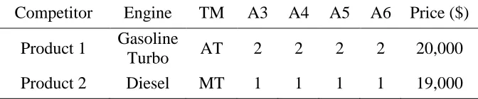
Table 3.15. Attribute levels of competitor products in the market ... 43
Table 3.16. Optimal product configuration for each model (Scenario 1) ... 44
Table 3.17. Optimal product configuration for each model (Scenario 2) ... 44
Table 3.18. Choice probability interval sensitivity study ... 46
Table 3.19. Optimal product configuration for each model (Scenario 1) ... 49
Table 3.20. Optimal product configuration for each model (Scenario 2) ... 49
Table 4.1. Attributes and levels used in virtual survey ... 61
Table 4.2. Synthetic preference generation ... 61
Table 4.3. Hit rate for the choice tasks used in the estimation ... 63
Table 4.6. RMSE of preference share ... 66
Table 4.7. KS test of Spearman correlation in feature importance ... 68
Table 4.8. KS test of Spearman correlation in feature level preferences ... 70
Table 4.9. Results of product line design optimization ... 74
Table 4.10. Analysis of product line design ... 75
Table 4.11. Hit rate comparison for real data ... 77
Table 4.12. Analysis of Spearman correlation coefficient of attribute level preference ... 82
Table 5.1. Function value of SG and SOP problems ... 95
Table 5.2. Function value of SG and SOP problems for each group ... 95
Table 5.3. Solution of product line search ... 97
Table 5.4. Group analysis of product line solution ... 98
Table 5.5. Product feature for the products in the zero-SG range ... 102
Table 5.6. Customization charge structure ... 103
Table 5.7. Optimum product feature solution for mass customization ... 106
Table 5.8. Comparison of mass customization solution ... 107
Table 5.9. Group-level comparison of mass customization solution ... 107
Table 6.1. Literature that consider uncertainty in demand model ... 114
Table 6.2. Tablet PC attributes and levels ... 125
Table 6.3. Data comparison ... 127
Table 6.4. Product line of each RFC data ... 129
Table 6.5. Pricing structure ... 129
Table 6.6. Attribute levels of competitor products in the market ... 129
Table 6.7. Deterministic optimal product line design ... 130
Table 6.8. Reliability and Robustness analysis ... 130
Table 6.9. Multi-objective solution comparison ... 136
LIST OF FIGURES
Figure 1.1. Framework of market-based product design ... 2
Figure 2.1. Discrete choice survey question (choice task) ... 13
Figure 2.2. Estimating part-worths from a discrete choice survey ... 13
Figure 2.3. Product design optimization ... 13
Figure 2.4. Flowchart of Genetic Algorithm ... 20
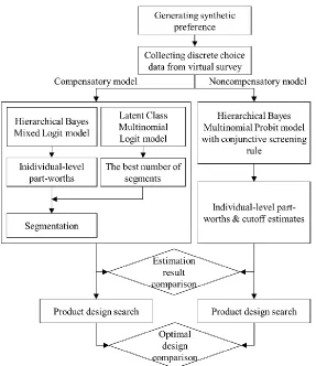
Figure 3.1. Flowchart for comparing compensatory models and a Bayesian-based noncompensatory model with conjunctive screening rules for synthetic choice data ... 27
Figure 3.2. Conceptual procedure of noncompensatory choice simulation using hypothetical screening rules ... 28
Figure 3.3. An example of a hypothetical noncompensatory choice simulation when using discrete choice data obtained from an actual survey ... 29
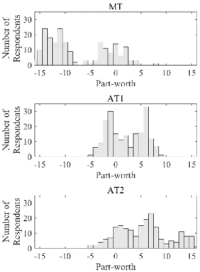
Figure 3.4. Histogram of aggregate posteriors for transmission attribute obtained using the HB-ML model ... 40
Figure 3.5. Conceptual diagram to show the absence of a strict threshold in compensatory modeling of noncompensatory choice ... 42
Figure 3.6. Interval comparison between the max. and min. choice probabilities of each attribute ... 46
Figure 4.1. Strategy for model comparison ... 54
Figure 4.2. Strategy for validating predictive ability: (a) First-choice analysis (b) Preference share analysis ... 55
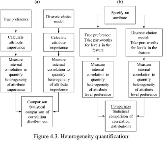
Figure 4.3. Heterogeneity quantification: (a) Internal heterogeneity of attribute importance (b) Internal heterogeneity of attribute level preference ... 56
Figure 4.4. Strategy for investigating implications of model form choice for product line design ... 59
Figure 4.6. CDF of preference share error: (a) Uniform (b) Normal (c) Weibull (d) Finite
mixture of normal distribution (Segmented)... 65
Figure 4.7. Histogram of correlation coefficient quantifying heterogeneity in feature importance (Synthetic data: Uniform distribution) ... 67
Figure 4.8. Visual comparison of CDFs for importance heterogeneity ... 68
Figure 4.9. Q-Q plot of attribute importance heterogeneity ... 69
Figure 4.10. Visual comparison of CDFs for level preference heterogeneity (Synthetic data: Uniform distribution) ... 72
Figure 4.11. Q-Q plot of level preference heterogeneity (Synthetic data: Uniform distribution) ... 73
Figure 4.12. Comparison of HB-ML and LC-MNL models using attribute importance correlation (a) Histogram of correlation coefficient of HB-ML model (b) Histogram of correlation coefficient of LC-MNL model (c) Empirical CDFs ... 78
Figure 4.13. Attribute 1. Comparison of HB-ML and LC-MNL models using feature level preference structures: (a) Histogram of correlation coefficient of HB-ML model (b) Histogram of correlation coefficient of LC-MNL model (c) Empirical CDFs... 80
Figure 4.14. Attribute 4. Comparison of HB-ML and LC-MNL models using feature level preference structures: (a) Histogram of correlation coefficient of HB-ML model (b) Histogram of correlation coefficient of LC-MNL model (c) Empirical CDFs... 81
Figure 5.1. Representations of sacrifice gap: (a) using utility differences (b) using odd ratios ... 90
Figure 5.2. Conceptual diagram of product utilities in sacrifice gap metric ... 92
Figure 5.3. Utility comparison of SG optimum designs for Group B ... 95
Figure 5.4. Price importance: (a) Group A (b) Group B ... 96
Figure 5.5. Sacrifice gap difference versus preference share: (a) SG optimization for Group A (b) SG optimization for Group B (c) SOP optimization for Group A (d) SOP optimization for Group B ... 99
Figure 5.6. Respondent-level analysis of two product line solutions ... 101
Figure 6.1. Variability in hypothetical solutions: (a) Single-objective (b) Multi-objective 112
Figure 6.2. Visualization of Failure I for a Single RFC Replicate ... 119
Figure 6.3. Visualization of Failure II for a Single RFC Replicate ... 120
Figure 6.4. Robust design Type I (Chen et al. 1996) ... 122
Figure 6.5. Flowchart of the presented study ... 124
Figure 6.6. Variability in performance function ... 131
Figure 6.7. Distributed FCS and probability of Failure II: (a) Solution A (b) Solution B (c) Solution C (d) 95% confidence ellipse ... 132
Figure 6.8. Pareto design alternatives of product line search problem: (a) 3-D plot (b) FCS vs SD of FCS (c) FCS vs Prob. of Failure II (d) SD of FCS vs Prob. of Failure II ... 134
Figure 6.9. Refined design solutions... 135
Chapter 1. Introduction
1.1. Motivation
The success of a product depends on making the correct decisions during the design process. Recent smartphone sales give a representative example of how product design decisions can play a central role in product success. The iPhone 6 and iPhone 6 plus launched in September 2014. These phones had larger screens than the iPhone 5 and 5s series. Apple announced it sold 46% more devices (74.5 million) during the holiday season in 2014 than the record 51 million iPhone 5s sold that quarter the year earlier (Apple Press Release 2015). This was the most successful quarter in Apple’s business history. To explain this success, many analysts said the key factor was the larger screens and multiple sizes. The design decision to adopt two variants with larger screens has made a significant contribution to the success of these new models. This leads to the following question. How can information about customer preference be used to make the most effective design decisions?
In a globally competitive market, a significant challenge for a company is understanding consumer preferences and leveraging that information to guide the introduction of desired products. The paradigm of market-based product design explores the integration of quantitative customer preference data and product design optimization problems. This method provides interdisciplinary approaches for connecting the marketing and engineering domains so that a diverse set of customer needs can be satisfied. The work completed in this dissertation demonstrations that heterogeneous customer preferences models can be used to determine the most effective combination of product features in a product line optimization by exploring the formulation of effective product design search problems.
1.2. Market-Based Product Design
using statistical techniques to create demand models; third, a product design search problem is formulated and optimization techniques are used to identify optimal product attributes associated with managerial objectives and subject to pre-defined constraints.
Figure 1.1. Framework of market-based product design
The first two stages of this process involve predictive market modeling, as are viewed as preprocessing steps for the product design search problem, as shown schematically in Figure 1.1. As one of the tools for estimating customer preferences, discrete choice analysis has been widely used by implementing variations of the generalized linear model - such as logit and probit models (Chen, Hoyle, and Wassenaar 2013; Train 2009). Recently, models that represent preference heterogeneity – providing the ability to represent variation in taste across individuals (Allenby and Rossi 1998) – have seen greater use.
Product design formulations can have many variants according to the managerial objectives and design constraints considered. In a product line optimization formulation, the design variable X can be defined as discrete numbers to encode product attributes. The objective function F(X) is typically defined as profit or preference share. Design constraints such as design infeasibility can be defined if needed. Overall, these problems often require discrete and mixed-integer problem formulations, leading to the use of heuristic optimization techniques. Genetic Algorithms (GA) have been shown to have advantages in that they require far fewer function evaluations to converge to a set of solutions that other methods (e.g. grid searches, iterative weighted sums). In addition, a GA is very robust to ill-conditioned problem formulations (discontinuous, discrete, etc.). Details about optimization techniques for the problem are discussed in Chapter 2.2.
1.3. Research Questions
This dissertation is focused on theoretical frameworks for supporting design decisions in product development by integrating customer preference data into design optimization problems. The objective of this dissertation is to explore how heterogeneous preference estimates can be used in product design optimization. The research topic can be classified into two broad categories: investigating how the selection of discrete choice model influences the optimal product line configuration, and developing design search methods under preference heterogeneity. The research questions explored in this work are summarized as:
Research Question 1. When respondents make noncompensatory choices with conjunctive screening rules, how does the optimal product line solution differ when preferences are modeled using compensatory and noncompensatory models? (Chapter 3)
Research Question 3. How can sacrifice gaps be quantified to formulate an optimization problem for mass customization environments? (Chapter 5)
Research Question 4. How can the reliability and robustness of a product design be defined under uncertainty when using discrete choice methods, and how was these measures be used to support engineering design decision-making? (Chapter 6)
Research Question 1 is focused on investigating the limitations of the Bayesian-based noncompensatory models in design optimization problems, and exploring the feasibility of using a compensatory model when respondents make noncompensatory choices. In Research Question 2, continuous and discrete representations of heterogeneous preferences are empirically compared in the context of an optimal product line solution. Research Question 3 proposes a quantitative definition of customer sacrifice gap and develops a design problem formulation for mass customization environments. Research Question 4 explores how uncertainty can be managed when using discrete choice methods, and a multi-objective optimization problem considering the reliability and robustness of a product design is proposed.
1.4. Significance of Research Topics
1.4.1. Significance of Research Question 1
Many forms of the discrete choice models used in market-based design assume that consumers make compensatory choices. Compensatory choices are based on an additive utility rule; that is, high levels on some features can compensate for low levels on other features. However, a number of papers have demonstrated that noncompensatory choice models often improve both model realism and accuracy in predicting consumers’ choices (Desai and Hoyer 2000; Ding 2007; Erdem and Swait 2004; Gilbride and Allenby 2006). The noncompensatory choice rule supposes consumer’s choice tasks are conducted using heuristic decision-making strategies.
Imagine a consumer, who does not want a manual transmission, shopping for a new car. The consumer first narrows his choices to a small set of cars equipped with an automatic transmission and then compares the cars in that set using an additive rule. This choice behavior is called a consider-then-choose process. The presence of a noncompensatory preference structure in the first stage forms a consideration set. The second stage compares product alternatives and selects one from this set, reflecting a compensatory choice. When designing products for noncompensatory consumers using a consider-then-choose process, one of the most significant challenges is launching products that are not being screened out of the consideration set.
Since the early 2000s, there has been increased development in modeling noncompensatory choices using computationally expensive methods like Bayesian inference and machine learning techniques. The performance of noncompensatory models has been proven in terms of model fitness and predictability by several other research projects (Arora et al., 2011; Gilbride and Allenby, 2004; Jedidi and Kohli, 2005; Swait, 2001; Yee et al., 2007). It has been shown that noncompensatory models can slightly outperform compensatory models in both hit rate for holdout tasks and likelihood function values.
system design problems to deal with the discontinuous likelihood functions of a consider-then-choose model (Morrow, Long, and MacDonald 2014). Long and Morrow investigated the impact of noncompensatory choice behavior when an optimal design was created using compensatory models (Long and Morrow 2014). Their studies, however, have been focused on evaluating predictive power and design error at the population-level without exploring individual-level part-worth estimates.
Research Question 1 is motivated by the potential challenges of the existing Bayesian-based noncompensatory model. These challenges include:
Inadequate screening rule assumptions that may lead to an incorrect estimation of noncompensatory choices because the existing noncompensatory models are derived with specific screening rules.
Aggregate part-worths have an inappropriate form that is difficult to use in optimization problems due to their probabilistic cutoff values.
Discontinuous choice probability functions associated with noncompensatory models can cause numerical difficulty when precisely solving design constraints during optimization using a GA.
Considering these limitations, compensatory models may be a more suitable form for optimization problem formulations because they have valuable advantages that include:
Compensatory models have generalized forms not affected by heuristic rules. Aggregate part-worths can be integrated into optimization problems.
Likelihood functions are described as continuous functions using logistic or normal distributions.
question, the suitability of the Bayesian-based compensatory modeling of noncompensatory choices is investigated.
1.4.2. Significance of Research Question 2
Effectively designing products for a market requires the modeling of variation in taste across individuals. Representing such variation in taste is significant because capturing different segments of the market leads to differentiated product design (Allenby and Rossi 1998). Two customer preference models capable of representing customer heterogeneity are the hierarchical Bayes mixed logit (HB-ML) model and the latent class multinomial logit (LC-MNL) model. The HB-ML model estimates part-worth values by assuming a continuous distribution of preference heterogeneity. The LC-MNL model describes heterogeneity with discrete distributions that are determined by assigning the probability that a respondent belongs to a particular class.
The two representations available to model preference heterogeneity can have a substantial impact on the final product design and the managerial objective. However, the impact of preference heterogeneity on product configuration has not received much attention in the market-based product design literature. Michalek et al. (2011) maintained that even though discrete choice models with continuous and discrete heterogeneity representations can predict choices almost equally well (Andrews et al., 2002a; Andrews et al., 2002b), the optimized designs from different models may be very different. In a recent study by Sullivan et al. (2011), part-worth estimates from both models were used to design an optimal product line. Significant differences between the design solutions were observed. Sullivan et al. (2011) explored why the solution differed by comparing correlations between the part-estimates and simulating first-choice at the respondent level.
1.4.3. Significance of Research Question 3
Mass customization is a product strategy that provides custom-tailored goods or services to meet a consumer’s diverse needs at near mass production prices (Gilmore and Pine 2000; S. M. Ferguson, Olewnik, and Cormier 2014). When done correctly, mass customization is a win-win strategy for both customers and producers. Consumers can get a tailor-made product at a reasonable price that reflects their personal selection of product features. Producers can make their products more appealing to consumers by obtaining more accurate information about demand and saving costs by eliminating waste in their supply chains.
The term ‘mass customization’ was first used by Davis (1987) nearly 30 years ago, where mass customization was explained as having the capability of reaching the same number of customers as in a mass market while treating those customers “individually as in the customized markets of pre-industrial economies. (Davis 1987)” Later, Pine (1999) described mass customization as “providing tremendous variety and individual customization, at prices comparable to standard goods and services” to fill the market “with enough variety and customization that nearly everyone finds exactly what they want.” From a manufacturing perspective, Du et al. (2001) describe mass customization as “the technologies and systems to deliver goods and services that meet individual customers’ needs with near mass production
efficiency.” All definitions of mass customization are consistent in that they share two notions: 1) they discuss that customer needs can be met more effectively using customized product offerings, and 2) they aim to leverage innovation in product design, manufacturing, and logistics to maintain prices comparable to mass produced products. In this context, the benefit of mass customization is its ability to simultaneously increase value to both the customers and the company when compared to mass production.
i. Limitations of existing customer needs and preference assessment tools.
ii. The need to explore approaches for requirement specification and conceptual design. iii. Insights from methodologies focused on the development of durable mass
customization goods.
iv. Necessary enhancements in information mapping and handling.
Among the research opportunities, a tool for customer needs and preference assessment is important at the early stage of product development (S. M. Ferguson, Olewnik, and Cormier 2014). However, despite advancements in consumer research, a quantitative assessment tool of customer preference has yet to be developed for mass customization environments. In particular, although conceptual definitions of the sacrifice gap exist, a process for obtaining a quantitative measure of the term is almost unexplored. Research Question 3 aims to quantitatively define sacrifice gap and develop an optimization problem formulation capable of identifying the optimal mix of customizable product features for mass customization environments.
1.4.4. Significance of Research Question 4
Critical limitations of existing market-based product design methods arise from the common assumption that customer preferences are inherently deterministic. This occurs in spite of the fact that they are statistical estimates exhibiting estimation error. Existing approaches use point estimates of an individual’s part-worths in market simulations, ignoring variability in these estimates. Therefore, a critical issue when solving product design search problem becomes the reliability and robustness of the optimal design under uncertainty.
approximation (SAA) method for stochastic discrete optimization (Kleywegt, Shapiro, and Homem-de-Mello 2002) to the share-of-choice product-line problem. They suggested that a solution’s uncertainty could be managed by taking a sufficient number of draws per person. Wang and Curry (2012) studied the concept of robustness in integer programming for the share-of-choice problem. They assumed that individual preferences are bounded, independent, and symmetric variables. In addition, the covariance matrix for individual level part-worths was assumed to be a diagonal matrix, preventing correlation among product features. However, these assumptions do not agree with their random-effects model estimated using the hierarchical Bayes technique. In a mixed logit model, no constraint exists on the covariance matrix and preference coefficients are not defined as interval variables.
To answer this question, a multi-objective optimization problem formulation is proposed for reliable and robust product line designs. Demand model variability is quantified using a Randomized First Choice (RFC) method. Robustness and reliability of market-based product design are defined and integrated into one framework. A multi-attribute decision method is then conducted to support design decision-making from the set of candidate solutions.
1.5. Dissertation Outline
Chapter 2. Background
2.1. Discrete Choice Models
Discrete choice analysis is used to create models of product demand by capturing customer’s choice behavior in a series of choice questions (Louviere and Woodworth 1983). In most market-based product design research, consumer preferences are estimated using discrete choice models with a compensatory utility rule. The assumption behind this compensatory utility rule is that consumers weigh and make trades between attributes when making a purchasing decision. Product utility is calculated by adding the part-worth estimates associated with each product feature selected.
The necessary background knowledge about discrete choice models and their ability to represent customer heterogeneity is introduced in Chapter 2.2. Chapter 2.2.1 provides the overview of discrete choice methods to build predictive market models. Chapter 2.2.2 introduces the fundamentals of discrete choice models and logit models. Chapter 2.2.3 and 2.2.4 review Latent Class Multinomial Logit (LC-MNL) model and Hierarchical Bayes Mixed Logit (HB-ML) model, which are called as discrete and continuous representations of preference heterogeneity, respectively.
2.2.1. Discrete choice analysis in market-based product design
The survey technique used in Discrete Choice Analysis (DCA) is designed to closely mimic the purchase process of buyers in the real world – choosing among available offerings including a ‘no-buy’ option. The main characteristics distinguishing DCA from conventional conjoint value analysis (Orme 2006) is that respondents express preferences by choosing from sets of design concepts, rather than by rating or ranking each concept individually.
DCA consists of three core tasks:
Figure 2.1. Discrete choice survey question (choice task)
Estimate part-worths: Determine the value respondents place on each feature by exploring the trade-offs they make (Figure 2.2). Chapters 2.2.2, 2.2.3, and 2.2.4 describe mathematical details about how to define and estimate part-worth values.
Figure 2.2. Estimating part-worths from a discrete choice survey
Market simulation: Simulate how the market reacts to various feature trade-offs you are considering. ‘What-If’ scenarios can be tested in an optimization problem to predict the choice probability of a hypothetical design (Figure 2.3).
2.2.2. Logit model
While conventional conjoint value analysis uses a linear regression to estimate part-worth utilities, DCA is mathematically based on the logistic regression of a utility function. A utility function is a mapping of a multi-dimensional attribute space into a single dimensioned choice probability space. A basic assumption is that each customer’s choice decision can be modeled by a choice utility that person n obtains from the alternative j. This choice utility can be expressed as a sum of an observed utility Vnj and an unobserved random disturbance nj as in (Train 2009; Ben-Akiva and Lerman 1985; Chen, Hoyle, and Wassenaar 2013; Rossi, Allenby, and McCulloch 2005).
T
nj nj nj n nj nj
U V x (2.1)
In this equation, n is a vector of part-worths for the nth individual and xnj is a vector of values that describes the configuration of product j. In generalized form, n and ni are expressed as n n* and
*
ni ni
, where is a scale parameter that is typically set to 1. Usually, n is unknown to the researcher and estimated statistically.
The probability that decision maker n chooses alternative i in a binary choice scenario is defined by (Train 2009)
ni ni nj
ni nj nj ni
P P U U j i
P V V j i
(2.2)
derived given assumptions on the joint distribution of the unobserved utility. The choice probability (Pni) that a person n chooses an alternative i from a set of products j where
{1 }
j J can be obtained from the logit formula as (Train 2009)
T n ni
T n nj
x
ni x
j
e P
e
. (2.3)The choice probability is also known as preference share. For the multinomial logit model to estimate population-level preference, the part-worths are usually estimated using maximum likelihood estimation.
While compensatory models using an additive utility rule have been widely used due to their simplicity, the same models also impose several limitations. First, the additive utility rule may not accurately model real choice behavior because respondents often find it challenging to consider the entire set of product attributes when making a choice. Second, IIA (independence from irrelevant alternatives) becomes a challenge in compensatory models because the choice probability of an alternative is affected by the presence of other alternatives. This issue arises from the i.i.d. assumption of the error term ni. Third, part-worth estimates and choice probabilities are sensitive to changes in model parameters, such as the scale parameter .
2.2.3. Latent class model
(DeSarbo, Ramaswamy, and Cohen 1995). In the design community, latent class analysis has been used as a tool for market segmentation by Besharati et al. (2006), Williams et al. (2008), and Turner et al. (2011).
Since a multinomial logit model is used to evaluate the likelihood of each subgroup, it is called an LC-MNL model. An LC-MNL model first classifies individuals into segments with similar preferences and then estimates the part-worths of each segment using a multinomial model. Simultaneously, individuals’ probabilities of membership ( ) s in each segment are estimated (DeSarbo, Ramaswamy, and Cohen 1995). The unconditional choice probability
( )
P j that a respondent chooses an alternative j is obtained as
1
( ) ( ) ( )
S
s
P j s j s
(2.4)where ( )s is the probability of a respondent belonging to the class s, and ( j s) is the probability of a respondent choosing alternative j conditioned on belonging to the class s.
2.2.4. Hierarchical Bayes mixed logit model
Kannan, and Azarm 2011; Shiau et al. 2007; Foster et al. 2014; Hoyle et al. 2011; Michalek et al. 2011; Grace Haaf et al. 2014).
The mixed logit probability can be obtained as the integrals of multinomial probabilities over a density of part-worths and is derived as Eq. (2.5). The individual-level part-worths, n , are assumed as a multivariate normal distribution with density
b W,
and the parametersb and W are determined in estimation. However, analytic integration is impossible for the mixed logit probability because the multivariate distribution doesn’t have a closed-form. Thus, numerical integration is employed using Bayesian inference with Markov-Chain Monte-Carlo (MCMC) methods.
,
T ni T nj x ni x j eP b W d
e
. (2.5)The mixed logit model employing Bayesian inference is called a Hierarchical Bayes Mixed Logit (HB-ML) model because there are two levels. The assumption at the higher level is that an individual’s preferences are normally distributed. At the lower level, a logit formula in assumed to quantify the choice probability. With this hierarchy, the posterior distribution of Bayes’ rule for n, b, and W is expressed as (Train 2009):
, , n
n n
n ,
,
n
K b W n Y
L y b W k b W (2.6)where the chosen alternatives for person n are denoted yn and the choice of the entire sample are labeled Y{ ,y1 , y }N . ( , )k b W is the prior of b and W which are the parameters of
n b W,
that represents preference heterogeneity. L y
n n
is the likelihood function ofusing Gibbs sampling, draws of the posterior can be generated (Train 2009). Detailed procedures of the numerical integration are not presented in this dissertation.
In practical use, aggregate part-worths values are often used by taking the mean value from a finite numbers of draws r1, 2, ,R obtained from the distribution ofn. A corresponding aggregate choice probability is obtained as (Chen, Hoyle, and Wassenaar 2013)
, , , 1 1 1 1 ˆ T n r ni
T n r nj
x
R R
ni ni r x
r r
j
e
P P
R R e
(2.7)where R is the number of random draws, Pni r, is the probability of respondent n choosing
product i in the r th draw, and n r, is the corresponding simulated random coefficients.
However, using aggregate part-worths ignores sources of uncertainty associated with discrete choice methods, raising concerns about the reliability and robustness of optimal designs obtained when using market simulations.
2.2. Optimization Techniques for a Product Line Design Problem
Design optimization is a process of finding the best solution that satisfies design objectives under constraints. In market-based product design, the product line design problem using individual-level part-worths can be expressed as
1 1
1 1 ˆ
minimize Preference Share =
with respect to X = Product configurations
of own offerings in a product line
subject to lower and upper bounds of each a
N I
ni n i
P N I
ttribute
I and N indicate the number of products offered by a manufacturer and the number of respondents, respectively. ˆPni is the probability that respondent n chooses a product alternative i. Eq. (2.8) is a simplified representation of a product line search problem and many variants could be further developed. A product designer seeking an opportunity to adopt a market-based product design strategy would need to reflect limitations and decisions concerned with manufacturing, marketing, or engineering design. Design problems should be able to control any of these limitations and decisions in product feature configuration. In the design optimization problem, the limitations and decisions associated with these different aspects of the design problem can be specified as design variable constraints.
Many times the formulation of a product line design problem is combinatorial in nature. This leads to a mathematical optimization problem where an optimal solution is found from a finite set of objects. This specific type of combinatorial optimization problem is considered a computationally intractable (i.e., non-deterministic polynomial (NP) hard) problem, which means exact algorithm like integer programming and branch-and-bound (X. (Jocelyn) Wang, Camm, and Curry 2009) struggle to efficiently solve large-scale problems (Kohli and Sukumar 1990; Green and Krieger 1985).
Figure 2.4. Flowchart of Genetic Algorithm
A genetic algorithm, first introduced by (Holland 1975), is a type of evolutionary algorithm that is based on the Darwin’s natural selection theory. A typical genetic algorithm usually consists of four main steps: initialization, selection, crossover, and mutation as shown in Figure 2.4. Initialization is primarily focused on developing the initial population. Often, the initial population is randomly generated because priori information about the global optimum is usually not known. In product line optimization, generating a targeted population for a genetic algorithm using an individual’s preference estimates can reduce computational cost and improve solution quality (Foster et al. 2014). Selection specifies which designs in the population are chosen for the genetic operators (crossover and mutation). Then, the genetic operators update designs to generate a new design set. Finally, the algorithm should stop if the pre-defined termination condition is satisfied.
Chapter 3. Modeling Noncompensatory Choices with a Compensatory Model
The main goal of this chapter is to explore the quality of solution obtained to a product line design search when using a compensatory model in the presence of noncompensatory choices and a noncompensatory model with conjunctive screening rules. Motivation for this work comes from the challenges posed by Bayesian-based noncompensatory models: the need for screening rule assumptions, probabilistic representations of noncompensatory choices, and discontinuous choice probability functions. This chapter demonstrates how respondents making noncompensatory choices with conjunctive rules can lead to compensatory model estimations with distinct respondent segmentation and relative, large absolute part-worth values. Results from a product design problem suggest that using a compensatory model can provide benefits of smaller design errors and reduced computational costs. Product design optimization problems using real choice data confirm that the compensatory model and the noncompensatory model with conjunctive rules provide comparable estimates of a product not being screened out in a hypothetical noncompensatory choice simulation. While many different noncompensatory heuristic rules exist, the presented study is limited to conjunctive screening rules.
3.1. Introduction
minimum level for a product feature, and the customer will screen out a product that doesn’t meet the minimum level. This study is motivated by the inherent challenges associated with making screening assumptions and correctly inferring the screening rules used by a respondent population. Even when these screening rules can be correctly inferred, estimating a two-stage model can be challenging, leading to errors that can ultimately lead to sub-optimal design decisions. Further, optimization of a product line is made difficult because of the probabilistic representations of noncompensatory choice and the discontinuous choice probability functions that often accompany noncompensatory models.
One would need to know or be able to infer the screening rules in order to appropriately use a noncompensatory model. Even with adequate data with the screening rule assumption, errors associated with noncompensatory choice estimation could lead to sub-optimal design decisions. The suitability of using existing noncompensatory models is discussed in Chapter 3.2.1 by reviewing the existing models. In particular, Chapter 3.2.2 addresses the limitations of an existing noncompensatory model. Chapter 3.3 describes how to explore the performance of using a compensatory model in the presence of noncompensatory choices. This concept is examined in Chapter 3.4 by analyzing synthetic data. Chapter 3.5 deals with real choice data to explore differences in a product optimization using both the compensatory and noncompensatory models.
3.2. Background Knowledge
Compensatory models capable of estimating individual-level part-worths are described in Chapter 2.1. In Chapter 3.2, various heuristics of noncompensatory choices and their modeling methods are reviewed, mainly focusing on the HB multinomial probit model with conjunctive screening rule.
3.2.1. Noncompensatory choice models
because of its added realism. By employing noncompensatory screening rules, consumers narrow their decisions to a small set of products called a consideration set. Then, they use a compensatory choice rule to evaluate the remaining products and make a selection.
Various heuristic decision rules for noncompensatory choices have been proposed, including conjunctive, disjunctive, lexicographic-by-aspect, elimination-by-aspects, and disjunctions of conjunctions (Hauser 2009). The existing studies about the Bayesian-based noncompensatory models (Gilbride and Allenby 2006; Gilbride and Allenby 2004) suggest the conjunctive rule model is effective in both model fitness and predictability at individual-level estimates. Hence, this article focuses on consider-then-choose models with the conjunctive screening rule, where consumer consider if the product has all “must have” and no “must not have” aspects. It is formed by multiplying an indicator function across the attribute of an alternative as in Eq. (3.1) (Gilbride and Allenby 2004):
I(im m) 1
m
l
(3.1)Here, lim is the level of attribute m for choice alternative i. The cutoff value m, is the smallest level of the attribute that needs to be present for the consumer to consider the alternative (Swait 2001). The indicator function indicates whether a choice alternative is screened out or not in a noncompensatory choice. Thus, the indicator function, I( ) , is equal to 1 when a level lim exceeds a threshold value
m, and this indicates the choice alternative i is not screened out by a conjunctive rule in a noncompensatory choice. If the alternative has a lower level of the attribute than the cutoff value, the product is screened out.
Prob for all such that ( ) 1
ni ni nj m njm nm
P U U j
I l (3.2)njm
l is the level of the attribute for respondent n for alternative j and attribute m.
nm is a respondent-level threshold of attribute m for respondent n. When an attribute is continuously distributed, it is assumed that the cutoff values are normally distributed. When an attribute consists of discrete levels, a multinomial distribution can be adopted such that~ Multinomial( )
nm m
, where
m is the vector of multinomial probabilities associated with the grid for attribute m. Each level is tested to determine the highest possible cutoff value*
(nm) from allowable cutoff values (nmla ) using the Metropolis-Hastings algorithm (Kruschke 2010) based on a probability given in Eq. (3.3) (Gilbride and Allenby 2004) where l indicates attribute levels:
( )
with probability
( )
a
a nml ml
nm nml a
nml ml l
I I (3.3)This model returns an individual’s part-worths, cutoff values, and cutoff probabilities at each draw. Disjunctive and elimination-by-aspects rules can also be modeled using Bayesian inference (Gilbride and Allenby 2006; Gilbride and Allenby 2004).
The choice probabilities can be expressed as (J1) -dimensional integrals over the differences between the errors because probit models are not closed form (Train 2009). These differences are defined as Vnij Vni Vnj and nij ninj. Then, for the consider-then-choose process using a probit model the choice probability that individual n chooses any alternative
i that is in the consideration set is given by Eq. (3.4) (Gilbride and Allenby 2004)
( nij nij 0 ) ( n) n n
ni
V j i d j C
( )
I is an indicator of whether the statement in parentheses holds,
( )n is the joint normal density with zero mean and covariance , and Cn denotes a consideration set of a consumern.
Notice that noncompensatory attributes used to form consideration sets are excluded from part-worth estimation. In other words, noncompensatory attributes are only used to determine whether a choice alternative is in a consideration set in the first stage. Only compensatory attributes are used in part-worth estimation. This is because calculating the choice probability relies on the utility difference obtained by an additive utility rule. Noncompensatory attributes are used to estimate the probability of cutoff based on Eq. (3.3).
3.2.2. Challenges of using noncompensatory models
The performance of noncompensatory models has been proven in terms of model fitness and predictability (Gilbride and Allenby 2004; Gilbride and Allenby 2006; Swait 2001; Arora, Henderson, and Liu 2011; Jedidi and Kohli 2005; Yee et al. 2007). However, from the standpoint of design optimization, noncompensatory models have some inherent limitations:
Inadequate screening rule assumptions may lead to an incorrect estimation of noncompensatory choices. Further, there is no general form to describe all noncompensatory heuristics. For example, the HB-MNP model with conjunctive screening rules can only describe choices that screen out attribute levels lower than the minimum requirements. This form may be inappropriate for non-incremental levels such as color or brand.
Discontinuous choice probability functions (Eq. (3.4)) can cause numerical difficulty when precisely solving design constraints (Morrow, Long, and MacDonald 2014).
Considering these limitations, compensatory models have numerous advantages from a product optimization perspective: 1) generalized forms, 2) aggregate part-worths can be used, and 3) likelihood functions are continuous. Further, when estimating part-worths at the individual-level, large absolute part-worth values (relative to the other part-worth values estimated in a zero-centered formulation) can cause the additive part-worth rule to act like a noncompensatory rule (Hauser 2009). For these reasons, this article explores the challenges of using noncompensatory models and compares the results of a product optimization to those obtained when using compensatory models in the presence of noncompensatory choices.
3.3. Technical Approach 3.3.1. Synthetic choice data
The study explores how compensatory models can approximate a two-stage choice process, and examines the differences in an optimal design search when using compensatory and noncompensatory models. This approach is driven by the hypothesis that distinct population segments can be identified from the individual-level part-worths for specific attributes where noncompensatory decisions might be made. To verify this hypothesis, a two-stage process using the LC-MNL and HB-ML models is proposed, as shown in Figure 3.1.
of membership probability and the attribute importance. Then, the obtained segments are evaluated using individual part-worths in terms of attribute importance and heterogeneity representation.
3.3.2. Real choice data
Real choice data does not provide information about which respondents actually made noncompensatory choices, or what heuristics they used to make those choices. Thus, it is impossible to apply the same technical approach used to analyze the outcomes from synthetic choice data because ‘true’ preferences are not available. For this reason, a different approach is proposed to assess and compare the optimum product designs of compensatory and noncompensatory models, as shown in Figure 3.2. To assess and compare the optimum product designs of compensatory and noncompensatory models, a hypothetical noncompensatory choice simulation is proposed.
Figure 3.2. Conceptual procedure of noncompensatory choice simulation using hypothetical screening rules
out at the noncompensatory choice stage. This likelihood is easily obtained by dividing the number of feasible screening rules by the total number of choice simulations.
An example of a hypothetical noncompensatory choice simulation when using real choice data is shown in Figure 3.3. Assume that respondents took a discrete choice survey consisting of 10 choice tasks involving products with 2 attributes and 5 total levels (three for attribute 1 and two for attribute 2). The data in Figure 3.3 shows the cumulative number of times each attribute level was chosen in the 10 choice tasks. For Product 1, created using level L3 of attribute A1 and level L1 of attribute A2, it is clear that this product was not screened out because the respondent chose these two attribute levels at least once when completing the choice tasks. However, for Product 2, created using level L1 of attribute A1 and level L1 of attribute A2, the analysis is more complicated.
Figure 3.3. An example of a hypothetical noncompensatory choice simulation when using discrete choice data obtained from an actual survey
occur after the consideration set has been created. Hence, when running a simulation for several screening rules, the minimum likelihood that a product is not screened out can be estimated in the hypothetical noncompensatory choice simulation.
3.4. Case Study using Synthetic Choice Data
As shown in Figure 3.3, choice data itself cannot be used to explicitly state respondents’ choice processes. It is impossible to know who made noncompensatory choices and what heuristics were used. However, this information can be captured if synthetic data is created using pre-defined virtual agents. In this study, virtual respondents are generated using conjunctive screening rules because the existing studies of the Bayesian-based noncompensatory models suggest that the conjunctive rule model shows the best performance in both model fitness and predictability at individual-level estimates (Gilbride and Allenby 2004; Gilbride and Allenby 2006). Synthetic choice data is collected using a simulated discrete choice survey. Part-worth estimates from the compensatory model and the noncompensatory model with conjunctive screening rules are obtained and compared. Finally, a product design optimization is performed to compare differences in solution. Since only a conjunctive rule and a conjunctive model are used in this case study, the findings and discussions are limited to the conjunctive rule and its associated noncompensatory model. Exploring other forms of noncompensatory heuristic rules such as disjunctive, lexicographic-by-aspects, elimination-by-aspects, and disjunctions of conjunctions is recommended as a future research topic.
3.4.1. Generating synthetic choice data
Software inc. 2011). Respondents are asked to evaluate 16 buying scenarios and 4 holdout questions. Each scenario contains four product alternatives and a fifth no-buy option.
Table 3.1. Car attributes and levels used in virtual survey
Level Attribute
Transmission Sunroof A3 A4 A5 A6 Price
Level 1 MT No
2 levels
4 levels 4 levels 4 levels
$21,000
Level 2 AT1 Yes $20,000
Level 3 AT2 $19,000
Level 4 $18,000
Table 3.2 shows the pre-defined preferences of the 200 virtual respondents used to form consideration sets at the first choice stage. Respondents use only the transmission and sunroof attributes when making noncompensatory choices, and lower levels are screened out. For example, respondents cannot screen out AT1 because the conjunctive rule assumes there is a minimum requirement value. If a respondent screen out AT1 only, the noncompensatory model with the conjunctive rule cannot catch the behavior and the respondent is considered to make compensatory choices.
Table 3.2. Pre-defined preferences of virtual respondents Group Number of
respondents Screen out
Must-have feature in consideration set 1 40 MT & No Sunroof AT1/AT2 & Sunroof
2 40 MT AT1/AT2
3 40 MT & AT1 AT2
4 40 No Sunroof Sunroof
5 40 Only perform compensatory choices
perform only compensatory choices. To mimic the additive part-worth rule in compensatory choices and introduce heterogeneity, respondents’ preferences (excluding price) are generated based on uniform distributions with pre-defined intervals. Price preferences are manually generated and constrained so that respondents prefer lower prices. The virtual survey results in 3,200 observations for model estimation.
Attribute importance of the synthetic data for each group is shown in Table 3. Since attribute importance is calculated based on an additive rule assumption, the importance of noncompensatory attributes cannot be evaluated. However, maximum and minimum utility values of noncompensatory variables exist. These values are defined as:
Attribute importance of the synthetic data for each group in shown in Table 3.3. Since attribute importance is calculated based on an additive rule assumption, the importance of noncompensatory attributes cannot be evaluated. However, maximum and minimum utility values of noncompensatory variables exist. These values are defined as:
,
,max nc min c h threshold min nc max c h
h h
V
V V V
V (3.5)where V is a part-worth set for each attribute, h indicates the number of compensatory attributes, while nc and c indicate noncompensatory and compensatory attributes, respectively. max(Vnc) indicates a part-worth of the noncompensatory attribute in the consideration set and min(Vnc) indicates a part-worth set of the noncompensatory attribute excluded from the consideration set. From Eq. (3.5), the smallest range of max(Vnc) min( Vnc) is obtained as
hmax(Vc h, )
hmin(Vc h, ). Hence, the minimum attribute importance of anoncompensatory attributes is described by Eq. (3.6):
, ,
max( ) min(V )
max( ) min( ) {max( ) min(V )}
nc nc
nc nc h n h c h
V
V V V
From this calculation, the minimum attribute importance of a noncompensatory attribute is 50%. This value is used to compare the degree to which compensatory models describe noncompensatory choices in Chapter. 3.4.2 and 3.4.3.
Table 3.3. Attribute importance of the synthetic data Group TM Sunroof A3 A4 A5 A6 Price
1 50.0 4.2 9.6 10.1 9.6 16.6
2 50.0 4.7 5.0 8.2 8.8 8.5 14.9 3 50.0 5.7 4.2 8.6 9.6 7.5 14.4
4 7.1 50.0 4.8 8.0 8.3 7.8 14.0
5 11.7 8.1 8.7 14.9 15.1 16.1 25.3
3.4.2. HB-MNP model with conjunctive rules
Once the virtual survey results were collected, the HB-MNP with the conjunctive rule was fit using R (R foundation for statistical computing 2015). The inference was conducted using Bayesian MCMC methods. The chain was run for the first 5,000 iterations, with the final 5,000 iterations used to estimate the moments of the posterior distributions.
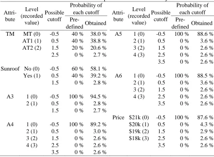
Table 3.4 shows the aggregate estimates of the cutoff probability obtained using the conjunctive model. For discrete attributes, cutoffs are reported in terms of multinomial point mass probabilities. Each level is recorded as an integer (e.g., 0, 1, 2) and the recorded values indicate
l
nim in Eq. (3.2). Thus, a grid of possible cutoff values,
nm, are also specified (e.g.,Table 3.4. Threshold estimates for the posterior means of the conjunctive model Attri-bute Level (recorded value) Possible cutoff Probability of Attri-bute Level (recorded value) Possible cutoff Probability of
each cutoff each cutoff
Pre-
Obtained Pre- Obtained
defined defined
TM MT (0) -0.5 40 % 38.0 % A5 1 (0) -0.5 100 % 88.6 %
AT1 (1) 0.5 40 % 38.8 % 2 (1) 0.5 0 % 3.6 %
AT2 (2) 1.5 20 % 20.6 % 3 (2) 1.5 0 % 2.6 %
2.5 0 % 2.7 % 4 (3) 2.5 0 % 2.6 %
3.5 0 % 2.6 %
Sunroof No (0) -0.5 60 % 58.1 %
Yes (1) 0.5 40 % 39.2 % A6 1 (0) -0.5 100 % 88.5 %
1.5 0 % 2.8 % 2 (1) 0.5 0 % 3.6 %
3 (2) 1.5 0 % 2.6 %
A3 1 (0) -0.5 100 % 94.5 % 4 (3) 2.5 0 % 2.6 %
2 (1) 0.5 0 % 2.8 % 3.5 0 % 2.6 %
1.5 0 % 2.7 %
Price $21k (0) -0.5 100 % 87.6 % A4 1 (0) -0.5 100 % 89.2 % $20k (1) 0.5 0 % 4.3 %
2 (1) 0.5 0 % 3.0 % $19k (2) 1.5 0 % 2.9 %
3 (2) 1.5 0 % 2.6 % $18k (3) 2.5 0 % 2.6 %
4 (3) 2.5 0 % 2.6 % 3.5 0 % 2.6 %
3.5 0 % 2.6 %
The probabilities of each cutoff obtained from the conjunctive model closely correspond with the pre-defined noncompensatory preferences in Table 3.2. For example, 40% of the total respondents were pre-defined to screen out MT in the virtual survey, and the conjunctive model results in 38% doing so. Estimates of cutoff probability equal to approximately 2% reflect the influence of the prior distribution and the inherent noise of MCMC. Therefore, respondents are shown to evaluate attributes 3, 4, 5, and price using a compensatory rule set.