DIFFERENT MULTIPLE INPUT MULTIPLE OUTPUT SYSTEMS

(1)

SYSTEMS

By

Mohammed Alamgir

ID: 3554571

SUBMITTED IN PARTIAL FULFILLMENT OF THE REQUIREMENTS FOR THE DEGREE OF

MASTERS OF ENGINEERING IN ELECTRICAL ENGINEERING AT

VICTORIA UNIVERSITY OF TECHNOLOGY MELBOURNE, AUSTRALIA

MAY 2003

c

(2)

The undersigned hereby certify that they have read and recommend to the Faculty of Engineering and Science for acceptance a thesis entitled “Different Multiple Input Multiple Output Systems” by Mohammed Alamgir in partial fulfillment of the requirements for the degree of Masters of Engineering in Electrical Engineering.

Dated: May 2003

Research Supervisor:

Prof. Mike Faulkner

Research co-supervisor:

Dr. Ying Tan

(3)

Date: May 2003 Author: Mohammed Alamgir

Title: Different Multiple Input Multiple Output Systems Department: School of Communications and Informatics

Degree: M.Eng. Year: 2004

Permission is herewith granted to Victoria University of Technology to circulate and to have copied for non-commercial purposes, at its discretion, the above title upon the request of individuals or institutions.

Signature of Author

THE AUTHOR RESERVES OTHER PUBLICATION RIGHTS, AND NEITHER THE THESIS NOR EXTENSIVE EXTRACTS FROM IT MAY BE PRINTED OR OTHERWISE REPRODUCED WITHOUT THE AUTHOR’S WRITTEN PERMISSION.

THE AUTHOR ATTESTS THAT PERMISSION HAS BEEN OBTAINED FOR THE USE OF ANY COPYRIGHTED MATERIAL APPEARING IN THIS THESIS (OTHER THAN BRIEF EXCERPTS REQUIRING ONLY PROPER ACKNOWLEDGEMENT IN SCHOLARLY WRITING) AND THAT ALL SUCH USE IS CLEARLY ACKNOWLEDGED.

(4)

(5)

Table of Contents v

List of Tables vii

List of Figures ix

Abstract xi

Acknowledgements xiii

1 Overview of the Thesis 1

2 Introduction 4

2.1 Background . . . 5

2.2 Propagation Characteristics of a Radio Channel . . . 6

2.2.1 Attenuation . . . 6

2.2.2 Multipath Effects . . . 7

2.2.3 The Doppler Effect . . . 8

2.2.4 Fading . . . 8

2.2.5 Fading Distributions . . . 9

2.3 Diversity . . . 11

2.4 Adaptive Modulation . . . 13

2.5 Channel Capacity . . . 15

2.5.1 Entropy and Mutual Information . . . 15

2.5.2 Channel Capacity . . . 16

2.6 Multiple Input Multiple Output Scheme . . . 16

(6)

2.10 Measurement of Capacity . . . 22

2.11 Simulation Results . . . 23

3 Bell Labs Space Time Architecture 27 3.1 Introduction . . . 28

3.2 Detection Process . . . 29

3.2.1 Nulling . . . 29

3.2.2 Interference Cancellation . . . 30

3.3 Optimal Detection Order . . . 31

3.4 Computing the ZF Nulling Vector . . . 31

3.5 Computing the MMSE Nulling Vector . . . 32

3.6 Detection Algorithm . . . 32

3.7 Complexity Analysis . . . 33

3.8 QR Decomposition Based Detection . . . 35

3.9 Backward and Forward Sweeps . . . 37

3.10 Optimal Ordering . . . 38

3.11 Complexity Analysis of the QR Decoder . . . 39

3.12.1 BER, BLER and Throughput . . . 40

3.12.2 Execution Time . . . 45

4 New Detection Method for VBLAST 47 4.1 The Polar Decomposition . . . 48

4.2 Detection Using the Cholesky Factorization . . . 48

4.3 Detection Using the QR Factorization . . . 49

4.4 Optimal Ordering . . . 50

4.5 Properties of the Polar Decomposition . . . 50

4.6 Behavior of Q and P Matrices . . . 51

4.7 Algorithms for the Polar Decomposition . . . 51

4.7.1 Higham’s Algorithm for Polar Decomposition . . . 52

4.8 Complexity Analysis . . . 54

(7)

4.9.1 BER, BLER and Throughput . . . 54

5 Singular Value Decomposition Based MIMO Systems 58 5.1 Introduction . . . 59

5.2 SVD Based MIMO Systems . . . 59

5.3 Behavior of U, D and V Matrices . . . 61

5.4 SNR of Parallel Subchannels . . . 62

5.5 Power Control . . . 63

5.6 Adaptive Modulation across Subchannels . . . 64

6 Performance Comparison Results 67 6.1 Introduction . . . 67

6.2 Channel Models . . . 68

6.2.1 IID Channels . . . 68

6.2.2 Slow Fading Rayleigh Channel . . . 69

6.2.3 VUT Measured Channel . . . 69

6.3 Variants of VBLAST . . . 69

6.3.1 BER, BLER and Throughputs . . . 70

6.4 VBLAST System vs SVD-based System . . . 73

6.4.1 IID Channels . . . 75

6.4.2 IID Rank Deficient Channel . . . 78

6.4.3 Slow Fading Rayleigh Channel . . . 79

6.4.4 VUT Measured Channel . . . 80

7 Conclusion and Further Work 86

Bibliography 88

(8)

6.1 Acronyms used to denote different MIMO systems. . . 68 6.2 Complexities of different VBLAST methods. . . 72 6.3 Correlation among the singular values of measured channels. . . 83

(9)

2.1 Typical Rayleigh fading of a signal. . . 10

2.2 PDFs of Rayleigh and Ricean distributions. . . 11

2.3 ES/N0 vs BER for MQAM constellations. . . 14

2.4 MIMO transmission scheme. . . 17

2.5 Mean capacity of different MIMO systems. . . 24

2.6 Capacity CCDFs of different MIMO systems at SNR = 0dB. . . 24

2.7 MIMO capacity CCDF for different SNRs. . . 25

2.8 MIMO mean capacity with waterfilling, (4×4 system). . . 26

3.1 The VBLAST architecture. . . 29

3.2 Bit error rate of the VBLAST system in IID random channel. . . 40

3.3 Block error rate of the VBLAST system in IID random channel. . . 41

3.4 Throughput of the VBLAST system in IID random channel. . . 41

3.5 Bit error rate of the VBLAST system in IID random channel with opti-mal ordering. . . 42

3.6 Bit error rate of QR based VBLAST system in IID random channel. . . 43

3.7 Effect of optimal ordering on bit error rate. . . 43

3.8 Effect of optimal ordering and backward/forward sweep on bit error rate. 44 3.9 Throughput of QR-based VBLAST system. . . 44

3.10 Theoretical complexity of the VBLAST and QR methods. . . 46

3.11 Execution time of the VBLAST and QR methods. . . 46

4.1 Polar Decomposition behavior . . . 52

4.2 Bit error rate of Polar Decomposition-based VBLAST. . . 55

4.3 Block error rate of Polar Decomposition-based VBLAST. . . 56

4.4 Throughput of Polar Decomposition-based VBLAST. . . 56

4.5 Complexity of VBLAST and Polar Decomposition-based VBLAST. . . . 57

(10)

5.1 SVD-based MIMO transmission scheme. . . 60

5.2 SVD-based MIMO transmission in TDD channel (taken from [22]). . . 61

5.3 Changes in U, V and D matrices for a slowly varying channel matrix H. 62 5.4 Bit error rate of the SVD system. . . 65

5.5 Throughput of the SVD system. . . 66

6.1 Floor map of the measurement. Rx is receiver position, A is LOS point and B is NLOS point. . . 70

6.2 Bit error rate of VBLAST for different decoding methods. . . 71

6.3 Bit error rate of different VBLAST decoding methods with optimal decoding order. . . 72

6.4 Theoretical complexity of VBLAST decoding methods. . . 74

6.5 Execution time of VBLAST decoding methods. . . 74

6.6 CPU time of VBLAST decoding methods. . . 75

6.7 Throughput of different MIMO systems. . . 76

6.8 Block error rate of different MIMO systems. . . 77

6.9 Bit error rate of different MIMO systems. . . 77

6.10 Effect of the optimal order and waterfilling. . . 78

6.11 Throughputs of VBLAST-ZF-opt and SVD-adap systems in rank defi-cient IID channel. . . 79

6.12 Bit error rate of VBLAST-ZF-opt and SVD-adapt systems in rank de-ficient IID channel . . . 80

6.13 Throughput of VBLAST-opt system in slow fading Rayleigh channel. . 81

6.14 Throughput of SVD-adapt system in slow fading Rayleigh channel. . . 81

6.15 Singular values of measured channel with LOS path. . . 82

6.16 Singular values of measured channel with NLOS path. . . 82

6.17 Throughputs of VBLAST-ZF-opt and SVD-adapt systems in measured channel. . . 84

6.18 Bit error rates of VBLAST-ZF-opt and SVD-adapt systems in measured channel. . . 84

(11)

The use of multiple antennas at the transmitter as well as at the receiver can greatly improve the capacity of a wireless link when operating in a rich scattering environment. In such an arrangement all transmitting antennas radiate in the same frequency band so the overall spectral efficiency becomes very high. Such a multiple antenna scheme, popularly known as Multiple Input Multiple Output (MIMO) has potential application in wireless local area networks (WLAN) and cellular micro-cells. One reason is that the WLANs and other short range wireless systems often operate in an indoor environment, which offers rich scattering. The other reason is the demand for higher data rates in cellular and WLAN systems to cater for multimedia services. Recently researchers have proposed different architectures for materializing the potential of the MIMO scheme. VBLAST (Vertical-Bell Labs Space Time) is a popular architecture that will play an important role in future standardizations. Furthermore, different decoding methods have been proposed for VBLAST. The SVD (Singular Value Decomposition) based system is envisioned as a highly effective MIMO technique in a TDD (Time Division Duplex) framework. Such a system operates by adapting the constellation size across different subchannels.

In this work we study the VBLAST and SVD architectures and compare the perfor-mance and computing power requirement of these architectures. Also in this study a new efficient decoding method for the VBLAST architecture is proposed. The original VBLAST decoding method relies on the repetitive computation of the pseudoinverse

(12)

of the channel matrix. Alternatively, there are methods based on the QR decomposi-tion, the matrix square root etc. Our new decoding method is based on a relatively less known matrix decomposition, the Polar Decomposition. The new method requires less computation and has several other advantages like the possibility of incremental updates, channel rank tracking, etc. We consider three different types of channels: IID random, slow fading and measured channels. The entire work is simulated in the MATLAB environment.

(13)

I would like to thank my supervisor Professor Mike Faulkner, who first has rescued me from the frustration of doing course work and then continued his support and direction during the course of this research. Without his generous help it would have been impossible to finish this work.

Next comes cosupervisor Ying Tan who has offered his maximum help to get me into MIMO and kept his support continuous. Also thanks for Melvyn Pierra, Guillame Lebrun and Jason Gao at Telecommunication and Microelectronics Center. They have helped me by providing papers, suggestions and in many other ways.

The AusAID has provided the funds for my study and living through a scholarship. AusAID liaison officer, Kerry Wright was my resort in bad times in Melbourne; she deserves special mention.

A heartfelt gratitude for the people of Bangladesh who have supported my un-dergraduate study in Bangladesh. Also thanks to Shahjalal University of Science and Technology, Sylhet, Bangladesh for approving me of Study Leave to pursue this degree. I am grateful to my parents for bringing me into this world and to my siblings for keeping a warm family where I grew up. My wife Geeti has always supported me and deserves more than mere acknowledgement.

Finally, I wish to thank Gavin, Trung, Andrew, Edward and Way Wu for spending a wonderful time in the room D708. The Thursday soccer team is also owed thanks.

Mohammed Alamgir Melbourne, Australia

(14)

Overview of the Thesis

This chapter gives an overview of the contents of this thesis. The chapters of interest are the following:

• Chapter 1 Overview of the thesis

• Chapter 2 Introduction: Chapter two starts by discussing the characteristics of the radio channel such as attenuation, multipath, the Doppler effect and fad-ing. Transmit diversity techniques are introduced and different techniques are discussed briefly. A short paragraph shows how adaptive modulation techniques can counter fading. Information theoretic terms such as entropy, mutual infor-mation and capacity are elaborated. An introduction to the MIMO scheme is given followed by the calculation of the theoretical capacity. Power control issues are discussed. The definitions of outage capacity and system throughput, the practical ways of measuring capacity, are given. Some simulation results are then shown. Most of the concepts presented in this chapter are known.

• Chapter 3 Bell Labs Space Time Architecture: This chapter deals with

(15)

the aspects of the VBLAST architecture. An introduction to the VBLAST ar-chitecture is given followed by its operation. The detection method, nulling, interference cancellation, and optimal ordering are discussed thoroughly. The decoding algorithm is studied, and an exact unreported complexity analysis of the decoding algorithm is done. Then it is shown how the QR decomposition can be used to decode VBLAST signals. Benefits of forward and backward sweeps are considered, including ordering for optimal detection. A calculation of complexity follows. The chapter ends with some simulation results showing the performances of the original VBLAST and the QR method.

• Chapter 4 New Detection Method for VBLAST: One of the two major contributions of the present work and this thesis is in this chapter. The chapter introduces a new detection method for the VBLAST system using a relatively less known matrix decomposition, the Polar Decomposition (PD). The Polar Decomposition is introduced and Cholesky and QR factorizations are used to decode the VBLAST signals. The issue of optimal ordering is also discussed. The properties of the PD are discussed, and then it is shown how these properties are conducive to the VBLAST detection. Algorithms for the PD are reviewed with complexity analysis. The chapter ends with some simulation results and comments.

(16)

chapter introduces the Singular Value Decomposition (SVD)-based MIMO sys-tem. Such systems are suitable for Time Division Duplex (TDD) mode of com-munication and can get very close to the theoretical capacity limit. The detailed architecture and properties of the SVD system are discussed. The SVD produces parallel subchannels of different gains and adaptive modulation is used across them. Power control issues are also addressed. The chapter concludes with some simulation results and comments.

• Chapter 6 Performance Comparison Results: This chapter contains the re-sults of the simulations performed under different conditions. Three types of channel models are considered. They are: the IID (independently and identically distributed) random channel, a slow fading Rayleigh channel and a physical chan-nel measured by the VUT MIMO group. The BER performance and execution time of the different decoding methods for VBLAST are reported. A comparison between VBLAST and SVD systems is also performed.

(17)

Introduction

Chapter Outline

This chapter starts by discussing the characteristics of radio channels such as atten-uation, multipath, the Doppler effect and fading (section 2.2). Transmit diversity techniques are introduced in section 2.3, and then section 2.4 shows how adaptive modulation techniques can counter the fading. Information theoretic terms such as entropy, mutual information and capacity are elaborated in section 2.5. Section 2.6 introduces the MIMO scheme followed by a calculation of the theoretical capacity of the MIMO channel. The definitions of outage capacity and system throughput, the practical ways of measuring capacity, are given in sections 2.9 and 2.10 respectively. Some simulation results are then shown in section 2.11. The chapter ends making a few comments. Most of the concepts presented in this chapter are classical.

(18)

2.1 Background

Wireless devices such as mobile phones have been gaining more and more popularity mainly because of their mobility. Though voice was the only service available on early phones, text service has now been added, and more recently multimedia services, such as pictures and videos have started to emerge. These services are not widespread, but the demand for them is on the rise. At the same time wireless local area networks (WLAN) still have to compete with their wireline counterparts mainly because of their high data rates. Wireless local area networks are attractive for their mobility, but the high data rates available on the wireline network still seem to be unreachable in wireless networks. A requirement for high data rates directly translates into a wider bandwidth requirement which is not feasible because of the limited radio spectrum. Nevertheless, digital wireless systems are slowly replacing ordinary analog ones. Examples include the new standards for radio and television broadcast, the digital audio broadcasting, DAB and digital video broadcasting, DVB.

(19)

the Shannon limit. Data transmission at rates higher than the Shannon limit have never been thought possible until very recently.

2.2 Propagation Characteristics of a Radio Channel

In a real environment radio waves from mobile devices travel through the air, build-ings and other obstacles. Reflections from different objects cause the waves to travel through multiple paths to the receiver. The movement of objects in the channel or that of the receiver cause an apparent shift in the carrier frequency. A reliable commu-nication system tries to overcome or take advantage of these channel perturbations.

2.2.1 Attenuation

Attenuation is the loss of average received signal power. Factors responsible for atten-uation are the distance between the transmitter and receiver, the obstacles in between, their physical properties, etc. Attenuation due to distance increases exponentially, and, in addition to this, the presence of very large obstacles such as buildings, hills, etc causes another type of attenuation known as log normal shadowing. Geometric models have been proposed to explain these large scale power losses but statistical models are often used because of their accurate description of particular real environments. Statistically, the attenuation is considered as a random variable having a well known distribution. A common formula used to model attenuation is

P L(d)[dB] =P L(d0) + 10nlog

d d0

(20)

where, Xσ is a zero mean Gaussian distributed random variable (in dB) with standard

deviation σ (also in dB) and accounts for the log normal shadowing effect. The path loss at any arbitrary distancedis statistically described relative to the close-in reference pointd0, the path loss exponent n, and the standard deviationσ. The exponentncan

have values from 1.6 (in indoor line of sight) up to 6 (in highly builtup cites).

2.2.2 Multipath Effects

Radio waves traveling along different paths arrive at the receiver at different times with random phases and combine constructively or destructively. The net result is a rapid fluctuation in the amplitude of the received signal in a short period of time or distance travelled. However, the large scale average path loss remains constant. Multipath propagation had previously been considered a problem, but now it is exploited to achieve higher capacity.

The multipath structure of a channel is quantified by its delay spread or by its root-mean-square (RMS) value. A channel having delay spread less than the symbol period of transmission offers frequency nonselective attenuation, and a larger value of delay spread means there is frequency selective variation in the channel. Another parameter, the coherence bandwidth is also often used to describe the frequency se-lectiveness and is related to the delay spread as

Bc ≈

1 50στ

(2.2.2)

(21)

2.2.3 The Doppler Effect

When there is relative movement between the transmitter and receiver, the carrier frequency, as perceived by the receiver, gets changed by some amount; this is known as the Doppler effect. The amount of frequency shift depends on the relative speed, the direction of movement and the frequency of the carrier. In mathematical terms

fd=

v

λ ×cosθ (2.2.3)

where v is the relative speed between the transmitter and receiver, θ is the angle between the direction of motion and the wave propagation, and λ is the carrier wave-length. A Doppler shift can be negative as well as positive, meaning an apparent decrease or increase in frequency, respectively. However, most often the maximum ab-solute value is considered and normalized with respect to the symbol rate and denoted by FdT

FdT =

|fd|

fsymbol

(2.2.4)

where fsymbol is the symbol rate. A typical office environment hasFdT value of about

2−3

. Another parameter, often used to characterize the time varying nature of the channels is the coherence time which is related to the Doppler shift by

Tc ≈

9 16πfm

(2.2.5)

where fm is the maximum Doppler shift given by fm =v/λ [23].

2.2.4 Fading

(22)

is constant. A fade can be flat or frequency selective depending on the multipath structure of the channel, and slow or fast depending on the Doppler effect. Flat fading occurs when the bandwidth of the signal is less than the coherence bandwidth. This type of fading is common, and some communication systems are designed specifically to operate in very narrow bandwidth mode. If the signal bandwidth is wider than the coherence bandwidth then different frequencies undergo independent fading and the result is inter-symbol-interference (ISI).

How rapidly the channel changes as compared to the signal variation determines whether the fading is slow or fast. The Doppler effect is the reason for this type of fading as any movement of the receiver or any object in the channel produces a Doppler shift. The symbol period of the transmitted signal has to be shorter than the coherence time for a slow fading channel.

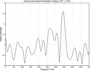
A channel can be either flat or frequency selective and either slow or fast fading. A typical office environment is slow fading. New techniques (such as OFDM) are designed to use very low bandwidth subchannels so that the fading can be regarded flat. Fig. 2.1 shows typical fading for a signal with an FdT value of 0.02.

2.2.5 Fading Distributions

(23)

0 50 100 150 200 250 300 350 400 450 500 0 0.5 1 1.5 2 2.5 3 Elapsed Time Signal Strength

Typical Simulated Rayleigh Fading, FdT = 0.02

Figure 2.1: Typical Rayleigh fading of a signal.

of a Rayleigh distribution is given by

p(r) =   

r σ2 exp

−r2 2σ2

(0≤r ≤ ∞)

0 (r <0) (2.2.6)

where σ is the RMS (amplitude) value of the received signal and σ2

is the average power. In an indoor environment where the chance of a line of sight path is high, the fading follows a Ricean distribution with PDF

p(r) =   

r σ2 exp

−(r2+A2₎ 2σ2 I0

Ar σ2

(A≥0, r≥0)

0 (r <0) (2.2.7)

where A is the peak amplitude of the dominant path and I0(.) is the modified Bessel

(24)

0 0.1 0.2 0.3 0.4 0.5 0.6 0.7 0.8 0.9 1 0

0.02 0.04 0.06 0.08 0.1 0.12 0.14 0.16

Received Signal Strength

p(r)

PDFs of Rayleigh and Ricean Distributions

Rayleigh Ricean

Figure 2.2: PDFs of Rayleigh and Ricean distributions.

2.3 Diversity

In a scattering environment the individual signal path arriving at the receiver faces independent or highly uncorrelated fading. This means that when a particular signal path is in a fade there may be another signal path not in any fade. The receiver can exploit this fact by receiving more than one path and choosing and/or combining them. Widely used schemes to do this are: selection diversity where the path with the best average signal to noise ratio (SNR) is chosen, equal gain combining where the different paths are cophased and added together and MMSE combining where the different paths are weighted and then added (weighting coefficients are chosen during a training phase). Receiver diversity can improve the average SNR by 20dB to 30dB.

(25)

• Space Diversity: Also known as antenna diversity, space diversity uses more than one antenna at the receiver. The signals received on antennas separated by a half wavelength or more tend to be decorrelated [2]. This is because in a rich scattering environment the chance of a line of sight path is low, and most paths are reflected or diffracted from obstacles. Usually antenna diversity is used only at the base station because multiple antennas on the portable unit pose a design challenge and do not justify the cost.

• Polarization Diversity: Electromagnetic waves have vertical and horizontal po-larizations that also show decorrelation [3]. Where the required antenna spacing for space diversity is not feasible, polarization diversity is used as an alternative as the same antenna can be used for different polarizations. However, it is not possible to have more than 2-way polarization diversity.

• Frequency Diversity: Frequencies separated by more than the coherence band-width of the channel suffer independent fades. Frequency diversity takes advan-tage of this fact by transmitting at more than one carrier frequency. The GSM standard uses frequency hopping to achieve frequency diversity.

• Time Diversity: In time diversity the same information symbol is repeatedly transmitted at different time slots with the hope that they will suffer independent fading and the receiver will combine them properly. While highly effective in fast fading environments, time diversity is not as effective in slow fading channels unless a large decoding delay can be tolerated. A coding structure known as

(26)

code before any transmission takes place.

2.4 Adaptive Modulation

Traditional communication systems use fixed constellations among which QPSK and MQAM are popular. A QPSK constellation uses two quadrature carriers each of which is BPSK modulated. In MQAM the phase as well as the amplitudes of a pair of quadra-ture carriers are varied according to the binary data. Whereas QPSK can transmit a maximum two bits per symbol, MQAM can send log2M bits per symbol. However,

higher level constellations have higher probabilities of error thus requiring higher SNRs to achieve a given bit error rate (BER). The symbol error rate (SER) of an MQAM constellation with ideal detection is bounded by [4]

PS ≤ 1−

"

1−2Q

s

3ES

(M −1)/N0

!#2

(2.4.1)

where ES is the average symbol energy, N0 is the Gaussian noise power, M is the

constellation size and Q(.) is the Q-function. The BER is related to the SER by

PB =

2k₋1

2k₋₁PS (2.4.2)

where k= log2M. A plot of BER vs Es/N0 for different M is shown in Fig. 2.3.

(27)

0 5 10 15 20 25 30 35 10−7

10−6 10−5 10−4 10−3 10−2 10−1

E_S/N₀

BER

SNR vs BER

QPSK 8QAM 16QAM 32QAM 64QAM

Figure 2.3: ES/N0 vs BER for MQAM constellations.

(TDD) scheme both ends of the communication link have knowledge of the channel, and so they can adapt the constellation size without extra feedback. To make a decision about the size of the constellation, the average available SNR (which signifies the channel condition) and maximum acceptable target BER should be given. In some applications (such as speech) the overall throughput is important and bit errors are not critical, while in other applications (like file transfers) a very low BER is more important than the throughput.

In an ideal situation, a continuous adaptation of the constellation is required but in practice one can have only integer constellation sizes. Constellation sizes of 2k

i.e, 2, 4, 8, 16, 32, etc are used commonly. In [5] it was shown that even such a discrete adaptation can closely approximate the ideal case. In this work we use only square constellations such as QPSK, 16QAM and 64QAM. Also 10−6

(28)

acceptable BER and hence lower bounds the minimum SNR required for each of these constellations. Fig. 2.3 implies that if the available SNR is 27dB or more 64QAM should be used; if the SNR degrades to between 21dB and 24dB, 16QAM should be used. If the SNR is between 13dB and 17.5dB QPSK should be used. At an SNR less than 13dB transmission would stop.

2.5 Channel Capacity

2.5.1 Entropy and Mutual Information

The entropy of a discrete random variable X is defined as [6]

H(X) =−

n

X

j=1

pjlog2(pj) (2.5.1)

where pj is the probability thatX=j. Entropy measures the uncertainty of a random

variable, and so, it is an indication of the information contained in that variable [6]. Based on the joint probability, thejoint entropy of two random variablesX, Y is defined to be

H(X, Y) =−

n

X

j=1 m

X

k=1

pjklog2(pjk) (2.5.2)

where pjk is the joint probability that X =j and Y =k. If X and Y are dependent

and pj(k) denotes the conditional probability that Y = k given X = j, then the

conditional entropy of Y givenX, denoted by H(Y|X) is defined as

H(Y|X) =−

n

X

j=1 m

X

k=1

pjklog2(pj(k)) (2.5.3)

The mutual information of two random variables, X and Y, denoted as I(X;Y) is given by

(29)

For any two random variables X and Y, I(X;Y) = I(Y;X). Also I(X;Y) = 0 when X and Y are independent.

2.5.2 Channel Capacity

Shannon [1] defines the capacity of a channel as the maximum data rate at which data transmitted from a transmitter, when passed through the channel, can be received at some receiver with negligible chance of error. If the data source and received data are viewed as random variables, then the channel capacity refers to the maximum mutual information between them. The capacity C is

C= max

p(x) I

(X;Y) (2.5.5)

where the maximization is taken over all possible probability distributionsp(x)ofX. A data source with Gaussian probability distribution has the maximum entropy. Thus, to achieve a data rate close to the capacity, the data source should be Gaussian distributed. For a bandlimited channel with noise being Gaussian and white, Shannon [1] derived the normalized capacity (capacity per unit bandwidth) to be

C = log2(1 +ρ) bps/Hz (2.5.6)

where ρ is the received SNR.

2.6 Multiple Input Multiple Output Scheme

(30)

x y

Tx Rx

H

Figure 2.4: MIMO transmission scheme.

band. By sharing the same frequency band the spectral efficiency becomes very high. The receiver is assumed to have ideal channel estimates so it can separate and decode the symbols transmitted from each antenna. The ability to separate out the symbols is due to the fact that in a scattering environment, the signals received at each receiving antenna from each transmitting antenna appear to be uncorrelated. Fig.2.4 shows a block diagram of such a scheme.

2.7 Capacity of MIMO Systems

A baseband MIMO system with t transmit antennas and r receive antennas can be modelled by the linear relationship

y=Hx+n (2.7.1)

(31)

between the jth transmit antenna and ith receive antenna. With hij being complex

Gaussian, the magnitude |hij| is Rayleigh distributed. In a rich scattering environment

the columns of H are assumed to be independent. The mutual information is then

I(x;y) = H(y)− H(y|x)

= H(y)− H((Hx+n)|x)

= H(y)− H(n|x)

= H(y)− H(n) (2.7.2)

where the transmit vectorxand noise vectornare assumed independent of each other. The third equality holds because H is constant (zero entropy) during the transmission of a whole block of x. Eq. (2.7.2) is maximized when yhas the maximum entropy of log2det(πeK). This requires y to be a circularly symmetric complex Gaussian vector

with covariance matrixE{yy′}=K [7] where′_{denotes complex conjugate transpose.} If the transmit vector xis also complex Gaussian vector with covarianceE{xx′}=Q, then K can be found by

K = E

(Hx+n) (Hx+n)′

= E{Hxx′H′}+E{nn′}

= HQH′₊_Kn

= Ks

+Kn

(2.7.3)

where the fact thatxand nare independent and zero mean is used. Here Ks

and Kn

(32)

maximum mutual information, which is also the capacity, is

C = H(y)− H(n)

= log2[det (πe(K s

+Kn))]−log2[det (πeK n

)]

= log2

det (Ks

+Kn

) (Kn

)−1

= log2

det Ks(Kn)−1

+Ir

= log2

det HQH′(Kn)−1+Ir

(2.7.4)

where Ir is the r×r identity matrix. The noise received at each receiving antenna

is assumed to be uncorrelated so, Kn

= σ2

Ir, σ 2

being the noise power on each receiving antenna. Also, when the transmitter has no knowledge about the channel, it is optimum to use equal power on each antenna [7]; that means Q = Pt

t It, Pt being

the total signal power. The MIMO channel capacity then becomes

C = log2

h det

Ir+

ρ tHH

′i _(2.7.5)

where Pt/σ 2

has been replaced by ρ, the average SNR at each receiving antenna.

2.8 Power Control

According to the singular value theorem [16], any matrixH ∈Cr×t

can be decomposed as

H =UDV′ (2.8.1)

where U ∈ Cr×r

and V ∈ Ct×t

are unitary and D ∈ Rr×t

(33)

HH′_{. Thus, (2.7.1) can be written as}

y=UDV′x+n. (2.8.2)

Letting y˜ =U′_y_,_x_˜ ₌_V′_x_and _n_˜ ₌_U′_n _{(2.8.2) becomes}

˜

y=Dx˜+ ˜n. (2.8.3)

As U and V are unitary, the distributions of y˜, x˜ and n˜ are respectively the same as those of y, x and n. The original channel H is now equivalent to a set of parallel channels whose gains are the diagonal entries of D. Since the rank of H is limited to min{r, t}, only min{r, t} diagonal elements of D are nonzero. Denoting them by λi,

the parallel subchannels are

˜

yi =λix˜i+ ˜ni 1≤i≤min{r, t} (2.8.4)

Telatar [7] showed that the optimum (giving maximum channel capacity) power of the

ith subchannel is µ− 1 λ2

i

+

where the parameter µ is determined by the total power

Pt such that

Pt=

X

i

µ− 1

λ2 i

+

. (2.8.5)

The notation a+

denotes max{0, a}. With this optimum power control, the channel capacity becomes

CW F =

X

i

log2 µλ 2 i

+

. (2.8.6)

Rewriting this in the form of (2.7.5), the capacity is

CW F = log2

det

Ir+

1

σ2HQH˜

′

(34)

where Q˜ii =

µ− 1 λ2

i

. Also we have Q˜ = UQU′_{, that implies} _Q ₌ _U′_QU˜ _{, the} transmit covariance matrix of the original system of (2.7.1).

Finding the value of parameterµfrom (2.8.5) involves a fair amount of compu-tation. Moreover, if the transmitter’s estimation ofH is incorrect (and thus the values

λi), then waterfilling can give a worse capacity than the equal power rule. The effect

of incorrect channel estimation on waterfilling and capacity has been studied in [8].

2.9 Outage Capacity

The capacity described by (2.7.5) or (2.8.7) is instantaneous, for a given realization of channel H. Since in Rayleigh fading the channel matrix H changes randomly, the capacity is also random. One way to express the capacity of a such a channel is the ergodic mean of (2.7.5) or (2.8.7). However, this mean capacity is not very useful in termes of the outage capacity. Outage capacity is related to the outage probability, which is the fraction of time the capacity falls below a given threshold Coutage. The

outage probability q is defined as

q =Pr{C ≤Coutage} (2.9.1)

This can also be expressed as

1−q=Pr{C > Coutage} (2.9.2)

(35)

2.10 Measurement of Capacity

The theoretical capacities as discussed above are the absolute limit under all ideal conditions. However, a real system can only achieve a portion of that capacity. The throughput of a real system is defined as a parallel quantity to express the spectral efficiency of a given system. Here, capacity refers to the absolute achievable limit with the particular system architecture.

A communication system employing MQAM constellations with ideal Nyquist pulses (Sinc[t/Ts]), occupies a bandwith of W = 1/Ts and supports a bit rate of

R = (log2M)/Ts. For such an uncoded MQAM system, the throughput, in bps/Hz

is log2M. However, there are errors, and if the transmission is in form of blocks of

L bits, then the effective throughput in terms of the block error rate (BLER) can be written as [10]

T = (log2M)×(1−BER)

= (log2M)×

1−(1−BER)L. (2.10.1)

Here, BER is the bit error rate of the data stream. For a MIMO syste there is more than one substream of data, each of which has a throughput of (2.10.1). The total throughput of the system is then

Ttot = n

X

i=1

Ti (2.10.2)

(36)

2.11 Simulation Results

This section shows some plots derived from (2.7.5) and (2.8.7) for different SNRs and (r, t) pairs. The outage capacity as discussed in section 2.9 can also be expressed in terms of its cumulative distribution function (CDF). However, its complementary cumulative distribution function (CCDF) is more often used. As an exact closed form expression of the CDF or CCDF is highly involved, this section shows numerically derived capacities of CCDs obtained from Monte-Carlo simulated data.

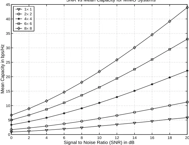
Fig. 2.5 shows the mean capacity of MIMO systems as a function of SNR for different (r, t) combinations. The (1,1) system capacity is equivalent to the SISO Shannon capacity but for a Rayleigh channel. At high SNR, for a (1,1) system the increase in capacity is roughly 1 bit for a 3dB increase in SNR. However, in MIMO, even for a (4,4)system, a 3dB increase in SNR results in about 4 bits of increase in capacity. The capacity increase is almost linear in terms of (r, t), for r=t.

The capacity CCDFs are shown in Fig. 2.6 for a system with 0dB SNR. We can see, for example, that for a (4,4)system the capacity is about 2.5bps/Hz with 5% outage probability. For a (8,8)system this is about 5.8 bps/Hz.

The capacity CCDF as a function of SNR is shown in Fig. 2.7. Only (1,1)and (4,4) systems are depicted for comparison. We see that at a 5% outage probability level the capacity increase is about 2bps/Hz for every 3dB increase in SNR whereas for the (1,1)case the increase is not even visible at low SNRs and is only a fraction of a bit at high SNRs.

(37)

0 2 4 6 8 10 12 14 16 18 20 0

5 10 15 20 25 30 35 40 45

Signal to Noise Ratio (SNR) in dB

Mean Capacity in bps/Hz

SNR vs Mean Capacity for MIMO Systems

1× 1 2× 2 4× 4 6× 6 8× 8

Figure 2.5: Mean capacity of different MIMO systems.

0 1 2 3 4 5 6 7 8 9 10

0 0.1 0.2 0.3 0.4 0.5 0.6 0.7 0.8 0.9 1

Capacity in bps/Hz

Prob(Capacity > Abscissa)

CCDF of MIMO Capacity, SNR=0dB

1× 1 2× 2 4× 4 6× 6 8× 8 5%Outage Level

Left to right

(38)

0 5 10 15 20 25 30 0.5

0.55 0.6 0.65 0.7 0.75 0.8 0.85 0.9 0.95 1

Capacity in bps/Hz

Prob(Capacity > Abscissa)

CCDF of MIMO Capacity for different SNRs

SNRs: Left to right 0, 3, 6, 9, 12, 15 18, 21 dB

4x4 system

1x1 system

Figure 2.7: MIMO capacity CCDF for different SNRs.

reported by [9], waterfilling is only effective at very low SNRs. For high SNRs power control does not improve the capacity as much as it does for low SNRs.

(39)

−100 −8 −6 −4 −2 0 2 4 6 8 10 2

4 6 8 10 12 14 16 18

Signal to Noise Ratio (SNR) in dB

Mean Capacity in bps/Hz

Waterfilling Capacity

Waterfilling Equal Power

(40)

Bell Labs Space Time Architecture

Chapter Outline

This chapter deals with aspects of the VBLAST architecture. Section 3.1 introduces the VBLAST architecture and its operation. The detection method, nulling, interference cancellation and optimal ordering are discussed in sections 3.2 and 3.3. The decoding algorithm is given in section 3.6, and an exact unreported complexity analysis of the decoding algorithm is done in section 3.7. This is one of the contributions of this thesis. Section 3.8 shows VBLAST decoding using the QR decomposition. The benefits of forward and backward sweeps are considered in section 3.9, including ordering for optimal detection in section 3.10. Calculation of complexity are given in section 3.11. The chapter ends with some simulation results showing the performance of the original VBLAST and QR methods.

(41)

3.1 Introduction

(42)

QAM

QAM QAM

QAM

Serial

Parallel to

Binary Data Channel

MIMO

Processing VBLAST

Binary Data

Receivers Transmitters

Figure 3.1: The VBLAST architecture.

3.2 Detection Process

The detection process of the VBLAST system involves is the estimation of x given y

and H in

y=Hx+n. (3.2.1)

The t elements of the transmit vector xare constellation symbols which are assumed to be uncorrelated. We also assume that the channel matrixH is full rank. It is shown later that the second assumption is very crucial to the operation of the VBLAST system. The receiver knows the received vector y and has an estimation of H. The detection process is then a multiuser detection type process. The process involves two steps [13]:

• Slicing (and then decoding) a symbol while nulling the others

• Cancelling the effect of each new decoded symbol from the rest

3.2.1 Nulling

Denoting the ith column of H as hi the received vector can be written as

(43)

here xi is the transmitted symbol from the ith transmit antenna. Nulling is performed

by linearly weighting the received symbols to satisfy the zero forcing (ZF) orminimum mean squared error (MMSE) performance criterion. The zero forcing nulling vector

wi is chosen such that

wiThj =

(

0 for i6=j

1 for i=j (3.2.3)

where ()T

indicates transpose. Then, the decision statistic for the ith symbol is

di = w T i y

= x1w T

i h1+x2w T

i h2+· · ·xiwTi hi· · ·+xtwTi ht+wTi n

= 0 + 0 +· · ·+xi+· · ·+ 0 + ˜ni

(3.2.4)

A soft or hard decision now can be made ondi to estimate the the transmitted symbol

ˆ

xi =Q(di) (3.2.5)

where Q(.) is the soft/hard decision function.

3.2.2 Interference Cancellation

The effect of symbols already detected can be subtracted from the symbols yet to be detected. This improves the overall performance when the order of detection is chosen carefully.

Denoting the received vector y by y1, if the nulling vector is w1, then the

decision statistic for the ’first’ symbol is

d1 =w T

1y1 (3.2.6)

Ifxˆ1 =Q(d1)is the estimatedx1 after the decision (soft or hard), then the interference

due to xˆ1 on the other symbols can be subtracted by taking

(44)

assumingxˆ1 =x1, i.e, the decision taken was correct. The next symbol is then detected

by finding w2 and then making a decision on w T

2y2 and so on. The performance of

this successive cancellation and detection scheme depends on the decision taken on each stage, as any wrong decision is propagated through all the later stages.

3.3 Optimal Detection Order

To minimize error propagation the ’strongest’ symbols are detected first. This is known to be the optimal detection order.

A simple ‘optimal’ ordering is based on the postdetection SNR of each sub-stream. The SNR for the ith detected symbol of vector y is given by [13]

ρi =

E{|xi|2}

σ2

(||wi||2)

(3.3.1)

where σ2

is the noise power and E{} denotes the expectation. As ||wT i hi||

2

=

||wi||2||hi||2, from (3.2.3) it is seen that a smaller ||wi||2 value requires the

corre-sponding hi have higher 2-norm. So the SNR in (3.2.7) for the ith substream is

proportional to the norm of the ith column of H. Thus, the optimal detection order is in decreasing order of the 2-norm of the columns of H.

3.4 Computing the ZF Nulling Vector

The vector wi in (3.2.3) is unique and is the ith row of the pseudoinverse of H [13]

wTi =

H+

i (3.4.1)

where <>i denotes the ith row and +

(45)

With the successive cancellation and decoding, wiT is chosen as the ith row

of pseudoinverse of H whose 1 to i−1 columns are set to zero. This is due to the fact that at the ith stage the vector wi has to be orthogonal only tohj forj =i tot.

With optimal ordering, if {k1, k2,· · ·kt} denotes the optimal order, at the kith stage

the ZF nulling vector wki is

wTki =

D

H+ ki₋₁

E

ki

(3.4.2)

whereHki₋₁ denotes the matrix obtained fromHby zeroing the columnsk1, k2,· · ·, ki−1.

3.5 Computing the MMSE Nulling Vector

Using the MMSE criterion, the nulling vector wiT is the ith row of the matrix

G=

H′_H₊ 1

ρI

−1

H′ _(3.5.1)

whereρis the SNR [14]. For successive decoding and optimal ordering based onG, the matrix G should be computed on each step from the partially zeroed H as in (3.4.2). The MMSE criterion always results in better SNR and thus a better perfor-mance. But the disadvantages are that the SNR has to be known at the receiver and a matrix inverse needs to be computed.

3.6 Detection Algorithm

The full detection algorithm for ZF VBLAST can be described as follows [13]:

• initialization

(46)

2. G1 =H +

3. k1 = minj|| hG1i_j|| 2

• iteration

1. wT

ki =hGiiki

2. dki =w

T kiyi

3. xˆki =Q(dki)

4. yi+1 =yi−xˆkiHki

5. Gi+1 =H +

ki

6. ki+1 = minj /_∈{k₁,k₂_···ki}|| hGi+1ij|| 2

7. i←i+ 1

Please note that in step 3 (and 6)minj|| hG1i_j|| 2

is used to pick the strongest symbol. This is the due to the reason that the row j of G, which has the minimum 2-norm, corresponds to the j-th column of H which will have the maximum 2-norm.

3.7 Complexity Analysis

(47)

• The complexity of performing the SVD of H =UΣV′ ₍_H _is ₍_r_×_t_{)), using the} R-SVD algorithm is 4r2

t+ 22t3

.

• Computing the pseudoinverse G = H+

= VΣ−1

U′ _needs _r2

t +t2

complex operations. Because the inverse of the diagonal matrix D can be done merely in min(r, t) operations, so it can be ignored. The first matrix multiplication requires only t2

operations because D−1

is diagonal. The second multiplication requires r2

t operations with no need to calculate the transpose. In computing the pseudoinverse, the zero (if any) singular values are left untouched.

So a total of5r2

t+22t3

+t2

complex operations are required to compute the pseudoin-verse. Now, steps (5) and (6) are repeated fori= 1tot. That means the pseudoinverse is computed for deflatedH with decreasing dimensions(r×(t−k)), k = 0,1,2...t−1. The total complex operations count is

t

X

i=1

5r2

i+ 22i3

+t2

which after simplification becomes

8a4

+83 6 a 3 +13 2 a 2 (3.7.1)

under the assumption that r = t = a and consideration of only square or higher exponent terms.

(48)

matrix multiplication requirest2

r, the matrix addition requirest2

and the matrix inverse needs 4t3

(using Gaussian Elimination) operations. The second matrix multiplication takes t3

operations. So the operations count for (3.5.1) is 5t3

+t2

r+t2

. Like before, steps (5) and (6) are repeated fort times with deflatedH. The total operations count is then

t

X

i=1

5i3

+i2

r+i2

.

Taking the square and higher order terms only and setting r =t=a, this becomes

19 12a

4

+19 6 a

3

+23 12a

2

. (3.7.2)

As a matrix inversion costs less than a pseudoinverse, the MMSE criterion requires less computation time than the ZF criterion.

Finding the optimal decoding order (step 6) can use the results of step 5 and does not require computing the pseudoinverse or inverse again. Thus, the complexity of the nulling vector and optimal ordering computation grows as a fourth power of the number of antennas.

3.8 QR Decomposition Based Detection

(49)

r =t =a. The channel matrix H can be QR decomposed:

H =QR (3.8.1)

where Qis a unitary and R is an upper triangular matrix. Then from (3.2.1)

˜

y = Q′_y

= Q′_H_x₊_Q′_n

= Q′(QR)x+Q′n

= Rx+ ˜n. (3.8.2)

In explicit matrix form           ˜ y1 ˜ y2 ˜ y3 .. . ˜ ya           =          

r11 r12 · · · r1a

0 r22 · · · r2a

0 0 · · · r3a

..

. ... ... ... 0 0 · · · raa

                    x1 x2 x3 .. . xa           +           ˜ n1 ˜ n2 ˜ n3 .. . ˜ na           . (3.8.3)

Then the ath received symbol is

˜

ya =raaxa+ ˜na. (3.8.4)

Hence the ath decision statistic da is

da=

1

raa

˜

ya =xa+

1

raa

˜

na. (3.8.5)

Once a decision (hard or soft) is made onda, it is assumed that the estimatexˆa of the

actual transmitted symbolxa is correct, and thus its effect can be subtracted from yet

to be detected symbols. The da−1th decision statistic is then (assuming xˆa =xa)

da₋1 =

1

ra−1,a−1

(ra₋1,a₋1xa₋1+ ˜na₋1+ra₋1,axa−ra₋1,axˆa)

= xa₋1 +

1

ra−1,a−1

˜

(50)

In general the ith decision statistic is

di =

1

rii

yi− a

X

j=i+1

rijxˆi

!

= xi+

1

rii

˜

ni. (3.8.7)

As the symbols are detected successively, any wrong decision will affect the subsequent decisions.

3.9 Backward and Forward Sweeps

To improve the overall performance, Damen et al, [15] have proposed a two-sweep de-tection scheme where the symbols are detected twice, once by backward substitution as shown in the previous section and then again by forward substitution. Then for a given symbol among the two estimates, the ’better’ one is chosen or both are averaged. For a Forward sweep, the channel matrix H is decomposed into, using QL decomposition

H =QfL (3.9.1)

where Qf is unitary (usually different fromQ)and Lis now a lower triangular matrix.

Following a similar approach to (3.8.2) the received vector is

˜

y=Lx+ ˜n. (3.9.2)

In matrix form           ˜ y1 ˜ y2 ˜ y3 ... ˜ ya           =          

l11 0 · · · 0

l21 l22 · · · 0

l31 l32 · · · 0

... ... ... ...

la1 la2 · · · laa

(51)

The first received symbol is

˜

y1 =l11x1+ ˜n1. (3.9.4)

Hence, the first decision statistic d1 is

d1 =

1

l11

y1 =x1+

1

l11

˜

n1. (3.9.5)

The transmitted symbol x1 is then estimated asxˆ1 fromd1. Once again, it is assumed

that the estimatexˆ1 is correct. The next decision statistic is then (assuming xˆ1 =x1)

d2 =

1

l22

(l22x2+ ˜n2+l21x1 −l21xˆ1)

= x2+

1

l22

˜

n2. (3.9.6)

In general the ith decision statistic is

di =

1

lii

yi− i−1

X

j=1

lijxˆi

!

= xi+

1

lii

˜

ni. (3.9.7)

3.10 Optimal Ordering

Similar to the VBLAST optimal ordering, the optimal way of detecting symbols is in the order of decreasing SNR. In (3.8.2) and (3.9.2) the SNR contribution of the symbol

xi to the received signal is

||Ri||

2E{|xi| 2

}

σ2 =||Li||

2E{|xi| 2

}

σ2 =||Hi||

2E{|xi| 2

}

σ2 (3.10.1)

where Hi,Ri and Li are respectively the ith columns of H,R and L and the notation

||.||2

means the 2-norm [15]. Hereσ2

is the noise power. E{|xi| 2

(52)

So in the case of a backward sweep the columns of R should be arranged in increasing order of norm and in the forward sweep the columns ofLshould be arranged in decreasing order of norm. The ordering of columns ofR and L can be done by first permuting the columns of H and then computing the QR decomposition.

3.11 Complexity Analysis of the QR Decoder

As pointed out in [15], in QR decoding most of the time is spent finding the QR factors of the channel matrix. In this study, the Householder method for QR and QL decomposition has been implemented. For a ×a matrix, the Householder method requires 4

3a 3

complex operations to find R or L and an extra 4 3a

3

to getQ [16]. So, a total of 8

3a 3

operations are required for the whole decomposition. To filter the received vector through Q′ _{demands an extra} _a2

operations. Thus the QR method requires

8 3a

3

+a2

complex operations. For the backward and forward sweeps (QR+QL), twice that number of complex operations 16

3 a 3

+ 2a2

are needed. The back substitution is not considered here because the VBLAST system also has a similar step which was not considered in finding the complexity of the VBLAST system.

3.12 Simulation Results

(53)

8 10 12 14 16 18 20 10−4

10−3 10−2 10−1 100

SNR in dB

Bit Error Rate

Bit Error Rate for the VBLAST System, 4x4, IID Channel QPSK−ZF QPSK−MMSE 16QAM−ZF 16QAM−MMSE 64QAM−ZF 64QAM−MMSE

Figure 3.2: Bit error rate of the VBLAST system in IID random channel.

3.12.1 BER, BLER and Throughput

Fig. 3.2 shows the BER performance of VBLAST using different constellation sizes. Both the ZF and MMSE criteria are used. The channel model is IID random. It is well known that larger constellation sizes require comparatively higher SNRs for a given BER. We see that 64QAM has the highest BER and QPSK the lowest in Fig. 3.2. Fig. 3.3 shows the probability of a block error. It should be recalled that a block is in error when one or more bits are in error as no form of coding is used. For 64QAM the block error rate is so high that almost every block is in error for moderate SNR.

(54)

8 10 12 14 16 18 20 10−2

10−1 100

Block Error Rate for the VBLAST System, 4x4, IID Channel

SNR in dB

Block Error Rate

QPSK−ZF QPSK−MMSE 16QAM−ZF 16QAM−MMSE 64QAM−ZF 64QAM−MMSE

Figure 3.3: Block error rate of the VBLAST system in IID random channel.

8 10 12 14 16 18 20

0 1 2 3 4 5 6 7 8 9 10

SNR in dB

Throughput in bps/Hz

Throughput of the VBLAST System, 4x4, IID Channel

QPSK−ZF QPSK−MMSE 16QAM−ZF 16QAM−MMSE 64QAM−ZF 64QAM−MMSE

(55)

8 10 12 14 16 18 20 10−4

10−3 10−2 10−1

Bit Error Rate of the VBLAST System, 4x4, QPSK, IID Channel

SNR in dB

Bit Error Rate

ZF−no order MMSE−no order ZF−Opt order MMSE−Opt order

Figure 3.5: Bit error rate of the VBLAST system in IID random channel with optimal ordering.

throughput settles to the maximum for a(4×4)system. For a given system SNR and target BER, it is tricky to find the optimum constellation size, and a simpler decision is often opted. In this study all subsequent simulations use only QPSK. At an excep-tionally high SNR, 64QAM or 16QAM might be used to achieve higher throughput. Another noteworthy point is that the MMSE criterion is only useful at very low SNRs or for smaller constellation sizes.

The effect of optimal ordering is shown in Fig. 3.5. As seen, optimal detection order improves the BER performance by about 2dB for the ZF condition and rises to a significant 5dB using the MMSE criterion.

(56)

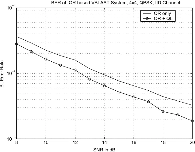
8 10 12 14 16 18 20 10−3

10−2 10−1

BER of QR based VBLAST System, 4x4, QPSK, IID Channel

SNR in dB

Bit Error Rate

QR only QR + QL

Figure 3.6: Bit error rate of QR based VBLAST system in IID random channel.

8 10 12 14 16 18 20

10−3 10−2 10−1

SNR in dB

Bit Error Rate

QR no ordering QR−Opt

(57)

8 10 12 14 16 18 20 10−3

10−2 10−1

SNR in dB

Bit Error Rate

QR+QL no ordering QR+QL−Opt

Figure 3.8: Effect of optimal ordering and backward/forward sweep on bit error rate.

8 10 12 14 16 18 20

1 2 3 4 5 6 7 8

SNR in dB

Throughput of QR−based VBLAST System, 4x4, QPSK, IID Channel

QR−no ordering QR−opt ordering QR+QL−no ordering QR+QL−opt ordering

(58)

symbols in the optimal order can also help improve the BERs as shown in Fig. 3.7. However, the combined gain as shown in Fig. 3.8 is not so impressive. Using only the forward sweep and optimal ordering can result in almost the same BER as using both sweeps and optimal ordering. Throughput results are shown in Fig. 3.9.

3.12.2 Execution Time

(59)

2 4 6 8 10 12 14 16 102

103 104 105 106

Complexity, VBLAST method vs QR method

MIMO System Size (axa)

Operations Count

VBLAST QR

Figure 3.10: Theoretical complexity of the VBLAST and QR methods.

2 4 6 8 10 12 14 16

102 103 104

Execution Time, VBLAST vs QR

Execution time in Sec

VBLAST QR

(60)

New Detection Method for VBLAST

Chapter Abstract

This chapter is one of the two major contributions of this thesis. The chapter introduces a new detection method for the VBLAST system based on a relatively less known matrix decomposition, the Polar Decomposition (PD). Section 4.1 introduces the PD, and sections 4.2 and 4.3 discuss the use of Cholesky and QR factorizations in addition to the PD for decoding VBLAST signals. The issue of optimal ordering is covered in section 4.4. Section 4.5 lists the properties of the PD, and section 4.6 shows how these properties are conducive to VBLAST detection. Two known algorithms for the PD are reviewed in section 4.7 with complexity analysis in section 4.8. The chapter ends with some simulation results and comments.

(61)

4.1 The Polar Decomposition

Every matrix H ∈ Cr×t

can be expressed as H = UP with U unitary and P positive semidefinite Hermitian. The matrixP is unique andU is also unique for a nonsingular

H [17]. This is known as the Polar Decomposition.

Using the Polar Decomposition, the MIMO transmission equation (3.2.1) can be written as

y=UPx+n. (4.1.1)

Premultiplying both sides by U′_{, one finds that}

U′y=Px+U′n (4.1.2)

which is equivalent to

˜

y=Px+ ˜n (4.1.3)

where we have y˜ = U′_y _and _n_˜ ₌_U′_n_{. Since,} _U _{is unitary,} _y_˜ _and _n_˜ _{have the same} distributions as y and n, respectively.

It is shown later that the equivalent system of (4.1.3) can be solved ( i.e, the transmitted vector xcan be estimated) with less computational cost if the properties of P are exploited.

4.2 Detection Using the Cholesky Factorization

The Cholesky factorization of a Hermitian positive definite matrix P is P =S′_S _with

(62)

triangular system

S−′y˜ =S−′{S′Sx+ ˜n}=Sx+ ˜n˜ (4.2.1)

where S−′

denotes the Hermitian of the inverse of S and n˜˜ = S−′

˜

n. Though this process would give the solution, it requires the matrix P to be nonsingular. The channel matrix H is often near-rank deficient, and so the Cholesky decomposition is likely to fail occasionally.

4.3 Detection Using the QR Factorization

Equation (4.1.3) can also be solved by computing a QR decomposition of the Hermitian matrix P =QR. With the channel matrix H decomposed in Polar form and then the matrix P in QR form, one writes (3.2.1) as

y=UQRx+n. (4.3.1)

Filtering the received vectory first throughU′ _{and then through}_Q′_{, one has an upper} triangular system

˜

y=Q′U′y=Rx+ ˜n. (4.3.2)

In explicit form, letting r=t=a

          ˜ y1 ˜ y2 ˜ y3 ... ˜ ya           =          

r11 r12 · · · r1a

0 r22 · · · r2a

0 0 · · · r3a

... ... ... ... 0 0 · · · raa

                    x1 x2 x3 ... xa           +           ˜ n1 ˜ n2 ˜ n3 ... ˜ na           . (4.3.3)

Then the a-th received symbol is

˜

(63)

Hence the a-th decision statistic da is

da=

1

raa

˜

ya =xa+

1

raa

˜

na. (4.3.5)

Once a decision (hard or soft) is made on da, it is assumed that the decision is

correct (i.e, the estimatexˆa is the same as xa) and its effect is subtracted from yet to

be detected symbols. The (a−1)-th decision statistic is then (assuming xˆa=xa)

da−1 =xa−1+

1

ra−1,a−1

˜

na−1. (4.3.6)

In general the i-th decision statistic is

di =

1

rii

˜

yi− a

X

j=i+1

rijxˆi

!

. (4.3.7)

4.4 Optimal Ordering

Following the same philosophy as VBLAST, the symbols can be detected in order of decreasing SNR. Because the last symbol is detected first in this method, one would like the last symbol to be the best one. This requires rearranging the columns of H

in increasing order of 2-norm (and also the rows of vector y) so that the last symbol corresponding to the last column gets detected first and so on. The optimal ordering can be determined just by comparing the diagonal elements ofP. Because, the largest diagonal entry of P corresponds to the strongest symbol.

4.5 Properties of the Polar Decomposition

(64)

• The Polar Decomposition can be computed from the Singular Value Decomposi-tion. Conversely, given the Polar Decomposition a spectral decomposition of P

will result in the Singular Value Decomposition.

• The unitary matrix U of the Polar Decomposition is the nearest unitary matrix to H where the distance is measured using the Frobenius norm.

• The Hermitian matrix P is the nearest Hermitian positive semidefinite matrix to

H where the distance is measured using 2-norm.

4.6 Behavior of Q and P Matrices

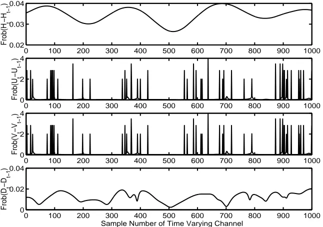
One nice feature of the Polar Decomposition is that the matrices Q and P do not change abruptly for a slowly varying channelH. This in contrast to a conventional QR decomposition. Fig. 4.1 shows the relative change in theQandP matrices for a slowly varying channel corresponding to FdT = 0.002, a typical indoor environment. This

nature of gradual change could enable tracking Q and P without requiring repetitive calculation. The possibility of tracking is a subject for further research and is not explored in this study.

4.7 Algorithms for the Polar Decomposition

(65)

0 100 200 300 400 500 600 700 800 900 1000 0.025 0.03 0.035 0.04 Frob(H t −H t−1 )

0 100 200 300 400 500 600 700 800 900 1000

0 0.05 0.1 Frob(U t −U t−1 )

0 100 200 300 400 500 600 700 800 900 1000

0.015 0.02 0.025 0.03 Frob(P t −P t−1 )

Sample Number of Time Varying Channel

Figure 4.1: Polar Decomposition behavior

UpPp is the Polar Decomposition, then Up and Pp can found by

Up =UsVs′

Pp =VsDsVs′

. (4.7.1)

4.7.1 Higham’s Algorithm for Polar Decomposition

In addition, there are algorithms that can compute the Polar Decomposition directly from a given matrix. One such algorithm is described by Higham [17] is as follows.

Here H is the given matrix. It is assumed H is square and nonsingular. For rectangular and singular matrices the algorithm can be modified. The parameter δ is the convergence tolerance.

• initialization

1. X0 =H

(66)

• iteration

1. k=k+ 1

2. γk= ||X− 1

k ||1||X− 1

k ||inf/(||Xk||1||Xk||inf)

1₄

3. Xk+1 = 1 2

γkXk+X−

′

k /γk

4. until ||XK+1−Xk||1 ≤δ||Xk+1||1

5. U =Xk+1

6. P = 1 2(U

∗_H₊_H∗_U₎

7. go to step 1

The algorithm is based on the classical Newton’s iteration to find the square root of a number. With the initialization X0 =H, the new Xk is computed as

Xk+1 =

1 2

γkXk+X−

′

k /γk

. (4.7.2)

Here γk is just an acceleration parameter. The convergence analysis of this algorithm

is given in [19].

(67)

4.8 Complexity Analysis

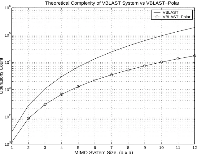
The main computational burden of the proposed method lies in the computation of the Polar Decomposition and the QR factorization. The Polar Decomposition can be found from the SVD of H with a cost of 22a3

operations assuming the SVD is computed using the Golub-Reinsch algorithm (R-SVD costs 26a3

). The direct iterative algorithm for Polar Decomposition due to Higham [18] converges in an average of 8 iterations spending 8a3

complex operations. This study uses the Higham method. On top of this, the QR factorization costs2a3

operations while the filtering byU′ _and _Q′ _{can be} done merely at a cost of 2a2

operations. The operations in the back substitutions in (4.4.2) are not counted because the VBLAST method has a similar computation which is ignored. So the total cost of this method is expected to be 10a3

+ 2a2

.

4.9 Simulation Results

4.9.1 BER, BLER and Throughput

The BER performance of the Polar Decomposition-based VBLAST is shown in Fig. 4.2. As seen, the optimal ordering, here also, produces slightly better BER. The Block Error Rate and Throughput are shown in Figs. 4.3 and 4.4 respectively. Further results are given in Chapter 6.

(68)

8 10 12 14 16 18 20 10−3

10−2 10−1

BER of Polar Decomposition−based VBLAST, 4x4, IID Channel

SNR in dB

Bit Error Rate

Polar+QR−no ordering Polar+QR−opt ordering

Figure 4.2: Bit error rate of Polar Decomposition-based VBLAST.

Polar Decomposition.