A multi block alternating direction method with parallel splitting for decentralized consensus optimization

R E S E A R C H

Open Access

A multi-block alternating direction method

with parallel splitting for decentralized

consensus optimization

Qing Ling

, Min Tao

, Wotao Yin

and Xiaoming Yuan

Abstract

Decentralized optimization has attracted much research interest for resource-limited networked multi-agent systems in recent years. Decentralizedconsensusoptimization, which is one of the decentralized optimization problems of great practical importance, minimizes an objective function that is the sum of the terms from individual agents over a set of variables on which all the agents should reach a consensus. This problem can be reformulated into an

equivalent model with two blocks of variables, which can then be solved by the alternating direction method (ADM) with only communications between neighbor nodes. Motivated by a recently emerged class of so-calledmulti-block ADMs, this article demonstrates that it is more natural to reformulate a decentralized consensus optimization problem to one with multiple blocks of variables and solve it by a multi-block ADM. In particular, we focus on the multi-block ADM with parallel splitting, which has easy decentralized implementation. Convergence rate is analyzed in the setting of average consensus, and the relation between two-block and multi-block ADMs are studied. Numerical experiments demonstrate the effectiveness of the multi-block ADM with parallel splitting in terms of speed and communication cost and show that it has better network scalability.

Introduction

In recent years, the communication, signal processing, control, and optimization communities have witnessed considerable research efforts on decentralized optimiza-tion for networked multi-agent systems [1-3]. A net-worked multi-agent system, such as a wireless sensor network (WSN) or a networked control system (NCS), is composed of multiple geographically distributed but interconnected agents which have sensing, computation, communication, and actuating abilities. This system gen-erally has limited resources for communication, since battery power is limited and recharging is difficult, while communication between two agents is energy-consuming. Furthermore, the communication link is often vulnera-ble and bandwidth-limited. In this situation, decentralized optimization emerges as an effective approach to improve network scalability. In decentralized optimization, data and computation are decentralized. Each agent exchanges

*Correspondence: [email protected]

1Department of Automation, University of Science and Technology of China, Hefei, Anhui, China

Full list of author information is available at the end of the article

information with its neighbors and accomplishes an oth-erwise centralized optimization task.

This article focuses on thedecentralized consensus opti-mization problem. We consider a network of L agents which cooperatively optimize a separable objective func-tion [3-8]:

min

L

i=1

fi(x), (1)

wherefi(x) : RN → Ris a convex function known to

agentionly. The goal is to minimize the objective subject to consensus onx.

Related study

The decentralized consensus optimization formulation (1) arises in many practical applications, such as averaging [9-11], estimation [12-17], learning [18-21], etc. The form offi(x) can be least squares [11-13],1-regularized least squares [14-17], or more general ones [18-21]. Note that this model can be extended to account for those with separable constraints, such as the network utility maxi-mization (NUM) problem [22-24].

Existing approaches to solving (1) include: i) belief prop-agation based on graphical models and Markovian ran-dom fields [18-20]; ii) incremental optimization which minimizes the overall objective function along a pre-defined path on the network [7,8]; iii) stochastic opti-mization with information exchange between neighboring agents [4-6]; and iv) optimization with explicit consen-sus constraints which can be handled with the alternating direction method (ADM) [3,12-17]. The ADM approach is fully decentralized, does not make any assumptions on network infrastructure such as free of loop or with a pre-defined path, and generally has satisfactory convergence performance. In this article, we mainly discuss the applica-tion of ADMs in the decentralized consensus optimizaapplica-tion problem.

Our research is along the line of information-driven signal processing and control of WSNs and NCSs [24-26]. Accompanied with the unprecedented data col-lection abilities offered by large-scale networked multi-agent systems, a new challenge also arises:how should we process such a large amount of data to make estimates and produce control strategies given limited network resources? Instead of processing the data in a fusion center, our solu-tion is letting each agent autonomously make decisions aided by limited communication with its neighbors. From this perspective, each individual objective function fi(x)

in (1) is constructed from the data collected by agent i, and x is the global information common to all agents (e.g., estimates or control strategies) obtained based on the data collected by the whole network. Though this framework can be generalized to various signal processing and control problems, this article focuses on those can be formulated as (1). For problems such as dynamic control and Kalman filtering of networked multi-agent systems, interested readers are referred to [1,2,27,28], respectively.

Our contribution

Motivated by a series of recent articles on multi-block ADMs and their convergence analysis [29-31], this article describes their applications to the decentralized consen-sus optimization problem. The multi-block ADM with parallel spliting is reviewed in Section 3. Unlike the clas-sical ADM (see textbooks [32,33]), this multi-block ADM splits the optimization variables intomultipleblocks and sequentially updates just one of them while fixing the others. The classical ADM, on the other hand, only has two blocks of variables. Hence in this article we refer to it by the two-block ADM. Our problem (1) does not naturally have two distinct blocks of variables, and to apply the two-block ADM one needs to introduce extra variables (see e.g., [15,16,32]). We review this in Section 2. On the other hand, it is simpler to apply the multi-block ADM to (1) and the resulting algorithm is readily decentralized.

In this article also analyzes the convergence rate of the multi-block ADM applied to the average consensus prob-lem, which is a special case of (1) wherefi(x)= ₂1x−bi2₂

for all i. In this setting, if the parameters of the multi-block ADM satisfy a certain formula, it is equivalent to the two-block ADM. Therefore, the two-block ADM can be considered as a special case of the multi-block ADM on average consensus problems. This relation also gives a guideline to select the parameters of the multi-block ADM so that it is not equivalent to and runs faster than the two-block ADM on all the tested decentralized con-sensus optimization problems, including the tested aver-age consensus problems. The simulation results demon-strate that the multi-block ADM accelerates convergence, reduces communication cost, and thus improves network scalability.

Paper organization

The rest of this article is organized as follows. Section 2 reviews a reformulation of the decentralized consensus optimization problem (1), to which the two-block ADM is applied. Section 3 reviews the multi-block ADM and applies a parallel-splitting version of it to (1). Section 4 elaborates on the convergence rate analysis on the average consensus problem, and shows that the two-block ADM is a special case of the multi-two-block ADM in this case. Section 5 presents numerical simulations of the two-block and multi-block ADMs. Finally, Section 6 concludes the article. Appendix 1 is placed in the last section.

Problem formulation and the two-block ADM In this section, we describe an equivalent formulation of the decentralized consensus optimization problem (1) and outline the algorithm design based on the two-block ADM.

Problem formulation

We consider a networked multi-agent system described by an undirected connected communication graphG = (L,E), whereLis the set ofLvertexes (distributed agents) and E is the set of edges (communication links). There exists an edge (i,j) ∈ E between agents i andj if they can directly communicate with each other. The two agents are also called one-hop neighbors, or simply neighbors. The set of one-hop neighbors of agentiis denoted byNi,

whose cardinality is denoted by|Ni|.

min

L i=1

fi(x(i)),

s.t. x(i)=x(j), ∀j∈Ni,∀i.

(2)

The two-block ADM

Let us consider the following convex program with sepa-rable equality constraints:

min g1(θ1)+g2(θ2), s.t. D1θ1+D2θ2=e.

(3)

Here fori = 1 and 2,gi : RN

i → R_{is convex,Di} ∈ RM×Ni_{, e} ∈ RM_{. The two-block ADM constructs the}

augmented Lagrangian function as:

La(θ1,θ2,λ)=g1(θ1)+g2(θ2)+λT(D1θ1+D2θ2−e)

+ c

2||D1θ1+D2θ2−e|| 2 2.

Hereλ∈RMis a Lagrange multiplier andcis a positive constant. At thetth iteration, the two-block ADM updates the optimization variablesθ1(t+1)andθ2(t+1)as:

θ1(t+1)=arg min

θ₁ La(θ1,θ2(t),λ(t)), θ2(t+1)=arg min

θ2

La(θ1(t+1),θ2,λ(t)),

and updates the Lagrange multiplierλ(t+1)as: λ(t+1)=λ(t)+c(D1θ1(t+1)+D2θ2(t+1)−e). The two-block ADM guarantees global convergence for any c > 0 [32]. More precisely, when eachgi is convex

fori= 1 and 2, the dual sequence{λ(t)}converges to an optimal dual solution of (5); if further the primal sequence

θ₁(t)T,θ₂(t)TT

is bounded, the sequence converges to an optimal primal solution of (5).

The two-block ADM for decentralized consensus optimization

The two-block ADM cannot be directly applied to prob-lem (2) because its constraints interconnect all the vari-ables pair by pair. There are no obvious two blocks. To overcome this, [32] describes a new block of auxiliary variables, and reformulates (2) as:

min

{x(i)_},{zij}

L

i=1 fi(x(i)),

s.t. x(i)=zij,x(j)=zij,∀j∈Ni,∀i.

(4)

Herezijis an auxiliary variable attached tox(i)andx(j).

Treating{x(i)} and{zij} as two blocks of variables, the

two-block ADM is applied to problem (4). This technique has been adopted in [15,16] to solve the decentralized con-sensus optimization problem with neighboring consen-sus constraints. After eliminating{zij}from the iterative

updates and further simplifications, the two-block ADM for (4) is given below as algorithm TB-ADM.

Initialization:Each agenti initializesx(i)₍₀₎₌₀

andαi(0)=0.

Step 1:At timet, each agenti updates its local copy

x(i)_as:x(i)_{(t+1)=arg min}

x(i) fi(x

(i)_)+αT

i (t)x(i)+

c

j∈Ni

||x(i)− 1₂x(i)(t)+x(j)(t) ||2₂, whereαiis the

Lagrange multiplier andc is a positive constant.

Step 2:At timet, each agenti updates its Lagrange

multiplierαias:

αi(t+1)=αi(t)+c|Ni|x(i)(t+1)−c j∈Ni

x(j)_(t+1).

Step 3:Repeat Step 1 and Step 2 until convergence.

TB-ADM is well suited for decentralized computation since the updates require only communication between agents i and j, who are one-hop neighbors. Detailed derivation of TB-ADM can be found in [15,16,32].

The multi-block ADM

The fact that many practical optimization problems nat-urally have multiple blocks of variables motivates the development of a class of multi-block ADMs, such as the one with parallel splitting [29], with prediction-correction [30], and with Gaussian back substitution [31]. Due to the nature of the decentralized consensus optimization prob-lem (2) and the need of parallelization, we choose the multi-block ADM with parallel splitting in [29].

The multi-block ADM with parallel splitting

Consider an equality constrained convex program which can be separated toLparts:

min

L i=1

gi(θi),

s.t. L

i=1

Diθi=e.

(5)

Here for alli,gi : RN

i → R_{is convex,Di} ∈ RM×Ni_, e ∈RM. At thetth iteration, the multi-block ADM with parallel splitting works as follows:

Step 1: Updating an auxiliary variable q:

q(t+1)=λ(t)+β

_L

i=1

Diθi(t)−e

,

Step 2: Updating optimization variables{θi}:

θ_i(t+1)=arg min θi

gi(θi)+q(t+1)TDiθi

+ μ

2||Diθi−Diθi(t)|| 2 2, ∀i,

whereμis a positive constant.

Step 3: Updating the Lagrange multiplierλ:

λ(t+1)=λ(t)+β

_L

i=1

Diθi(t+1)−e

.

The multi-block ADM guarantees global convergence if the two positive constantsβ andμare properly chosen. For the convergence proof and the settings ofβandμ, the interested reader is referred to [29].

The multi-block ADM for decentralized consensus optimization

Applying the multi-block ADM in (2) directly gets a decentralized algorithm, and does not need to introduce a new block of auxiliary variables and eliminate them, as we have done in the two-block ADM. We provide the algorithm to solve (2) based on the multi-block ADM with parallel splitting, denoted as MB-ADM. Detailed derivation of MB-ADM is given in Appendix 1.

Initialization:Each agenti initializesqi(0)=0,

x(i)(0)=0, andλ_i(0)=0.

Step 1:At timet, each agenti updates its auxiliary

variableqias:

qi(t+1)=λi(t)+β|Ni|x(i)(t)−β j∈Ni

x(j)(t), where

βis a positive constant.

Step 2:At timet, each agenti updates its local copy

x(i)as:x(i)(t+1)=arg min

x(i) fi(x

(i)_)+2qT

i (t+1)x(i)+

μ|Ni|||x(i)−x(i)(t)||2₂, whereμis a positive constant.

Step 3:At timet, each agenti updates its Lagrange

multiplierλias:

λi(t+1)=λi(t)+β|Ni|x(i)(t+1)−β j∈Ni

x(j)_(t+1).

Step 4:Repeat Step 1 to Step 3 until convergence.

In each iteration, to update qi(t+1) and λi(t), agent ineedsx(j)_{(t)with the size ofN ×1 from all neighbors} j ∈ Ni; to optimizex(i)(t+1), agenti only needs local

information qi(t+1) andx(i)(t). In all, each agent only

needs to broadcast anN×1 vector of its local copy (i.e., x(i)(t)) to its neighbors per iteration. MB-ADM and TB-ADM have the same per-iteration communication cost. At thetth iteration, agentineeds to updatex(i)(t),qi(t),

andλi(t)in its memory for MB-ADM. Hence the memory

requirement is slightly higher than that of TB-ADM, for which onlyx(i)(t)andαi(t)need to be updated.

Convergence rate analysis

Convergence rate is an significant issue for decentralized algorithms, since it directly influences the overall com-munication cost. With respect to general separable con-vex programs, [29,34] proves the sublinear convergence rates of ∼ 1_t for the multi-block and two-block ADMs, respectively. However, when they are applied to the aver-age consensus problems, much faster convergence can be observed. For this reason, we improve the convergence rate in this section.

The average consensus problem gives rise to problem (2) withfi(x(i))= 1₂||x(i)−bi||22,∀i[9-11]; namely, agents aims at averaging their original measurements{bi}via one-hop

communication. Without loss of generality, we assume thatx(i)andbiare both scalars since their dimensions have

no effect on the convergence rate.

Convergence rate of MB-ADM

In analyzing the convergence rate of MB-ADM for the average consensus problem, we first rewrite MB-ADM as a state transition equation form and then use the spectral analysis tools to provide a bound of convergence rate. Our train of thought is similar to that in [35] for the two-block ADM.

According to the derivation in Appendix 1, we can rewrite MB-ADM in a state transition equation form. Let us define a state vectorsM(t+1)=[x(1)(t+1),. . .,x(L)(t+

1),x(1)(t),. . .,x(L)(t)]T and the corresponding state tran-sition equation of MB-ADM is:

sM(t+1)=MsM(t). (6)

Here the state transition matrixMis defined as:

M =

M M

IL×L 0L×L

with _M being an L × L matrix whose (i,i)th entry is 1−4β₁₊|N₂i|+_μ|N4μ_i||Ni| and (i,j)th entry is ₁₊₂4_μβ_|Ni| if i and j are neighbors, and T being an L × L matrix

whose (i,i)th entry is 2β|₁N₊i|−_2μ2_|Nμ|_i|Ni| and (i,j)th entry is −₁₊₂2_μβ_|Ni| if i and j are neighbors. We can see that summation of each row of M is 1. The initial

state is sM(1) =[₁₊₂bμ1|N1|,. . .,

bL

1+2μ|NL|, 0,. . ., 0] when

each agent i initializes qi(0) = 0, x(i)(0) = 0, and

λ_i(0)=0.

Proposition 1.(convergence and convergence rate of

MB-ADM on average consensus) The state transition

Property 1.The matrixMhas an eigenvalueρM1=1 with multiplicity 1, and its corresponding left and right eigenvectors are:

respectively. Note thatlM1andrM1are chosen subject to lM1rM1=1.

Further, denoting thatκMis the size of the largest Jordan

block ofM, the convergence rate is: ||sM(t+1)−sM(∞)||2∼t(κM−1)ρMt .

Proof of Property 1 is given in Appendix 1. Property 2 comes from the classical convergence rate analysis of state transition equations. IfρM1 = 1 andρM < 1, then

there exists a unique sM(∞) and the convergence rate

is||sM(t+ 1) −sM(∞)||2 ∼ t(κM−1)ρtM (see [36], Fact

3). Next we try to find one possible (and hence unique) sM(∞). By definition,MrM1 = ρM1rM1 = rM1. Hence limt→∞tMrM1 =rM1. Similarly, limt→∞lM1M =lM1. These two facts mean thatrM1lM1is a possible limit point of limt→∞tM. Therefore,rM1lM1sM(1)is a possible (and

hence unique) limit point ofsM(∞).

Remark 1.Note that the∼t(κM−1)ρt_Mrate, though still

loose, is tighter than the∼ 1_t rate of the multi-block ADM for general separable convex programs [29]. Indeed, from numerical experiments, we find thatκM, the size of the

largest Jordan block ofM, is often equal to 1 (it means

thatM is diagonalizable). In this case, the convergence

rate can be as fast as∼ρ_Mt .

In Property 2, there is a condition thatρM<1. It is not

necessarily for true any choices ofμandβ. Next we show two nontrivial special cases where the condition in Prop-erty 2 satisfy. The first special case connects MB-ADM with TB-ADM. Analysis of these two special cases as well as numerical simulations provide guidelines for parameter selection in MB-ADM.

Proposition 2.(two nontrivial special cases) We have

ρm<1 in either one of the following two cases:

Case 1: The parameters μand β are chosen such that μ= 2β > 0; further, ₁₊2β₂|_μN_|Nj|

Case 2: The parameters μand β are chosen such that μ=β >0; further, ₁₊2β_2μ|N_|Nj|_j| < 1₂and₁₊2μ₂|_μN_|Nj|

j| < 1 2for all j=1, 2,. . .,L.

Remark 2.The proof of Proposition 2 is given in

Appendix 1. In case 1, we set μ = 2β > 0, which indeed leads to the equivalence between MB-ADM and TB-ADM, as we will show in the next subsection. In case 2, we setμ = β > 0, which brings faster convergence for the average consensus problem according to numer-ical simulations (see Section 5.2). Hence we recommend to set β = τ μ with a fixed ratio 1₂ ≤ τ ≤ 1, and just tune the value ofμ. This setting also works well for the general decentralized consensus optimization prob-lem (1). Tuningμfor MB-ADM is similar to tuningcfor TB-ADM; both algorithms have 1 parameter subject to the user choice. Note that the conditions in Proposition 2 are merely sufficient; ₁₊2β₂|_μN_|Nj|_j| and ₁₊2μ_2μ|N_|Nj|_j| can be larger than their upper bounds given above.

Connection between MB-ADM and TB-ADM

To show the connection between MB-ADM and TB-ADM, we also write TB-ADM as a state transition equation form. Note that [35] considers another kind of two-block ADM for the average consensus problem, where consensus constraints are quadratically penalized by different weights in the augmented Lagrangian func-tion. In TB-ADM, the consensus constraints are quadrat-ically penalized by the same weightc.

We define a state vector sT(t + 1) =[x(1)(t +

1),. . .,x(L)_{(t + 1),x}(1)_{(t),. . .,x}(L)_(t)]T _{and the}

corre-sponding state transition equation, according to the derivation in Appendix 1:

sT(t+1)=TsT(t). (7)

Here the state transition matrix_Tis defined as:

T = j are neighbors, and T being an L× L matrix whose

Comparing the state transition equations of MB-ADM and TB-ADM, we can find that TB-ADM is indeed a spe-cial case of MB-ADM whenc=μ=2β >0. In this sense, MB-ADM provides more flexibility in parameter selection than TB-ADM. According to our simulations in Section 5.2, settingβ = τ μwith 1₂ ≤ τ ≤ 1 makes MB-ADM faster than TB-ADM.

LetρTibe theith eigenvalue ofT. ApparentlyρT1=1. Defining:

ρ_T =max

i=1 |ρTi|,

and denotingκT as the size of the largest Jordan block of

T, we can prove that TB-ADM has a similar∼t(κT−1)ρ_Tt

convergence rate to the optimal solution given the condi-tions in Case 1 of Proposition 2. Interestingly, the upper bounds of₁₊2c₂|_cN_|Nj|_j| < 1₂for allj=1, 2,. . .,Lare no longer needed since TB-ADM guarantees global convergence for anyc>0.

Numerical Experiments

In this section, we present numerical simulations and demonstrate the performance of MB-ADM on the decen-tralized consensus optimization problems. Particularly, we are interested in how the communication cost scales to the network size.

Simulation Settings

In the numerical experiments, we consider the case that the agents cooperatively solve a least-squares problem. Each agentihas a measurement matrixAi ∈RM×N and

a measurement vectorbi ∈ RM. The objective function

in (1) is thus f(x) = _iL₌₁fi(x) = 1₂Li=1||Aix−bi||22. The elements of the true signal vectorx0and the entries of the measurement matrices{Ai}follow the normal

distri-butionN(0, 1). The measurement vectorbi = Aix0+ηi;

the elements of the noise vector η_i follow the normal distribution N(0, 0.1). In the tests of average consen-sus, {Ai} reduce to identity matrices and are no longer

random.

In the simulation, we assume that L agents are uni-formly randomly deployed in a 100×100 area. All agents have a common communication rangerC, which is chosen

such that the networked multi-agent system is connected. GivenrC, the average node degreedcan be calculated. We

consider the following three scenarios: #1)L=50,M=1, N =1,{Ai =1},rC = 30,d 12; #2)L= 50,M= 10, N = 5,rC = 30,d 12; #3)L = 200,M= 10,N = 5, rC =15,d12. Scenario #1 is the average consensus test.

Throughout the simulations, we setβ =τ μin MB-ADM withτ =0.9.

Convergence rate for average consensus

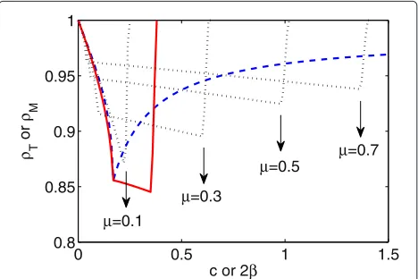
Under different choices ofc,μ, andβ, the values ofρTfor

TB-ADM and the values ofρMfor MB-ADM with respect

to scenario #1 are shown in Figure 1. For TB-ADM,ρT

sharply reduces whencincreases from 0; after a certain turning point (at c∗ 0.17) which corresponds to the fastest convergence rate,ρT steadily increases. The curve

ofρM for MB-ADM shows to be more complicated due

to the existence of two parameters,μandβ. For eachμ, ρ_Msteadily reduces whenβincreases from 0, then sharply goes to be larger than 1 which corresponds to divergence. The largerμ, the wider convergence range forβ; but the side-effect is the relatively slower convergence rate. The curve of particular interest to us isμ=c∗0.17. In this curve, 2β = c∗ 0.17 corresponds to Case 1 in Propo-sition 2; namely, when MB-ADM reduces to TB-ADM. Increasing β from c∗, ρM still decreases until reaching

a turning point 2β = 2c∗ 0.34, which corresponds to Case 2 in Proposition 2. This simulation validates our analysis in Section 5.2, as well as the proposed parameter selection rule (namely, setting a ratioτ, 1₂ ≤τ ≤1, such thatβ=τ μ).

Simulation results about the actual convergence prop-erties are shown in Figure 2. By absolute error we denote the₂-norm of the distance between the current solution and the centralized optimal solution. Though the conver-gence rates of MB-ADM and TB-ADM are at the same magnitude, MB-ADM shows to be slightly superior to TB-ADM.

According to the theoretical analysis in Sections 4.1 and 4.2, the estimated convergence rates of MB-ADM and TB-ADM are ∼ t(κM−1)_ρt

M and ∼ t(κT−1)ρTt, respectively.

However, numerical simulations show that they are loose bounds; the actual convergence rate, as we can observe from Figure 2, are linear.

0 0.5 1 1.5

0.8 0.85 0.9 0.95 1

c or 2β ρ T

or

ρ M

μ=0.1

μ=0.3

μ=0.5 μ =0.7

Figure 1Curves ofρTandρMfor TB-ADM MB-ADM in scenario

#1.The dash line is for TB-ADM and its turning point corresponds to

0 100 200 300 400 500 10−20

10−15 10−10 10−5 100

Iteration

Absolute Error

MB−ADM, μ=0.1 MB−ADM, μ=0.2 TB−ADM, c=0.1 TB−ADM, c=0.2

Figure 2Convergence of the decentralized consensus optimization algorithms for scenario#1.Hereβ=τ μwith

τ=0.9.

Performance Comparison

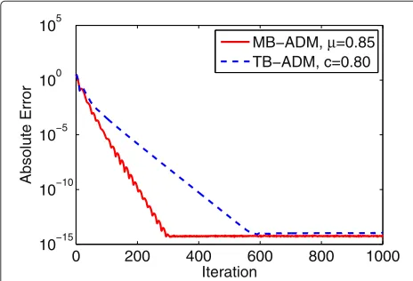
Figures 3 and 4 depict the convergence properties of the two decentralized consensus optimization algorithms for scenarios #2 and #3, respectively. The parametersμand c are tune to be near the best ones with. Here we still haveβ = τ μwithτ = 0.9. For either the medium net-work in scenario #2 or the large netnet-work in scenario #3, both algorithms linearly converge to the optimal solution. Comparing the two decentralized algorithms, MB-ADM outperforms TB-ADM in each scenario regarding conver-gence rate.

What of particular interest to us is whether the decen-tralized algorithms are scalable to network size. Observing Figure 3 withL=50 agents andd12, and Figure 4 with L= 200 agents andd 12, we can find that the conver-gence rates of the two algorithm are more dependent on the average node degree other than on the network size.

0 200 400 600 800 1000

10−15 10−10 10−5 100 105

Iteration

Absolute Error

MB−ADM, μ=0.85 TB−ADM, c=0.80

Figure 3Convergence of the decentralized consensus optimization algorithms for scenario#2.The parameterscandμ

are tuned to near the best, andβ=τ μwithτ=0.9.

0 200 400 600 800 1000

10−15 10−10 10−5 100 105

Iteration

Absolute Error

MB−ADM, μ=0.95 TB−ADM, c=0.90

Figure 4Convergence of the decentralized consensus optimization algorithms for scenario#3.The parameterscandμ

are tuned to near the best, andβ=τ μwithτ=0.9.

These numerical experiments verify the well-recognized claim that decentralized optimization may improve the performance of a networked multi-agent system with respect to network scalability.

Communication cost

Communication cost, in terms of energy consumption and bandwidth, is the major design consideration of a resource-limited networked multi-agent system, and can be approximately evaluated by the volume of information exchange during the decentralized consensus optimiza-tion process. Ignoring the extra burden of coordinating the network, for each agent, the communication cost is proportional to the number of iterations multiplied by the volume of information exchange per iteration. Therefore, reducing the information exchange per iteration is of crit-ical importance to the design of lightweight algorithms.

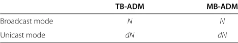
Comparing the two decentralized consensus optimiza-tion algorithms, the informaoptimiza-tion exchange per iteraoptimiza-tion is decided by the communication mode of agents, namely, broadcast or unicast. In the broadcast mode, one agent can send one piece of information to all of its neighbors with one transmission; contrarily, in the unicast mode, the agent needs multiple transmissions to do so. The two modes both have their pros and cons. The broadcast mode utilizes the characteristic of wireless communication, but may brings difficulties in coordinating the network, such as avoiding collisions. Though the unicast mode con-sumes much more transmissions, the randomized-gossip-like scheme is very useful in communication for the sake of robustness [37]. The average volume of information exchange per iteration of the four decentralized consensus optimization algorithms are outlined in Table 1, for both the broadcast and unicast modes.

Table 1 Average volume of information exchange per iteration

TB-ADM MB-ADM

Broadcast mode N N

Unicast mode dN dN

are scalable to the network size. Since the number of iterations is proportional to the average node degreed, the overall average volume of information exchange is

∼ Ndfor the broadcast mode and∼ Nd2for the unicast mode. As a comparison, consider a centralized networked multi-agent system uniformly randomly deployed in a two-dimensional area with a fusion center which collects measurement vectors from all agents. The average volume of information exchange is∼M√Lwhile the worst one is

∼MLfor agents near the fusion center. When the network size Lincreases, the communication cost caused by the centralized network infrastructure is unaffordable and the decentralized network infrastructure is hence superior.

Conclusion

This article considers solving the decentralized consensus optimization problem with the parallel version multi-block ADM in a networked multi-agent system. The tradi-tional ADM can be used but it requires the introduction of a second block of auxiliary variables whereas our method takes advantages of the problem’s nature of having multi-ple blocks of variables. We analyze the rate of convergence of our method applied to the average consensus prob-lem. Analysis results that the two-block ADM is a spe-cial case of the multi-block ADM on average consensus. With extensive numerical experiments, we demonstrate the effectiveness of the proposed algorithm.

In the implementation of a networked multi-agent sys-tem, practical issues such as packet loss, asynchronization, and quantization are inevitable. This article assumes that the communication links are reliable, the network time is slotted and well synchronized, and the exchanged infor-mation is not quantized. We would like to address these issues in future research.

Appendix 1

This section provides some theoretical results in the article.

Development of MB-ADM

The decentralized consensus optimization problem (2) with neighboring consensus constraints can be rewritten as the form of (5). Apparently,gi=fi,θi=x(i), andeis an L2_{N×1 zero vector. EachD}

iis anL2N×Nmatrix withL2

blocks ofN×Nmatrices. Each block ofDican be defined

as follows. Consider anL×LmatrixU(i)_{, whose(i,j)th} entryU_i(i_j) =1 ifj=iandi∈Ni,U_i(i_j) = −1 ifi=iand

j∈Ni, andU_i(i_j) =0 otherwise. The(i+Lj−L)th block ofDiisU_i(i_j)IN, whereINis anN×Nidentity matrix.

Sub-stituting them to the multi-block ADM, we can find that in optimizingx(i), agentionly needs its local information as well as part ofq; on the other hand, to update its corre-sponding part ofqandλ, each agent only needs based on the information from itself and its neighbors. The result-ing algorithm is hence fully decentralized due to the nice structure of{Di}.

At timet, the multi-block ADM works as follows:

Step 1: Updating the auxiliary variables{qij}:

qij(t+1)=λij(t)+β

x(i)(t)−x(j)(t)

, ∀i,∀j∈Ni.

(8) Step 2: Optimizing the local copies{x(i)}:

x(i)(t+1)=arg min

x(i) fi(x

(i)₎₊

j∈Ni

(qij(t+1)

−qji(t+1))Tx(i)+μ|Ni|||x(i)

−x(i)(t)||2₂, ∀i.

(9)

Step 3: Updating the Lagrange multipliers{λij}:

λij(t+1)=λij(t)+β

x(i)(t+1)−x(j)(t+1)

, ∀i,

∀j∈Ni.

(10) Note thatβandμare positive constant parameters used by the multi-block ADM.

The updating rules (8), (9), and (10) can also be fur-ther simplified. Since we often set {λij(0)} as 0, (8) and

(10) imply thatqij(t+1) = −qji(t+1)andλij(t+1) = −λji(t+1). Summing up the two sides of (8) and (10) and

defining a new auxiliary variableqi=j∈Niqijas well as

a new Lagrange multiplierλ_i = _j∈N

iλij, their updating

rules are:

qi(t+1)=λi(t)+β|Ni|x(i)(t)−β

j∈Ni x(j)(t),

(11)

λi(t+1)=λi(t)+β|Ni|x(i)(t+1)−β

j∈Ni

x(j)(t+1).

(12) Hence (9) simplifies to:

x(i)(t+1)=arg min

x(i) fi(x

(i)_)+2qT

i (t+1)x(i)+μ|Ni|||x(i) −x(i)(t)||2₂.

State transition equation of MB-ADM

Proof of Property 1 in Proposition 1

It is straightforward to show that ρM1 = 1 is an eigenvalue of _M, as well as lM1 and rM1 are its cor-responding left and right eigenvectors. Next we prove that ρ_M1 = 1 is with multiplicity 1 by contradiction. If ρ_M1 = 1 belongs to a larger Jordan block, there exists a vector [wT,w¯T]T, such that _M[wT,w¯T]T= [wT,w¯T]T+[ 1,. . ., 1, 1,. . ., 1]T. Herewandw¯ are both L × 1 vectors (see [36], Fact 2). Observing the lower half of M, apparently w¯ = w−[ 1,. . ., 1]T.

Sup-pose that wk has the largest real part among all

ele-ments ofw. Picking up thekth row ofM[wT,w¯T]T =

respectively. Recalling that Re(wk) ≥ Re(wj)and picking

up the real part of (18), we have: This leads to contradiction. Hence ρM1 = 1 is an eigenvalue ofMwith multiplicity 1.

Proof of Proposition 2

Denote the ith eigenvalue of i asρMi. Apparently, its

eigenvectors should have the form of [ρMivT,vT]Twhere vT=[v1,. . .,vL]Tis a nonzero vector, since the lower half

ofMis [IL×L, 0L×L]. Suppose thatvkhas the largest norm

or equivalently:

Sincevk has the largest norm among all elements ofv,

taking norms for the both sides of (21) leads to:

Notice that the inequalities turn to equalities when and only whenvj = vk,∀j ∈ Nk. Asvk has the largest norm

among all elements of v, any vj with j ∈ Nk also has

such inequalities, and the inequalities turn to equalities when and only whenvj = vj,∀j ∈ Nj. Because the

net-work is connected, we can deduce that these inequalities turn to equalities when and only when{vi}are all equal.

This corresponds to the eigenvalueρM1 = 1. Canceling |vk|from the both sides and definingd1 = ₁₊2β₂μ|N|Nk|k| and d2= ₁₊2μ₂|μN|Nk|k|, (22) is equivalent to:

|ρ_Mi2 −ρMi+2d1ρMi−d2ρMi−d1+d2| ≤ |2d1ρMi−d1|. (23)

Let us consider the two nontrivial special cases.

Case 1.The parametersμandβ are chosen such that

μ =2β >0; further, ₁₊2β₂|_μN_|Nj|_j| < ₄1and ₁₊2μ_2μ|N_|Nj|_j| < 1₂for

Case 2.The parametersμandβ are chosen such that

μ=β >0; further,₁₊2β₂|_μN_|Nj|_j| < ₂1and₁₊2μ_2μ|N_|Nj|_j| < 1₂for all

Let us prove the conclusion by contradiction. Suppose that there exists aρMiwith|ρMi| ≥1 satisfies (26), then:

Again, the inequalities turns to equalities only for ρM1=1. For any other eigenvalueρMi, we have|ρMi|<1

which contradicts with|ρ_Mi| ≥1. Therefore,|ρ_Mi|<1 for i=1.

the optimality condition forx(i)(t+1)is:

Considering x(i)(t), the optimality condition is corre-spondingly: Combining (28) and (29) with:

α_i(t+1)=α_i(t)+c|Ni|x(i)(t+1)−c

j∈Ni

x(j)(t+1),

the state transition equation for agentiis:

x(i)(t+1)=x(i)(t)+ 2c

The authors declare that they have no competing interests.

Acknowledgements

The work of Qing Ling is supported in part by NSFC grant 61004137 and Fundamental Research Funds for the Central Universities. The work of Wotao Yin is supported in part by ARL and ARO grant W911NF-09-1-0383 and NSF grants DMS-0748839 and ECCS-1028790. The work of Xiaoming Yuan is supported in part by the General Research Fund No. 203311 from Hong Kong Research Grants Council.

Author details

1_{Department of Automation, University of Science and Technology of China,}

Hefei, Anhui, China.2_{School of Science, Nanjing University of Posts and}

Telecommunications, Nanjing, Jiangsu, China.3_{Department of Computational}

and Applied Mathematics, Rice University, Houston, Texas, USA.4_Department

of Mathematics, HongKong Baptist University, Kowloon Tong, Hong Kong.

Received: 15 February 2012 Accepted: 5 October 2012 Published: 12 November 2012

References

1. W Ren, R Beard, E Atkins, Information consensus in multivehicle cooperative control: collective group behavier through local interaction. IEEE Control Systs. Mag.27, 71–82 (2007)

2. R Olfati-Saber, inProceedings of CDC. Kalman-consensus filter: optimality, stability, and performance, Shanghai, China, 2009), pp. 7036–7042 3. S Boyd, N Parikh, E Chu, B Peleato, J Eckstein, Distributed optimization and

statistical learning via the alternating direction method of multipliers. Foundation Trends Mach. Learn.3, 1–122 (2010)

4. J Tsitsiklis,Problems in decentralized decision making and computation. (MIT, Ph.D Thesis, 1984)

5. A Nedic, A Ozdaglar, Distributed subgradient methods for multi-agent optimization. IEEE Trans. Autom. Control.54, 48–61 (2009)

6. K Srivastava, A Nedic, Distrbited asynchronous constrained stochastic optimization. IEEE J. Sel. Topics Signal Process.5, 772–790 (2011) 7. M Rabbat, R Nowak, inProceedings of IPSN. Distributed optimization in

sensor networks, Berkeley, USA, 2004), pp. 20–27

8. M Rabbat, R Nowak, Quantized incremental algorithms for distributed optimization. IEEE J. Sel. Areas Commun.23, 798–808 (2006) 9. L Xiao, S Boyd, S Kim, Distributed average consensus with

least-mean-square deviation. J. Parallel Distrib. Comput.67, 33–46 (2007) 10. S Kar, J Moura, Distributed consensus algorithms in sensor networks:

quantized data and random link failures. IEEE Trans. Signal Process.58, 1383–1400 (2010)

11. A Olshevsky,Efficient Information Aggregation Strategies for Distributed

Control and Signal Processing. (Ph.D Thesis, MIT, 2010)

12. I Schizas, A Ribeiro, G Giannakis, Consensus in ad hoc WSNs with noisy links - Part I: distributed estimation of deterministic signals. IEEE Trans. Signal Process.56, 350–364 (2008)

13. G Mateos, I Schizas, G Giannakis, Distributed recursive least-squares for consensus-based in-network adaptive estimation. IEEE Trans. Signal Process.57, 4583–4588 (2009)

14. Q Ling, Z Tian, Decentralized sparse signal recovery for compressive sleeping wireless sensor networks. IEEE Trans. Signal Process.58, 3816–3827 (2010)

15. J Bazerque, G Giannakis, Distributed spectrum sensing for cognitive radio networks by exploiting sparsity. IEEE Trans. Signal Process.58, 1847–1862 (2010)

16. G Mateos, J Bazerque, G Giannakis, Distributed sparse linear regression. IEEE Trans. Signal Process.58, 5262–5276 (2010)

17. D Jakovetic, J Xavier, J Moura, Cooperative convex optimization in networked systems: augmented Lagrangian algorithms with direct gossip communication. IEEE Trans. Signal Process.59, 3889–3902 (2011) 18. M Cetin, L Chen, J Fisher I I I, A Ihler, R Moss, M Wainwright, A Willsky,

Distributed fusion in sensor networks. IEEE Signal Process. Mag.23, 42–55 (2006)

19. J Predd, S Kulkarni, V Poor, Distributed learning in wireless sensor networks. IEEE Signal Process. Mag.24, 56–69 (2007)

20. J Predd, S Kulkarni, H Poor, A collaborative training algorithm for distributed learning. IEEE Trans. Inf. Theory.55, 1856–1871 (2009) 21. U Khan, S Kar, J Moura, Higher dimensional consensus: learning in

large-scale networks. IEEE Trans. Signal Process.58, 2836–2849 (2010) 22. A Jadbabaie, A Ozdaglar, M Zargham, inProceedings of CDC. A distributed

Newton method for network optimization, Shanghai, China, 2009), pp. 2736–2741

23. J Koshal, A Nedic, U Shanbhag, Multiuser optimization: distributed algorithms and error analysis. SIAM J. Optimiz.21, 1046–1081 (2011) 24. P Wan, M Lemmon, inProceedings of ACC. Distributed network utility

maximization using event-triggered augmented Lagrangian methods, St. Louis, USA, 2009), pp. 3298–3303

25. F Zhao, J Shin, J Reich, Information-driven dynamic sensor collaboration. IEEE Signal Process. Mag.19, 61–72 (2002)

26. F Zhao, L Guibas,Wireless Sensor Networks: an Information Processing

Approach. (Morgan Kaufmann, Burlington, USA, 2004)

27. I Schizas, G Giannakis, S Roumeliotis, A Ribeiro, Consensus in ad hoc WSNs with noisy links – part II: distributed estimation and smoothing of random signals. IEEE Trans. Signal Process.56(4), 1650–1666 (2008)

28. A Ribeiro, I Schizas, S Roumeliotis, G Giannakis, Kalman filtering in wireless sensor networks: reducing communication cost in state estimation problems. IEEE Control Systs. Mag.30, 66–86 (2010)

29. M Tao, Some parallel splitting methods for separable convex programming withO(1/t)convergence rate. in press

30. B He, M Tao, M Xu, X Yuan, Alternating directions based contraction method for generally separable linearly constrained convex programming problems. in press

31. B He, M Tao, X Yuan, Alternating direction method with Gaussian back substitution for separable convex programming. SIAM J. Optim.22, 313–340 (2012)

32. D Bertsekas, J Tsitsiklis,Parallel and Distributed Computation: Numerical

Methods, 2nd edn. (Athena Scientific, Nashua, USA, 1997)

34. B He, X Yuan, On theO(1/n)convergence rate of Douglas-Rachford alternating direction method. SIAM J. Num. Anal.50, 700–709 (2012) 35. T Erseghe, D Zennaro, E Dall’Anese, L Vangelista, Fast consensus by the

alternating direction multipliers method. IEEE Trans. Signal Process.59, 5523–5537 (2011)

36. J Rosenthal, Convergence rates for Markov chains. SIAM Rev.37, 387–405 (1995)

37. S Boyd, A Ghosh, B Prabhakar, D Shah, Randomized gossip algorithms. IEEE Trans. Inf. Theory.52, 2508–2530 (2006)

doi:10.1186/1687-1499-2012-338

Cite this article as:Linget al.:A multi-block alternating direction method

with parallel splitting for decentralized consensus optimization.EURASIP Journal on Wireless Communications and Networking20122012:338.

Submit your manuscript to a

journal and benefi t from:

7Convenient online submission 7Rigorous peer review

7Immediate publication on acceptance 7Open access: articles freely available online 7High visibility within the fi eld

7Retaining the copyright to your article