R E S E A R C H
Open Access
Robust SINR-constrained MISO downlink
beamforming: when is semidefinite
programming relaxation tight?
Enbin Song
1*, Qingjiang Shi
2, Maziar Sanjabi
3, Ruo-Yu Sun
3and Zhi-Quan Luo
3Abstract
We consider the multiuser beamforming problem for a multi-input single-output downlink channel that takes into account the errors in the channel state information at the transmitter side (CSIT). By modeling the CSIT errors as elliptically bounded uncertainty regions, this problem can be formulated as minimizing the transmission power subject to the worst-case signal-to-interference-plus-noise ratio constraints. Several methods have been proposed to solve this nonconvex optimization problem, but none can guarantee a global optimal solution. In this article, we consider a semidefinite relaxation (SDR) for this multiuser beamforming problem, and prove that the SDR method actually solves the robust beamforming problem to global optimality as long as the channel uncertainty bound is sufficiently small or when the transmitter is equipped with at most two antennas. Numerical examples show that the proposed SDR approach significantly outperforms the existing methods in terms of the average required power consumption at the transmitter.
Introduction
Consider the transmit beamforming problem in a multi-user multi-input single-output (MISO) downlink channel where the transmitter equipped with multiple-antennas sends independent data steams to a number of receivers, each having a single receive antenna. For such a system, a popular measure of quality of service (QoS) is the signal-to-interference-plus-noise ratio (SINR) [1] and optimal downlink transmit beamforming can be formulated as minimizing the transmission power subject to the SINR constraints.
It is well known that if the perfect channel state infor-mation is available at the transmitter (CSIT), the optimal transmit beamforming problem can be solved efficiently via convex optimization [1-4]. However, perfect CSIT is impossible to obtain in practice due to the finite length of training signal and/or limited feedback band-width [5,6]. This is unfortunate, because we cannot simply ignore the CSIT imperfection in the design of downlink
*Correspondence: [email protected]
1Department of Mathematics, Sichuan University, Chengdu, Sichuan 610064, China
Full list of author information is available at the end of the article
beamformers, for otherwise the resulting solution might violate the SINR constraints for some users.
As a remedy, various researchers have proposed robust beamforming formulations by taking the CSIT imper-fection into consideration. There are two major types of robust downlinks beamforming design: the stochastic robust design and the worst-case robust design. For the stochastic robust beamforming design (see [7-13]), the CSIT errors are modeled as random variables with known statistical properties. In this case, the design goal of transmit beamforming is to minimize transmission power while ensuring that all the receive SINR requirements are satisfied with high probability. In contrast, the worst-case robust beamforming design (see [14-20]) assumes that the CSIT errors belong to some known bounded uncer-tainty sets. The robust beamforming vectors are designed to satisfy the SINR requirements for all possible chan-nel realizations in the uncertainty regions. For instance in [18,19], the authors formulated the robust beamform-ing problem as minimizbeamform-ing the transmission power sub-ject to the worst-case SINR constraints, while assuming the CSIT errors lie in some elliptically bounded regions.
Unfortunately the resulting robust downlink beamform-ing problem is nonconvex and has infinitely many con-straints. It is difficult to solve in practice.
To overcome the computational difficulties associated with the robust downlink beamforming, researchers have proposed various optimization methods to approximate the problem by restricting the non-convex feasible region to a smaller but convex set [18,19]. Due to convex restric-tion, these methods typically can not find the globally minimum transmission power although they do guarantee the satisfaction of the QoS constraints. In fact, the com-puted beamforming solutions can be highly suboptimal.
In this article, we consider a semidefinite programming relaxation (SDR) method to solve the worst-case robust downlink beamforming problem for the MISO channel system. The SDR method has been extensively used in addressing the robust beamforming problem [21,22]. A critical issue of SDR is whether it can exactly solve the original problem, which is equivalent to whether the method can produce a rank-one solution. The key result of this article is that the robust beamforming problem can be globally solved by SDR method (i.e., SDR is tight) under elliptically bounded CSI errors, provided that the size of channel errors is sufficiently small or if the trans-mitter is equipped with no more than two antennas. We give a computable bound which ensures the tightness of the SDR if the radius of the error region is less than this bound. In the simulations, this computable bound is always reasonably large, which makes the tightness result valuable. Moreover, the SDR method significantly outper-forms the existing robust beamforming methods based on the worse-case design [18,19].
The organization of the rest of the article is as fol-lows. In Section “System model and problem formulation”, we present the system model and the problem formula-tion. Section “relaxation and its dual” proposes the SDR relaxation of robust beamforming problem and its dual. We provide our main results in Section “Main results”. The cases that the base station (BS) is equipped with two antennas and three antennas are considered in Sections “Special case: two transmit antennas” and “Special case: three transmit antennas”, respectively. Simulation results are presented in Section “Simulation results” and conclu-sions are given in Section “Concluconclu-sions”.
Notations: Throughout this article, we use uppercase and lowercase boldface letters to represent matrices and vectors, respectively. (·)H denotes the Hermitian conju-gate of a matrix or a vector, and · denotes the spectral norm of a matrix or the Euclidean norm of a vector. The notationR{·}extracts real part of the argument. The trace of a matrix is denoted as Tr(·). The notationABmeans thatA−Bis a positive semidefinite matrix. We denote identity matrix byIwhile we use0to represent all-zero
vectors or matrices. We denote x ∼ CN(μ,Q) if x is circularly symmetric complex Gaussian distributed with meanμand covariance matrixQ.
System model and problem formulation
Consider aK-user downlink MISO system where the BS is equipped withMantennas. The BS intends to transmitK independent data streamss1,s2,. . .,sKtoKusers, respec-tively. Eachsk is circularly symmetric complex Gaussian distributed with zero mean and unit variance. As we are considering the MISO scenario, each user is equipped with only one antenna. The BS uses linear beamforming vectorgk ∈CMto send the streamsk,k=1, 2,. . .,K. The received signal at receiverkis
ˆ
sk=hHk K
i=1
sigi
+wk, k=1, 2,. . .,K,
wherehk ∈CMdenotes the channel vector from BS to the
k-th user, andwk ∼ CN(0,σk2)is the noise at receiverk. Therefore, the SINR of thek-th user is
SINRk = | hHkgk|2
i=k
|hHkgi|2+σk2 .
The BS is interested in minimizing its total transmission power (Kk=1gk2). If channel vectors hk’s are known exactly at the BS (perfect CSIT), the problem can be for-mulated as minimizing total transmission power subject to SINR constraints (non-robust formulation)
min
gks K
k=1 gk2
s.t. |h H kgk|2
i=k|hHkgi|2+σk2
≥γk, k=1, 2,. . .,K,
(PNR)
where γk > 0 is the SINR requirement for receiver k. Although problem (PNR) is nonconvex, it can be trans-formed to a convex problem and solved globally and efficiently [1-4].
hk∈Uk =
˜
hk+δk | δk ≤k
(1)
for allk=1, 2,. . .,K, whereh˜kis the channel estimate at the BS andδk∈CMis the channel estimation error whose norm is assumed to be bounded byk. In addition, we sup-pose that the desired QoS constraints are given in the form of SINR constraints. Hence, the robust QoS-constrained beamforming problem can be formulated as follows:
min
gks K
k=1 gk2
s.t. |h H kgk|2
i=k|hHkgi|2+σk2
≥γk, ∀hk∈Uk.k=1, 2,. . .,K.
(PR)
In the following, a SDR method is proposed for solving Problem (PR).
SDP relaxation and its dual
In this section, we will first present the SDR formulation of problem (PR) and its dual problem, and then present three properties of the optimal solutions of problem (PR) and its dual problem.
SDP relaxation and its dual problem
According to the definition ofUkin 18, (PR) is equivalent
to
min
gks K
k=1 gk2
s.t.Fk(δk)≥0 for allδksuch thatPk(δk)≥0,
k=1, 2,. . .,K,
(2)
where
Fk(δk)
˜ hk+δk
H⎛ ⎝1
γkgkg H k −
i=k gigHi
⎞
⎠h˜k+δk −σk2
(3)
and
Pk(δk)k2−δHkδk (4)
are both quadratic functions of variable δk. Using the S-Procedure [23,24] this problem with infinitely many constraints can be reformulated as an SDP with rank constraints.
Lemma 1. (S-procedure) Let A,B ∈ Cn×n be complex Hermitian matrices,c∈Cnand d∈R. The condition
xHAx+cHx+xHc+d≥0, ∀ xHBx≤1
holds true if and only if there exists a nonnegativeλsuch that
A+λB c cH d−λ
0.
Using the aboveS-procedure, we can rewrite the prob-lem (PR) as
min λks,gks,Gks
K
k=1
Tr(Gk)
s.t.λk≥0,
Xk+λkI Xkh˜k ˜
hkHXHk h˜HkXkh˜k−σk2−λkk2
0
Xk = 1
γk Gk−
i=k Gi,
Gk=gkgHk, k=1, 2,. . .,K.
The nonlinear constraint Gk = gkgHk is equivalent to: Gk 0 and rank(Gk)=1. Because of the rank constraint the above problem is nonconvex and difficult to solve. If we drop this rank constraint, we obtain the following convex SDP problem which can be efficiently solved.
min λks,Gks
K
k=1
Tr(Gk)
s.t.λk≥0,
Xk+λkI Xkh˜k ˜
hkHXHk h˜HkXkh˜k−σk2−λkk2
0
Xk = 1
γkGk−
i=k Gi
Gk0, k=1, 2,. . .,K.
(P)
We introduce the following dual variables to dualize the corresponding constraints (Table 1).
Table 1 Dual variables and their corresponding constraints
Dual variable Constraint
μk λk≥0
Uk
⎡
⎣Xk+λkI Xkh˜k
˜
hkHXHk h˜HkXkh˜k−σk2−λkk2 ⎤ ⎦0
Then the dual of this SDP can be formulated as
max
Yks,yks,αks K
k=1 αkσk2
s.t.μk αkk2−Tr(Yk)≥0
Uk
Yk yk yHk αk
0
ZkI−
1
γk
Yk+ykh˜Hk + ˜hkyHk +αkh˜kh˜Hk
+
i=k
Yi+yih˜Hi + ˜hiyiH+αih˜ih˜Hi 0,
k=1, 2,. . .,K.
(D)
Notice that the channel uncertainty bounds =
(1,. . .,K)Tcan be regarded as a vector of parameters for problem (P) and its dual (D).
Properties of primal problem (P) and dual problem (D)
The following three properties of the optimal solutions of the primal problem (P) and dual problem (D) will be useful throughout the rest of the article.
Property 1. Problem (D) is always strictly feasible.
Proof.See Appendix 1.
Property 2. Suppose that problem (P) is feasible, then, strong duality holds true for problem (P) and its dual problem (D), and they can both attain their optimal values.
Proof.Since problem (P) is feasible and by Property 1, Slater’s conditions [23] always hold for problem (D). Hence, the problem (P) can attain its minimum and strong duality holds [23]. In addition, according to weak duality theorem we know that problem (D) has a finite maximum value, i.e.,αkis bounded above. This meansYk andyk are bounded. Hence, the feasible set of problem (D) is bounded and closed, which means that problem (D) can attain its maximum value.
Property 3. Suppose{Yk,yk,αk}is any optimal solution of
Problem (D), then
(a) αk >0for allk=1, 2,. . .,K;
(b) Yk+ykh˜Hk + ˜hkyHk +αkh˜kh˜Hk 0for all k.
Proof.If there exists oneαk = 0, we could increase its value without compromising dual feasibility, which would then contradict the optimality ofαk’s. This implies that (a)
holds true. Notice that
Yk yk yHk αk
0sinceYk,yk andαk are dual optimal solutions of dual problem (D). Hence,
I h˜k YyHk yk k αk
I ˜ hHk
=Yk+ykh˜Hk + ˜hkyHk +αkh˜kh˜Hk 0
k=1, 2,. . .,K,
which proves (b).
Main results
In this section, we will show that fork’s lying in a region upper bounded by some specific value, the solution of the problem (P) must be of rank-one, which means that the SDP-relaxation (P) is tight in this case.
To this end, we first study the relationship between the robust beamforming problem (PR) and its non-robust version (PNR). Obviously, if problem (PNR) with hk =
˜
hk, k = 1,. . .,K is not feasible, then the robust ver-sion cannot be feasible either. Hence, a reasonable and necessary assumption is that the problem (PNR) is feasible.
Lemma 2. LetG˜ =g˜1, . . ., g˜K
be the optimal solution of the problem (PNR) withhk= ˜hk, k=1,. . .,K . Define
˜
Ak g˜kg˜Hk −γk
j=k ˜
gjg˜Hj , (5)
ηk
γkσk2 ˜Ak + ˜Akh˜k2− ˜Akh˜k
˜Ak
, (6)
for all k and
=(1,. . .,K)T
0≤k< ηk, k=1, 2,. . .,K
.
Then, for any ∈, the problem (PR) must have a feasible
solution.
Proof.Based on the results of [1], all the constraints of the problem (PNR) should be active at the optimal solution, i.e.,G˜ =g˜1, . . ., g˜K
satisfies
|˜hHkg˜k|2
i=k
|˜hHkg˜i|2+σk2
=γk, k=1, 2,. . .,K,
which is equivalent to
˜
Using the definition ofηk(c.f. (6)), we can easily see that for anyk ∈[ 0ηk),
γkσk2− ˜Akk2−2 ˜Akh˜kk>0, k=1, 2,. . .,K. (8)
For eachk=1, 2,. . .,K, we further define
tk =
γkσk2
γkσk2− ˜Akk2−2 ˜Akh˜kk
(9)
and
t= max
1≤k≤K{tk}.
Combining the fact thatt ≥ tk with equality (9) and using the inequality in (8), we can show
t
γkσk2− ˜Akk2−2 ˜Akh˜kk −γkσk2
≥tk
γkσk2− ˜Ak2k−2 ˜Akh˜kk −γkσk2
=γkσk2−γkσk2=0.
Now for anyδk∈Ek, we have
˜ hk+δk
H⎛
⎝tg˜kg˜Hk −tγk
j=k ˜ gjg˜Hj
⎞
⎠h˜k+δk −γkσk2
=tδHkA˜kδk+2tR
˜ hHkA˜kδk
+th˜HkA˜kh˜k−γkσk2
=tδHkA˜kδk+2tR
˜ hHkA˜kδk
+(t−1) γkσk2
≥ −tδHk ˜Akδk −2t˜hHkA˜kδk +(t−1) γkσk2 ≥ −t ˜Akk2−2t ˜Akh˜kk+(t−1)γkσk2
=t
γkσk2− ˜Akk2−2 ˜Akh˜kk −γkσk2≥0,
where the second equality is a direct consequence of (7), and the first inequality is due to Cauchy– Schwartz inequality and the matrix norm inequality. The last inequality follows from (10). Hence, √tG˜ = √
tg˜1, . . ., √tg˜K
is a feasible solution for problem (PR).
Remark 1. Lemma 2 shows that Problem (PR) is
feasi-ble when uncertainty bounds are not too large. The region of uncertainty bounds that guarantee feasibility of Prob-lem (PR) can be calculated from the optimal solution of
Problem (PNR).
In order to prove the results in our article we need the following key lemma. For the sake of legibility, the proof of this lemma is relegated to Appendix 2.
Lemma 3. Suppose that the strong duality holds for prob-lem (P) and its dual problem (D). Supposeγk ≥ 1, k = 1, 2,. . .,K . Let {λk},{Gk},{Yk},{yk}, {αk}be any primal
and dual optimal solutions. Then, the optimal solutionGk
of problem (P) andZkof problem (D) satisfy
1≤rank(Gk)≤M−1, (10)
1≤rank(Zk)≤M−1. (11)
Now, we present the main result of the article, which states that the solution of Problem (PR) is of rank 1 when the uncertainty boundsk’s are small enough.
Theorem 1. Suppose that for some choice of uncertainty bounds¯ = (¯1,. . .,¯K)with entries¯k > 0, the problem (P¯)is feasible. Let V(¯)denote the optimal value of(P¯) and let
(¯)
=(1,. . .,K)T
k ≤ ¯k,andk
<
γkσk2
V(¯), k=1, 2,. . .,K
. (12)
Then, for any vector of uncertainty bounds ∈ (¯)the problem (P) is feasible, and each optimal solution {Gk}
must be rank one, i.e., rank(Gk)=1for all k.
Proof.For any=(1,. . .,K)∈ (¯), we have
k≤ ¯k, k=1, 2,. . .,K. (13)
(13) implies that any feasible point of problem(P¯)must
be a feasible point of problem(P). Hence, by Property 2, the strong duality holds and the optimal values of (P) and its dual (D) are attained.
For any ∈ (¯), letV()denote the optimal value of (P) (or its dual (D)). Then, it is obvious that
V()≤V(¯). (14)
Let{λk},{Gk},{Yk},{yk}, and{αk}be any primal and dual optimal solutions satisfying complementary slackness for the SDP problem (P) and its dual (D). As we proved in Lemma 3 in Appendix 2, we have rank(Gk)≥1. To estab-lish rank(Gk)≤ 1, we use the complementarity slackness condition Tr(GkZk)=0 and prove rank(Zk)=M−1. By Property 3, we haveαk >0 and:
Yk+ykh˜Hk + ˜hkyHk +αkh˜kh˜Hk =
Yk− 1
αk ykyHk
+
1
√α k
yk+√αkh˜k 1
√α k
yk+√αkh˜k H
0.
In addition,
kYk <1 which further implies
I− 1
where the last inequality holds true due to the fact that
is rank one and
Remark 2. Combining the result of Theorem 1 and Lemma 2, we can easily find a set of uncertainty bounds for which solving problem (P) will find a solution to (PR). In
other words, the SDR is tight.
Remark 3. It is easy to extend the result of the above theorem to the case where the uncertainty bounds form an ellipsoid [20] as follows:
hk ∈Uk =
derivation as in Theorem 1, we can prove that, the solution of the problem (P) must be rank one whenks are small
Special case: two transmit antennas
As we proved in the previous section, the SDR relaxation is tight if the error is small enough. In this section, and the following one we will see that in the special cases of two and three transmit antenna case, we can further improve the results. Suppose the BS is equipped with two antennas and all the predefined SINR thresholdsγk’s are larger than or equal to 1, the following theorem shows that one can globally solve the problem (PR) by showing that all optimal solutions of (P) are rank-one solutions.
Theorem 2. For given positive constants σk, γk,k, and channel vectorsh˜k ∈C2×1, k=1, 2,. . .,K , we assume that
problem (P) is feasible, andγk ≥1, k=1, 2,. . .,K , then,
any optimal solutionGkof problem (P) is rank one.
Proof.As we assume that problem (P) is feasible, by Property 2, we know strong duality holds for problem (P) and (D), and their optimal values are both attained. Sup-pose{λk},{Gk},{Yk},{yk}and{αk}are any primal and dual optimal solutions with zero duality gap. Then, applying Lemma 3, we complete the proof.
Special case: three transmit antennas
For the case that the BS is equipped with three antennas and all the predefined thresholdsγk’s of SINR are larger than or equal to 1, if{Gk}is solution of problem (P), the following Theorem 3 shows that there are at leastK−1 Gi’s that must be of rank one.
Zs+Zj=I− 1
γs
Ys+ysh˜Hs + ˜hsyHs +αsh˜sh˜Hs
+
i=s
Yi+yih˜Hi + ˜hiyHi +αih˜ih˜Hi
+I− 1 γj
Yj+yjh˜Hj + ˜hjyHj +αjh˜jh˜Hj
+
i=j
Yi+yih˜Hi + ˜hiyHi +αih˜ih˜Hi
=
1− 1
γs Ys+ysh˜ H
s + ˜hsyHs +αsh˜sh˜Hs
+
1− 1
γj Yj+yjh˜ H
j + ˜hjyHj +αjh˜jh˜Hj
+2 ⎛ ⎝I+
i=s,j
Yi+yih˜Hi + ˜hiyHi +αih˜ih˜Hi ⎞ ⎠
2I
which implies that
3=rank#Zs+Zj $
≤rank(Zs)+rank #
Zj $
. (18)
From Lemma 3, for anyZk, we have
1≤rank(Zk)≤3−1=2. (19)
From (18) and (19), any two ofZk’s can not be simultane-ously of rank one. Hence, we can conclude that there is at most oneZk ∈ {Zi|1≤i≤K} such that rank(Zk) = 1 and all the otherZk’s are of rank two. Since we assume the primal problem is feasible and thus the strong duality holds, then, we can conclude from the complementarity condition that there are at leastK−1 ofGk’s that are rank one.
Simulation results
In this section we first provide some numerical exam-ples to show that the SDR method indeed gives rank one solution when the uncertainty region is small enough. In addition, the simulations indicate that when the uncer-tainty regions are in the form of balls, the SDR methods always gives rank one solution (as far as the problem is feasible), even if the uncertainty bound is large. This is an interesting property which can motivate future works on this problem.
In the rest of this section, we will provide some examples to show that the SDR method does not always gener-ate a rank one solution. These examples are genergener-ated using ellipsoid uncertainty regions which we discussed in Remark 3. We now present simulation results to corrob-orate the result of Theorem 1 and to demonstrate the effectiveness of the SDR method. In the simulations, the
BS has three antennas (i.e.,M=3) and serves three users (i.e.,K=3); the channel coefficients are independent and identically distributed (i.i.d) complex Gaussian random variables with zero mean and unit variance; the channel uncertainty boundsk’s are all 0.1; the noise variances of all users are set equally to be 0.1.
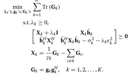
To demonstrate the tightness of SDR method we com-pute the rank one test (ROT) ratio defined as
ROT=max k
M
i=2λi(Gk) λ1(Gk)
,
where λi(Gk) denotes the i-th largest eigenvalue ofGk. The simulation result is shown in Figure 1 where each data point represents the maximum ROT ratio over 2000 Monte Carlo simulations. From this figure, we can see that the ROT ratio is very close to zero, suggesting that the solution of the SDR method is indeed always of rank one.
We also compare the SDR method with the convex restriction method proposed in [18]. Figure 2 presents the average transmission power versus the target SINR level, where each data point is averaged over 2000 Monte Carlo simulations. Note that, to guarantee the feasibility of the problem, we compare two methods only when the con-vex restriction method is feasible. From the figure, it can be observed that the SDR method is more power-efficient than the convex restriction method (which is abbreviated as ‘cvxRes’ in the figure).
Now we present three counter examples in which the uncertain bound does not satisfy inequalities (18) and the solution is not rank one accordingly. In the examples, we consider the channel uncertainty regions as (18). We set
σ12=σ22=σ32=1,
6 8 10 12 14 16
0 0.5 1 1.5 2 2.5x 10
−8
γ (dB)
Rank one test ratio
6 8 10 12 14 16 6
8 10 12 14 16 18 20 22
γ (dB)
Avergage transmission power (dB)
SDR cvxRes
Figure 2Average transmission power versus the target SINR.
B1= ⎡
⎣0.5 1 0.51 0.5 0 0 0.5 1
⎤ ⎦,B2=
⎡
⎣0.36 1.2 0.21 0.36 0.5 0.5 0.2 1
⎤
⎦ and
B3= ⎡
⎣0.4 1.5 01 0.4 0.2 0.2 0 1
⎤ ⎦
in (18).
Example 1. Three channel vectors are
˜ h1=
⎡
⎣−0.70630.9102−−1.00780.0127ii
−0.5121−0.9088i
⎤ ⎦,h˜2=
⎡
⎣−0.33120.8027−+0.72320.5017ii
−0.5206+0.5656i
⎤ ⎦
and h˜3= ⎡
⎣0.18590.4601−−0.10130.1435ii 0.2953+0.2650i
⎤ ⎦,
with SINR requirement γ1 = 0.8174, γ2 = 0.6475
and γ3 = 0.7893. and ellipsoid norm bound ¯ =
(0.5, 0.5, 0.46)T.
The solution of problem (P¯), G3 has eigenvalues
eig(G3)= ⎛
⎝355.9564−0.0000 669.2019
⎞ ⎠.
Our proposed rank one bound is
min ⎧ ⎨ ⎩¯3,
λmin(B3) γ3σ32
V(¯) ⎫ ⎬
⎭=0.0164
and Figure 3 reveals the rank distribution with respect to uncertain bound3when1= ¯1and1= ¯2.
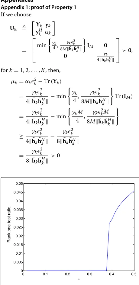
Example 2. Three channel vectors are
˜ h1=
⎡
⎣−−0.36010.4228+−0.14691.9893ii
−0.3266+0.5184i
⎤ ⎦,h˜2=
⎡
⎣−−0.56960.2249+−0.16230.3012ii
−0.7319−1.0981i
⎤ ⎦
and h˜3= ⎡
⎣−0.05880.0446−+0.93780.6998ii 0.3012+0.6243i
⎤ ⎦.
The SINR requirements are the same as previous exam-ple and ellipsoid norm bound is¯ = (0.5, 0.5, 0.46)T. The solution of problem (P¯), G3 has eigenvalues eig(G3) = ⎛
⎝277.92813.9948 374.1312
⎞
⎠. Our proposed rank one bound is
min ⎧ ⎨ ⎩¯3,
λmin(B3) γ3σ32
V(¯) ⎫ ⎬
⎭=0.020
and Figure 4 reveals the rank distribution with respect to uncertain bound3when1= ¯1and1= ¯2.
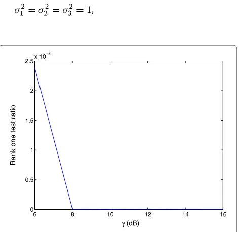
Example 3. Three channel vectors are
˜ h1=
⎡
⎣ 0.41081.2589+−0.10050.1619ii
−0.0924+0.4407i
⎤ ⎦,h˜2=
⎡
⎣−1.64000.9489++0.82440.5955ii
−0.2318+0.3206i
⎤ ⎦
and h˜3= ⎡
⎣0.38180.6173−+0.34270.9305ii 0.1524−0.2440i
⎤ ⎦,
0 0.05 0.1 0.15 0.2 0.25 0.3 0.35 0.4 0.45 0
0.1 0.2 0.3 0.4 0.5 0.6
ε
Rank one test ratio
0.2 0.4 0.6 0.8 1 0
0.1 0.2 0.3 0.4 0.5 0.6 0.7 0.8 0.9
ε
Rank one test ratio
Figure 4ROT ratio ofG3versus the uncertain bound3.
with SINR requirementγ1 = 1.2174, γ2 = 0.6475and γ3=0.7893and ellipsoid norm bound¯ =(0.5, 0.5, 0.5)T.
The solution of problem (P¯), G3 has eigenvalues that
eig(G3)= ⎛ ⎝ 54.40
1184.1 ⎞
⎠. Our proposed rank one bound is
min ⎧ ⎨ ⎩¯3,
λmin(B3) γ3σ32
V(¯) ⎫ ⎬
⎭=0.0132
and Figure 5 illustrates the change in the rank with respect to the increase in the uncertainty bound3when1 = ¯1
and1= ¯2.
Remark 4. The above three examples show that there might not be rank one when uncertainty bound3is larger
than our proposed bound. It also indicates that all the solu-tions are of rank one when uncertain bound is less than or equal to our proposed bound. It can be seen from figures that our proposed rank one bound is conservative, which means that there might be a larger region of uncertainty bounds for which the solution still remains rank one. This suggests that the bound proposed in Theorem 1 might be improved using some other techniques. This is an interest-ing problem, which can motivate further research on the topic.
Conclusions
We have considered the robust beamforming design prob-lem (PR) for a MISO downlink channel in this article. Our work mainly focused on the existence of a rank-one solu-tion for the corresponding SDP relaxasolu-tion (P). It is shown that the problem (PR) can be solved globally by the SDR method as long as the size of channel estimation errors are sufficiently small, or when the BS is equipped with two antennas. In addition, we have proved that when BS
is equipped with three antennas, for any solution(Gk,k= 1,. . .,K)of (P), there is at most oneGk with rank larger than one. The numerical experiments show that the SDR method gives better results in comparison with the exist-ing robust beamformexist-ing methods. Here, we just give a sufficient condition which guarantees that SDP relaxation (P) is tight. In fact, our numerical results show all the solutions of SDP relaxation (][]P) give rank one solutions when the uncertainty regions are balls, regardless of the size of the uncertainty bounds. On the other hand, we pro-vided examples to show that SDP relaxation may not be tight when the uncertainty regions are ellipsoids.
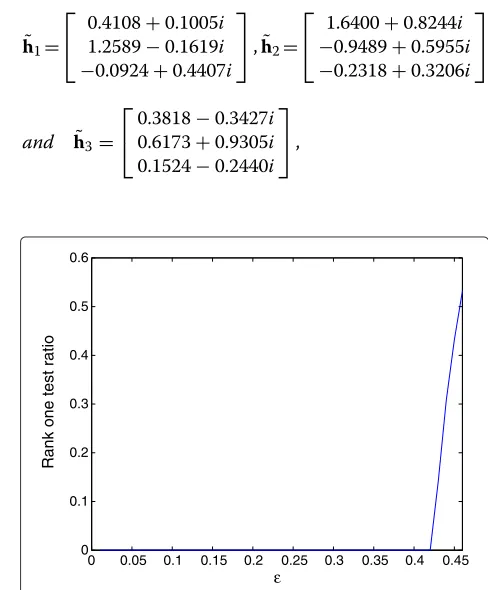
Appendices
Appendix 1: proof of Property 1
If we choose
Uk
Yk yk yHk αk
= ⎡ ⎢ ⎣min
γk
4, γkk2 8M˜hkh˜Hk
IM 0
0 γk
4˜hkh˜Hk ⎤ ⎥ ⎦0,
fork=1, 2,. . .,K, then,
μk=αkk2−Tr(Yk)
= γkk2 4˜hkh˜Hk
−min
' γk
4,
γk2k
8M˜hkh˜Hk (
Tr(IM)
= γkk2 4˜hkh˜Hk
−min
' γkM
4 ,
γk2kM
8M˜hkh˜Hk (
≥ γkk2 4˜hkh˜Hk
− γkk2 8˜hkh˜Hk
= γkk2 8˜hkh˜Hk
>0
0 0.1 0.2 0.3 0.4 0.5 0
0.005 0.01 0.015 0.02 0.025 0.03 0.035 0.04 0.045 0.05
ε
Rank one test ratio
and
which implies that {Uk} is a strictly feasible point of problem (D).
Appendix 2: proof of Lemma 3
in this section we prove Lemma 3.
Proof.Due to strong duality assumption, suppose λk’s, Gk’s,Yk’s,yk’s,αk’s are any primal and dual optimal points with zero duality gap.
Firstly, ifZkis positive definite, then we can increaseαk a little without violating any constraints. Hence, noZk’s is of full rank, which implies
rank(Zk)≤M−1. (20)
Secondly, we prove that
Zk =0, k=1, 2,. . .,K, (21)
which contradicts the fact that Zj cannot be full rank. Therefore, (21) holds true. Consequently,
rank(Zk)≥1, (24)
Thus, (11) is proved according to (20) and (24). Thirdly, we prove that
Gk=0, k=1, 2,. . .,K, (25)
by contradiction. AssumeGk=0, then we have
Xk =
which contradicts the fact
Since we assume the strong duality holds, then, by com-plementarity conditions, we have
Tr(GkZk)=0, (29)
which means that
rank(Gk)+rank(Zk)≤M. (30)
Competing interests
The authors declare that they have no competing interests.
Acknowledgements
This work was supported in part by the Army Research Office, grant number W911NF-09-1-0279, in part by the National Science Foundation, grant number DMS-1015346, and in part by the National Science Foundation of China, grant number 60901037. This work was completed during a visit of the first two authors to the University of Minnesota.
Author details
1Department of Mathematics, Sichuan University, Chengdu, Sichuan 610064,
China.2School of Information and Science Technology, Zhejiang Sci-Tech University, Hangzhou 310018, China.3Department of Electrical and Computer Engineering, University of Minnesota, Twin Cities, MN 55455, USA.
Received: 16 February 2012 Accepted: 11 July 2012 Published: 6 August 2012
References
1. M Bengtsson, B Ottersten, Optimal and Suboptimal Transmit Beamforming, Chapter 18. inHandbook of Antennas in Wireless Communications, ed. by LC Godara (CRC Press, New York, 2002) 2. H Boche, M Schubert, A general duality theory for uplink and downlink
beamforming. inProc. IEEE VTC-Fall(Vancouver, British Columbia, Canada, 2002)
3. AB Gershman, ND Sidiropoulos, S Shahbazpanahi, M Bengtsson, B Ottersten, Convex optimization-based beamforming. IEEE Signal Process. Mag.27, 62–75 (2010)
4. A Wiesel, YC Eldar, S Shamai, Linear precoding via conic optimization for fixed MIMO receivers. IEEE Trans. Signal Process.54(1), 161–176 (2006) 5. B Hassibi, BM Hochwald, How much training is needed in
multiple-antenna wireless links? IEEE Trans. Inf. Theory Process.49(4), 951–963 (2003)
6. DJ Love, Jr. Health RW, W Santipach, ML Honing, What is the value of limited feedback for MIMO channels? IEEE Commun. Mag.42, 54–59 (2004)
7. G J ¨ongren, M Skolgund, B Ottersten, Combining beamforming and orthogonal space-time block coding. IEEE Trans. Inf. Theory.48(3), 611–627 (2002)
8. T Weber, A Sklavos, M Meurer, Imperfect channel-state information in MIMO transmission. IEEE Trans. Commun.54(3), 543–552 (2006) 9. Y Rong, SA Vorobyov, AB Gershman, Robust linear receivers for
multi-access space-time block coded MIMO systems: a probabilistically constrained approach. IEEE J. Sel. Areas Commun.24(8), 1560–1570 (2006) 10. M Botros Shenouda, TN Davidson, On the design of linear transceivers for
multiuser systems with channel uncertainty. IEEE J. Sel. Areas Commun. 26(6), 1015–1024 (2008)
11. X Zhang, DP Palomar, B Ottersten, Statistically robust design of linear MIMO transceivers. IEEE Trans. Signal Process.56(8), 3678–3689 (2008) 12. MB Shenouda, TN Davidson, Probabilistically-constrained approaches to
the design of the multiple antenna downlink. inProc. IEEE Asilomar Conf. Signals, Systems and Computers(Pacific Grove, 26–29 Oct 2008), pp. 1120–1124
13. N Vuˇci´c, H Boche, a tractable method for chance-constrained power control in downlink multiuser MISO systems with channel uncertainty. IEEE Signal Process. Lett.16(5), 346–349 (2009)
14. SA Kassam, HV Poor, Robust techniques for signal processing: a survey. Proc. IEEE.73(3), 433–482 (1985)
15. SA Vorobyov, AB Gershman, Z-Q Luo, Robust adaptive beamforming using worst-case performance optimization: a solution to the signal mismatch problem. IEEE Trans. Signal Process.51(2), 313–324 16. A Mutapcic, S-J Kim, S Boyd, A tractable method for robust downlink
beamforming in wireless communications. inProc. IEEE Asilomar Conf. Signals, Systems and Computers(Pacific Grove, CA, USA, 4–7 Nov 2007), pp. 1224–1228
17. A Abdel-Samad, TN Davidson, AB Gershman, Robust transmit eigen beamforming based on imperfect channel state information. Trans. Signal Process.54(5), 1596–1609 (2006)
18. N Vuˇci´c, H Boche, Robust QoS-constrained optimization of downlink multiuser MISO systems. IEEE Trans. Signal Process.57(2),
714–725 (2009)
19. MB Shenouda, TN Davidson, Convex conic formulations of robust downlink precoder designs with quality of service constraints. IEEE J. Sel. Topics Signal Process.1, 714–724 (2007)
20. G Zheng, K-K Wong, T-S Ng, Robust linear MIMO in the downlink: a worst-case optimization with ellipsoidal uncertainty regions. EURASIP J. Adv. Signal Process.2008, 1–15 (2008)
21. Z-Q Luo, W-K Ma, AM-C So, Y Ye, S Zhang, Semidefinite relaxation of quadratic optimization problems. IEEE Signal Process. Mag.27, 20–34 (2010)
22. Z-Q Luo, T-H Chang, SDP Relaxation of Homogeneous Quadratic Optimization: Approximation Bounds and Applications, Chapter 4. in Convex Optimization in Signal Processing and Communications, ed. by DP Palomar and Y Eldar (Cambridge University, UK, 2010)
23. S Boyd, L Vandenberghe,Convex Optimization(Cambridge University Press, Cambridge, UK, 2004)
24. S Boyd, L El Ghaoui, E Feron, V Balakrishnan,Linear Matrix Inequalities in System and Control Theory(SIAM, Philadelphia, PA, 1994)
doi:10.1186/1687-1499-2012-243
Cite this article as:Songet al.:Robust SINR-constrained MISO downlink beamforming: when is semidefinite programming relaxation tight?. EURASIP Journal on Wireless Communications and Networking20122012:243.
Submit your manuscript to a
journal and benefi t from:
7Convenient online submission
7Rigorous peer review
7Immediate publication on acceptance
7Open access: articles freely available online
7High visibility within the fi eld
7Retaining the copyright to your article