Hopf bifurcation analysis in a predator–prey model with two time delays and stage structure for the prey

R E S E A R C H

Open Access

Hopf bifurcation analysis in a

predator–prey model with two time delays

and stage structure for the prey

Miao Peng

_{and Zhengdi Zhang}

*_{Correspondence:}

[email protected]

1_{Faculty of Science, Jiangsu}

University, Zhenjiang, P.R. China

Abstract

In this paper, a stage-structured predator–prey model with Holling type III functional response and two time delays is investigated. By analyzing the associated

characteristic equation, its local stability and the existence of Hopf bifurcation with respect to both delays are studied. Based on the normal form method and center manifold theorem, the explicit formulas are derived to determine the direction of Hopf bifurcation and the stability of bifurcating period solutions. Finally, the effectiveness of theoretical analysis is verified via numerical simulations. This study may be helpful in understanding the behavior of ecological environment.

Keywords: Hopf bifurcation; Predator–prey model; Time delay; Stage structure; Local stability

1 Introduction

The dynamics of predator–prey models is one of important subjects in ecology and math-ematical ecology, and many factors, such as time delay, disease, harvesting, functional re-sponse, etc., can affect it in the natural world.

In recent years, some researchers have discussed predator–prey models with these fac-tors. Wangersky and Cunningham [1] considered a predator–prey system with time delay and studied the effect of time delay on the system. May [2] also analyzed the stability of vegetation–herbivore and vegetation–herbivore–carnivore systems with time delay. They found that a model with time delay could cause a stable equilibrium to become unsta-ble and cause the population to fluctuate. Hu and Li [3] described a mathematical model dealing with a predator–prey system with disease in the prey, they discussed the prop-erties of Hopf bifurcation. Banshidhar and Swarup [4] proposed a predator–prey model with harvesting where the top predator population is partially supported with alternative food. Their research showed that alternative food can prevent top predator extinction risk at higher harvesting effort. Yang [5] discussed the stability in a delayed diffusive predator– prey model with nonconstant death rate. Zhu et al. [6] studied a predator–prey model with time delay and square root response function. As we all know, non-smooth factor is used in mechanical engineering [7,8]. In fact, non-smooth factor is also found in a predator– prey model. Chen and Huang [9] investigated a Filippov ratio-dependent predator–prey model to describe the effect on behavioral refuges caused by prey instinct anti-predator

behavior. They discussed complete analysis of local and global dynamical behaviors of this model by Filippov qualitative theory. Peng et al. [10] proposed a hybrid control strategy in a predator–prey model. Their numerical simulation results showed that the hybrid con-troller is efficient in controlling a Hopf bifurcation.

In nature, there are many species whose individuals have a life history that can be di-vided into two stages: immature and mature. The stage structure reflects the species’ ac-tivity ability and the difference about resistance to natural enemies in different growth period. It can affect the persistence and extinction of biological populations to various de-gree. Therefore, it is more practical to discuss the predator–prey model with this factor. Meng et al. [11] studied the stability and Hopf bifurcation in a three-species system with stage structure for the predator. Ref. [12,13] also have paid great attention to discussing the effect with stage structure in predator–prey models. In [14], Wang et al. considered a delayed ratio-dependent predator–prey system with Holling type III functional response and stage structure for the predator:

˙

x(t) =x(t)

r–ax(t–τ1) –

a1x(t)y2(t)

my22(t) +x2(t)

,

˙

y1(t) =

a2x2(t–τ2)y2(t–τ2)

my2₂(t–τ2) +x2(t–τ2)

–r1y1(t) –Dy1(t),

˙

y2(t) =Dy1(t) –r2y2(t),

(1.1)

wherex(t) represents the density of the prey population at timet,y1(t) andy2(t) describe

the densities of the immature and the mature predator population at timet, respectively. The parametersr,a,a1,a2,m,r1,r2, andDare positive constants in whichrrepresents

the intrinsic growth rate of the prey, ais the intraspecific competition rate of the prey,

a1is the capturing rate,a2/a1is the conversion rate of the mature predator,mis the half

capturing saturation constant,r1andr2are the death rates of the immature and the

ma-ture predator, respectively.Ddenotes the rate at which the immature predator becomes the mature predator.τ1is the feedback time delay of the prey,τ2is the time delay due to

the gestation of the mature predator. In [14], Wang et al. investigated the local stability of each of the feasible equilibria of the system and the related properties of Hopf bifurca-tion.

However, some predator species dislike hunting immature preys, or many immature preys are concealed in the caves or nests to keep from being attacked by the predators in the natural world. In this paper, based on the above discussions and motivated by the work of Wang et al. [14], we consider the following system with stage structure for the prey and two delays:

˙

x1(t) =ax2(t) –bx1(t) –r1x1(t) –cx1(t)x1(t–τ1) –

a1x21(t)y(t)

1 +mx2 1(t)

,

˙

x2(t) =bx1(t) –r2x2(t),

˙

y(t) =a2x

2

1(t–τ2)y(t–τ2)

1 +mx2 1(t–τ2)

–ry(t),

(1.2)

wherex1(t),x2(t) describe the densities of the immature prey and the mature prey at time

the immature prey, bis the transformation rate from the immature prey to the mature one,cis the intraspecific competition coefficient of the immature prey,r1,r2,rdenote the

death rates of immature prey, mature prey, and predator.a2/a1 is the conversion rate of

the predator,τ1is the feedback time delay of the immature prey, andτ2is the time delay

due to the gestation of the predator. The rest of parametersa1,mare similar to those of

model (1.1).

The organization of this paper is as follows. In Sect.2, the local stability of the positive equilibrium and the existence of Hopf bifurcation for system (1.2) are studied. The direc-tion of Hopf bifurcadirec-tion and the stability of bifurcating periodic soludirec-tions are derived in Sect.3. In Sect.4, numerical simulations are carried out to illustrate the validity of the established results. Finally, a brief conclusion is given.

2 Local stability and Hopf bifurcation

From the viewpoint of biology, we only study the positive equilibrium of system (1.2). In this section, we shall discuss the local stability of a linearized system at the positive equilibrium and the existence of Hopf bifurcations for system (1.2).

It is easy to show that system (1.2) has a unique positive equilibrium E∗(x₁∗,x∗₂,y∗), where

x∗₁=

r a2–rm

,

x∗₂= b

r2

x∗₁,

y∗=(ab–r1r2–br2–cr2x

∗

1)(1 +mx∗21 )

a1r2x∗1

if the following conditions are satisfied:

(H1) a2–rm> 0, ab–r1r2–br2–cr2

r a2–rm

> 0.

Letx¯1(t) =x1(t) –x∗1,x¯2(t) =x2(t) –x∗2,y¯(t) =y(t) –y∗and still denotex¯1(t),x¯2(t),y¯(t),

respectively. Using Taylor’s expansion to expand system (1.2) at the positive equilibrium

E∗(x∗₁,x∗₂,y∗), we have

˙

x1(t) =a11x1(t) +a12x2(t) +a13y(t) +b11x(t–τ1)

+

i+j+k+q≥2

f₁(ijkq)xi₁(t)xj₂(t)ykxq₁(t–τ1),

˙

x2(t) =a21x1(t) +a22x2(t) +

i+j≥2

f₂(ij)xi₁(t)xj₂(t),

˙

y(t) =b31x1(t–τ2) +a33y(t) +b33y(t–τ2) +

i+j+k≥2

f₃(ijk)yi(t)xj₁(t–τ2)yk(t–τ2),

where

Then we obtain the linearized system of system (2.1) as follows:

˙

Therefore, the corresponding characteristic equation of system (2.2) is given by

λ3+m2λ2+m1λ+m0+

Lemma 2.1 For the transcendental equation

pλ,e–λτ1_{, . . . ,e}–λτm_=λn_+p(0)

1 λn–1+· · ·+p (0) n–1λ+p(0)n

+ p(1)₁ λn–1+· · ·+p(1)_n–1λ+p(1)_n e–λτ1₊· · ·

+ p(m)₁ λn–1+· · ·+p_n–1(m)λ+p(m)_n e–λτm

= 0,

as(τ1,τ2,τ3, . . . ,τm)vary,the sum of orders of the zeros of p(λ,e–λτ1, . . . ,e–λτm)in the open

right half plane can change,and only a zero appears on or crosses the imaginary axis.

Next, we will consider the following four cases.

Case 1:τ1=τ2= 0, the characteristic Eq. (2.3) reduces to

λ3+m12λ2+m11λ+m10= 0, (2.4)

wherem10=m0+n0+p0+q0,m11=m1+n1+p1,m12=m2+n2+p2.

It is not difficult to verify thatm10 > 0,m12> 0. Thus, all the roots of Eq. (2.4) have

negative real parts if the following condition holds:

(H11) m11m12>m10.

Namely, the equilibrium pointE∗(x∗₁,x∗₂,y∗) is locally asymptotically stable when condition (H11) is satisfied.

Case 2:τ1= 0,τ2> 0. Equation (2.3) becomes

λ3+m22λ2+m21λ+m20+

p22λ2+p21λ+p20

e–λτ2_{= 0, (2.5)}

wherem20=m0+n0,m21=m1+n1,m22=m2+n2,p20=p0+q0,p21=p1+q1,p22=p2.

Letiω2(ω2> 0) be a root of Eq. (2.5), it follows that

p21ω2sinω2τ2+

p20–p22ω22

cosω2τ2=m22ω22–m20,

p21ω2cosω2τ2–

p20–p21ω22

sinω2τ2=ω23–m21ω2,

(2.6)

which leads to

ω6₂+e22ω42+e21ω22+e20= 0, (2.7)

wheree20=m220–p220,e21=m221– 2m20m22–p221+ 2p20p22,e22=m222– 2m21–p222.

Letω₂2=v2, then Eq. (2.7) can be written as

v3₂+e22v22+e21v2+e20= 0. (2.8)

Denote

Sincef1(0) =e20,limv2→+∞f1(v2) = +∞, and from Eq. (2.9), we have

f₁(v2) = 3v22+ 2e22v2+e21. (2.10)

After discussion about the roots of Eq. (2.10) similar to that in [16], we have the following lemma.

Lemma 2.2 For the polynomial Eq. (2.8),we have the following results: (1) If

(H21) e20≥0, =e222– 3e21≤0 holds,then Eq. (2.8)has no positive root; (2) If

(H22) e20≥0, =e222 – 3e21> 0, v∗2=

–e21+ √

3 > 0, f1

v∗₂≤0,

or

(H23) e20< 0

holds,then Eq. (2.8)has a positive root.

Suppose that Eq. (2.8) has positive roots. Without loss of generality, we assume that it has three positive roots, which are denoted byv21,v22, andv23. Then Eq. (2.7) has three

positive rootsω2k=√v2k,k= 1, 2, 3. The corresponding critical value of time delayτ2k(j)is

τ_2k(j)= 1

ω2k arccos

A24ω2k4 +A22ω2k2 +A20

B24ω42k+B22ω22k+B20

+2πj

ω2k

, k= 1, 2, 3;j= 0, 1, 2, . . . , (2.11)

whereA20= –m20p20,A22=m22p20+m20p22–m21p21,A24=p21–m22p22,B20=p220,B22=

p2₂₁– 2p20p22,B24=p222.

Thus±ω2kis a pair of purely imaginary roots of Eq. (2.5) withτ2=τ2k(j), and letτ20= mink∈{1,2,3}{τ_2k(0)},ω20=ω2k0.

Lemma 2.3 Suppose that

(H24) f₁ω2₂₀= 0,

then the following transversality condition holds:

d(Reλ)

dτ2

λ=iω20

= 0.

Proof Differentiating Eq. (2.5) with respect toτ2, and noticing thatλis a function ofτ2,

we obtain

dλ

dτ2

–1

= – 3λ

2_{+ 2m}

22λ+m21

λ(λ3_+m

22λ2+m21λ+m20)

+ 2p22λ+p21

λ(p22λ2+p21λ+n20)

–τ1

which leads to

Letiω(ω> 0) be the root of Eq. (2.16), and separate the real and imaginary parts, we have

E31sinωτ+E32cosωτ=E35,

E33cosωτ+E34sinωτ=E36,

(2.17)

whereE31= –m31ω+ω3+q31ω,E32=m30–m32ω2+q30,

E33=m31ω–ω3+q31ω, E34=m30–m32ω2–q30,

E35=n32ω2–n30, E36= –n31ω.

It follows that

sinωτ= A35ω

5_+A

33ω3+A31ω

ω6_+B

34ω4+B32ω2+B30

, cosωτ= A34ω

4_+A

32ω4+A30

ω6_+B

34ω4+B32ω2+B30

, (2.18)

where

A30= (q30–m30)n30, A31= (m31+q31)n30– (m30+q30)n31,

A32= (m30–q30)n32–m31n31+m32n30+q31n31,

A33=m32n31–n30–m31n32–q31n32,

A34=n31–m32n32, A35=n32, B30=m230–q302,

B32=m231–q231– 2m30m32, B34=m232– 2m31.

From Eq. (2.18), we get

ω12+e35ω10+e34ω8+e33ω6+e32ω4+e31ω2+e30= 0, (2.19)

where

e30=B230–A230, e31= 2B30B32–A231– 2A30A32,

e32=B232+ 2B30B34–A232– 2A30A34– 2A31A33,

e33= 2B30+ 2B32B34–A233– 2A31A35– 2A32A34,

e34=B234+ 2B32–A234– 2A33A35, e35= 2B34–A235.

Letω2_=v

3, then Eq. (2.19) can be written as

v6₃+e35v53+e34v43+e33v33+e32v23+e31v3+e30= 0. (2.20)

Suppose that Eq. (2.20) has at least one positive root, and without loss of generality, we assume that it has six positive roots which are denoted byv31,v32,v33,v34,v35,v36, then

value of time delayτ_k(j)is

holds,then the following transversality condition is satisfied:

Proof Differentiating Eq. (2.16) with respect toτ, we obtain

This completes the proof.

By applying Lemma2.4to Eq. (2.16), we obtain the existence of a Hopf bifurcation as stated in the following theorem.

Theorem 2.2 For system(1.2),τ1=τ2=τ= 0.Suppose that condition(H31)holds,then the

positive equilibrium E∗(x∗₁,x∗₂,y∗)is asymptotically stable for allτ∈[0,τ0)and unstable for

τ >τ0.Furthermore,system(1.2)undergoes a Hopf bifurcation at the positive equilibrium

Case 4:τ1> 0,τ2∈[0,τ20), andτ1=τ2.

We consider Eq. (2.3) withτ2in its stable interval, andτ1is regarded as the parameter.

Letiω1∗(ω1∗> 0) be the root of Eq. (2.3), then we obtain

E41sinω1∗τ1+E42cosω1∗τ1=E43,

E41cosω1∗τ1–E42sinω1∗τ1=E44,

(2.24)

where

E41=n1ω1∗–q0sinω1∗τ2+q1ω1∗cosω1∗τ2,

E42=n0–n2ω12∗+q0cosω1∗τ2+q1ω1∗sinω1∗τ,

E43=m2ω21∗–m0+

p2ω21∗–p0

cosω1∗τ2–p1ω1∗sinω1∗τ2,

E44=ω31∗–m1ω1∗–

p2ω21∗–p0

sinω1∗τ2–p1ω1∗cosω1∗τ2.

From Eq. (2.24), we have

ω6_1∗+e42ω41∗+e41ω21∗+e40+

c44ω41∗+c42ω12∗+c40

cosω1∗τ2

+c45ω51∗+c43ω31∗+c41ω1∗

sinω1∗τ2= 0, (2.25)

where

e40=m20+p20–n02–q02, e41=m21+p21–n21–q21+ 2n0n2– 2m0m2– 2p0p2,

e42=m22–n22– 2m1+p22, c40= 2m0p0– 2n0q0,

c41= 2p1m0– 2p0m1+ 2n1q0– 2n0q1,

c42= 2p1m1– 2p0m2+ 2n2q0– 2p2m0– 2n1q1,

c43= 2p0– 2p1m2+ 2p2m1+ 2n2q1, c44= –2p1+ 2p2m2, c45= –2p2.

In order to give the main results, we provide the following assumption.

(H41) Eq. (2.25) has at least a finite positive root.

We denote the positive roots of Eq. (2.25) byω(1)_1∗,ω(2)_1∗,ω₁(3)_∗,ω₁(4)_∗,ω(5)_1∗, andω(6)_1∗. For every

ω(i)_1∗(i= 1, 2, 3, 4, 5, 6), the corresponding critical value of time delayτ_1i(j),j= 1, 2, 3 . . . , is

τ_1i(j)= 1

ω1∗

arccos

E41E44+E42E43

E2 41+E422

+ 2πj

ω1∗=ωi_1∗ ,

i= 1, 2, 3, 4, 5, 6;j= 0, 1, 2 . . . . (2.26)

Letτ₁₀ =min{τ_1i(0)|i= 1, 2, . . . 6;j= 0, 1, 2 . . .},ω₁₀is the corresponding root of Eq. (2.25) withτ₁₀ .

Lemma 2.5 Suppose that

holds,then the following transversality condition holds:

Obviously, if condition (H42) holds, then we have{d(Re_dτλ)

1 }λ=iω10 = 0. This completes the

proof of the lemma.

By the above analysis, we have the following theorem.

Theorem 2.3 For system(1.2),τ1> 0,τ2∈[0,τ20),andτ1=τ2.Suppose that conditions

(H41)and(H42)hold,then the positive equilibrium E∗(x₁∗,x∗₂,y∗)is asymptotically stable for allτ1∈[0,τ10 )and unstable forτ1>τ10 .Furthermore,system(1.2)undergoes a Hopf

bifurcation at the positive equilibrium E∗(x∗₁,x∗₂,y∗)whenτ1=τ10 .

3 Direction and stability of Hopf bifurcation

In the previous section, we have shown that system (1.2) undergoes a Hopf bifurcation for different combinations ofτ1 andτ2. In this section, we shall study the direction of Hopf

bifurcation and the stability of bifurcating periodic solutions of system (1.2) with respect to

τ1andτ2∈[0,τ20). The theoretical approach we apply is based on the normal form theory

Without loss of generality, we assume that τ₁₀ >τ₂. Letτ1=τ10 +μ, μ∈R, t=sτ1,

Hence, by the Riesz representation theorem, there exists a 3×3 matrix functionη(θ,μ) of bounded variation forθ∈[–1, 0] such that

Lμφ=

0

–1

In fact, we can choose

Then Eq. (3.1) can be transformed into the following operator equation:

u_t=A(μ)ut+R(μ)ut. (3.8)

Forϕ∈C([–1, 0], (R3₎∗_{), where (R}3₎∗ _{is the three-dimensional space of row vectors, we}

further define the adjoint operatorA∗ofA(0):

A∗ϕ(s) =

10τ10 θ _{is the eigenvector of A(0) corresponding to}

iω₁₀τ₁₀ andq∗(s) = 1/ρ(1,q₂∗,q₃∗)eiω10τ10 s_{is the eigenvector ofA}∗_{corresponding to –iω}

10τ10 .

By the direct calculation, we obtain

Then, from Eq. (3.10), we get

In the remainder of this section, by using the algorithms in [18] and using a similar calcu-lation process to that in [10], we obtain the coefficients used in determining the direction of Hopf bifurcation and the stability of the bifurcation periodic solutions:

whereE1= (E(1)1 ,E

and can be determined by the following equations, respectively:

⎛

Therefore, we can calculateg21and compute the following values:

c1(0) =

which determine the properties of bifurcating periodic solutions atτ=τ₁₀ on the center manifold. From the discussion above, we have the following result.

Theorem 3.1 For system(1.2),the direction of Hopf bifurcation is determined by the sign ofμ2:ifμ2> 0 (μ2< 0),then the Hopf bifurcation is supercritical(subcritical).The stability

of the bifurcating periodic solutions is determined by the sign ofβ2:ifβ2< 0 (β2> 0),the

bifurcating periodic solutions are stable(unstable).The period of the bifurcating periodic solutions is determined by the sign of T2:if T2> 0 (T2< 0),the bifurcating periodic solutions

4 Numerical examples

In this section, we give some numerical simulations by using matlab to illustrate the ana-lytical results in the previous section.

Leta= 8,b= 1,c= 1,a1= 3,r1= 0.5,a2= 2,r2=r= 1,m= 1. Then we have the following

particular example of system (1.2):

˙

x1(t) = 8x2(t) – 0.5x1(t) –x1(t) –x1(t)x1(t–τ1) –

3x2 1(t)y(t)

1 +x2 1(t)

,

˙

x2(t) =x1(t) –x2(t),

˙

y(t) =2x

2

1(t–τ2)y(t–τ2)

1 +x2 1(t–τ2)

–y(t).

(4.1)

It is not difficult to verify that condition (H1) holds, we obtain the positive equilibrium

E∗(1, 1,11₃).

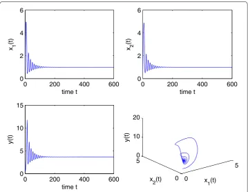
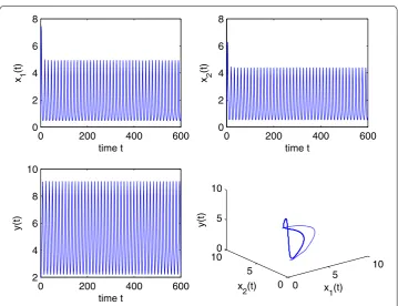
Forτ1= 0,τ2> 0, we obtainw20≈0.4609,τ20≈1.9387. From Theorem2.1, we know that

the positive equilibriumE∗is asymptotically stable whenτ2∈[0,τ20), when the time delay

τ2passes through the critical valueτ20, the interior equilibriumE∗will lose its stability and

a Hopf bifurcation occurs, and a family of periodic solutions bifurcate from the interior equilibriumE∗. The corresponding waveform and the phase plots are depicted in Fig.1 and Fig.2.

Forτ1=τ2=τ, we getω0= 0.5385,τ0= 1.7889. By Theorem2.2, we know that, when

τ increases from zero to the critical valueτ0, the equilibrium pointE∗is asymptotically

stable. Once the time delayτpasses through the critical valueτ0, the positive equilibrium

Figure 2Whenτ1= 0,E∗undergoes a Hopf bifurcation forτ2= 1.98 >τ20= 1.9387

E∗will lose its stability and a Hopf bifurcation occurs, which can be depicted in Fig.3and Fig.4.

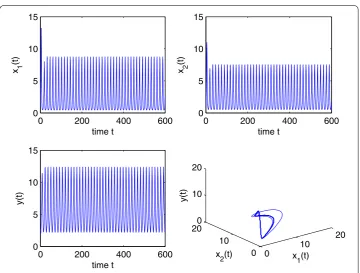
Forτ1> 0,τ2= 1.5∈[0,τ20), we haveω10= 0.5974,τ10 = 2.3522. According to

Theo-rem 2.3, E∗ is asymptotically stable when τ1∈[0,τ10 ) and unstable whenτ1>τ10 .

Af-ter the computation of Eq. (3.17), we obtainc1(0) = –22.3543 + 6.0903i,μ2= 444.4195,

β2= –44.7086,T2= –11.6715. From Theorem3.1, the Hopf bifurcation is supercritical,

the bifurcating periodic solutions are stable, which is shown in Fig.5and Fig.6.

Numerical simulations illustrate our theoretical analysis. Owing to the bifurcation peri-odic solutions being stable, the species in system (1.2) can coexist in an oscillatory mode from the viewpoint of biology.

5 Conclusions

cer-Figure 3Whenτ1=τ2=τ,E∗is asymptotically stable forτ= 1.1 <τ0= 1.7889

Figure 5 E∗is asymptotically stable forτ1= 1.4 <τ10 = 2.3522 andτ2= 1.5

tain ecological significance and provides a powerful theoretical basis for the sustainable survival of natural populations.

In addition, stage structure for the prey is investigated in this paper due to the predator feeding only on the immature prey. If we were concerned with the combined effects of stage structure for both the predator and the prey, what will the dynamical behavior of the system be? This issue is left as our future research.

Acknowledgements

The authors would like to thank the referees for the careful reading of the manuscript and valuable suggestions.

Funding

This work was supported by the National Natural Science Foundation of China (No. 11472116), the Key Program of the National Natural Science Foundation of China (No. 11632008), and Postgraduate Research & Practice Innovation Program of Jiangsu Province (KYCX17_1784).

Competing interests

The authors declare that they have no competing interests.

Authors’ contributions

All authors contributed equally to the writing of this paper. The authors read and approved the final manuscript.

Publisher’s Note

Springer Nature remains neutral with regard to jurisdictional claims in published maps and institutional affiliations.

Received: 21 February 2018 Accepted: 8 July 2018

References

1. Wangersky, P.J., Cunningham, W.J.: Time lag in prey–predator population models. Ecology38(1), 136–139 (1957) 2. May, R.M.: Time delay versus stability in population models with two and three trophic levels. Ecology54(2), 315–325

(1973)

3. Hu, G.P., Li, X.L.: Stability and Hopf bifurcation for a delayed predator–prey model with disease in the prey. Chaos Solitons Fractals45(3), 229–237 (2012)

4. Banshidhar, S., Swarup, P.: Effects of supplying alternative food in a predator–prey model with harvesting. Appl. Math. Comput.234, 150–166 (2014)

5. Yang, R.Z.: Hopf bifurcation analysis of a delayed diffusive predator–prey system with nonconstant death rate. Chaos Solitons Fractals81(6), 224–232 (2015)

6. Zhu, X.Y., Dai, Y.X., Li, Q.L., Zhao, K.H.: Stability and Hopf bifurcation of a modified predator-prey model with a time delay and square root response function. Adv. Differ. Equ.2017, 235 (2017).

https://doi.org/10.1186/s13662-017-1292-1

7. Li, X.H., Hou, J.Y.: Bursting phenomenon in a piecewise mechanical system with parameter perturbation in stiffness. Int. J. Non-Linear Mech.81, 165–176 (2016)

8. Li, X.H., Hou, J.Y., Chen, J.F.: An analytical method for Mathieu oscillator based on method of variation of parameter. Commun. Nonlinear Sci. Numer. Simul.37, 326–353 (2016)

9. Chen, X.Y., Huang, L.H.: A Filippov system describing the effect of prey refuge use on a ratio-dependent predator–prey model. J. Math. Anal. Appl.428(2), 817–837 (2015)

10. Peng, M., Zhang, Z.D., Wang, X.D.: Hybrid control of Hopf bifurcation in a Lotka–Volterra predator-prey model with two delays. Adv. Differ. Equ.2017, 387 (2017).https://doi.org/10.1186/s13662-017-1434-5

11. Meng, X.Y., Huo, H.F., Zhang, X.B., Xiang, H.: Stability and Hopf bifurcation in a three-species system with feedback delays. Nonlinear Dyn.64(4), 349–364 (2011)

12. Boonrangsiman, S., Bunwong, K., Moore, E.J.: A bifurcation path to chaos in a time-delay fisheries predator–prey model with prey consumption by immature and mature predators. Math. Comput. Simul.124, 16–29 (2016) 13. Khajanchi, S.: Modeling the dynamics of stage-structure predator–prey system with Monod–Haldane type response

function. Appl. Math. Comput.302, 122–143 (2017)

14. Wang, X.D., Peng, M., Liu, X.Y.: Stability and Hopf bifurcation analysis of a ratio-dependent predator–prey model with two time delays and Holling type III functional response. Appl. Math. Comput.268, 496–508 (2015)

15. Ruan, S., Wei, J.: On the zero of some transcendental functions with applications to stability of delay differential equations with two delays. Dyn. Contin. Discrete Impuls. Syst., Ser. A Math. Anal.10(6), 863–874 (2003)

16. Song, Y., Wei, J.: Bifurcation analysis for Chen’s system with delayed feedback and its application to control of chaos. Chaos Solitons Fractals22(1), 75–91 (2004)

17. Hale, J.K.: Theory of Functional Differential Equations. Springer, New York (1977)

18. Hassard, B.D., Kazarinoff, N.D., Wan, Y.H.: Theory and Application of Hopf Bifurcation. Cambridge University Press, Cambridge (1981)