ISSN 2348 – 7968
633
Brain Abnormality Detection in MRI Images based on Estimation of
Statistical Texture Measures
Namratha D’cruz1, Sudheesh.K.V2
1 Vidyavardhaka College of Engineering, Department of EC,
Mysuru, Karnataka, India
2 Vidyavardhaka College of Engineering, Department of EC,
Mysuru, Karnataka, India
Abstract
The field of radiology is rapidly evolving with the recent advancements in imaging techniques. MRI is the most commonly used imaging technique to detect and automatically classify abnormalities in human brain and this process is most challenging and time consuming. In this paper an automatic method to detect the abnormalities in brain MRI is proposed. It consists of 3 phases: Skull Stripping, Feature Extraction and Classification. In the initial phase skull region is removed using morphological operations. In the next phase texture features are extracted and in the last phase classification between normal and abnormal slices is done using SVM classifier. Software used is MATLAB R2014a.
Keywords: Radiology, Imaging Techniques, Skull Stripping, Texture Features, SVM classifier.
1. Introduction
Now a day’s computer technology is widely used in the field of medicine. Various imaging techniques are used to diagnose abnormalities in the patients noninvasively and without human intervention. Medical image analysis and preprocessing plays a very important role in the diagnosis and analysis of abnormalities by the doctors and radiologists. Different methods of obtaining medical images include X ray, Computed Tomography (CT) and Ultrasound. In recent day’s mammography, Magnetic Resonance Imaging (MRI), Positron Emission Tomography (PET), Single Photon Emission Computed Tomography (SPECT) and fusion of images from different modalities are used for better analysis and accurate diagnosis.
Magnetic Resonance Imaging (MRI) is most commonly used for diagnosis of abnormalities in brain because of the advantages like clear differentiation of soft tissues, noninvasive, high spatial resolution and contrast. MRI uses magnetic field and radio waves to produce high quality 2D and 3D images. These images are analyzed by radiologists to diagnose abnormalities present. The data’s are often large and analysis of such large data set are time consuming and prone to error. Therefore it is necessary to
have an automatic system to diagnose the abnormalities as it deals with precious human life[1].
There are two approaches for classification. The first approach is supervised learning approach where Artificial Neural Network (ANN), Support Vector Machine (SVM) and K-Nearest Neighbor (KNN) are used and the second approach is unsupervised learning approach for data clustering like Self Organizing Map (SOM) and K-means Clustering (KNN)[2]. In this paper supervised learning approach i.e. Support Vector Machine (SVM) is used as it gives better classification accuracy and performance.
2. Methodology
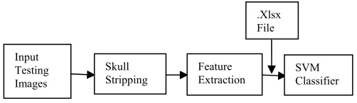
The proposed method is as shown in Fig 1. and Fig 2. It consists of three stages Skull Stripping, Feature Extraction and Classification.
Fig. 1: Block Diagram for Training SVM Classifier.
In the first stage MRI images are processed to remove the noise present in the image and further skull region is removed using morphological operations. In the second stage GLCM matrix of the image is calculated and different texture features are extracted from the matrix.
Fig. 2: Block Diagram for Testing SVM Classifier. Input
Training Images
Skull Stripping
Feature
Extraction Save as .xlsx
.Xlsx File
Input Testing Images
Skull Stripping
Feature
ISSN 2348 – 7968
634 In the third stage the extracted features are given as input
to the SVM classifier for training and testing.
2.1 Database
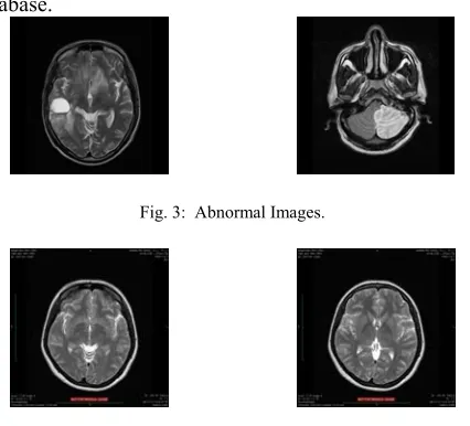
In this work the database consists of 2 sets i.e. for training and testing. T2 weighted real time brain MRI images collected from MRI scanning center are considered in this work. T2 weighted images are used as most of the abnormalities can be accurately identified. Total 70 images are taken. 40 images are used for training SVM classifier out of which 20 are normal and 20 are abnormal. Remaining 30 images are used for testing where 15 are normal and 15 are abnormal images. Fig 3 and Fig 4 shows some of the T2 weighted images taken for the database.
Fig. 3: Abnormal Images.
Fig. 4: Normal Images.
3. Skull Stripping
MRI images contains patient label (Film Artifacts), noise like salt and pepper noise and skull regions. Therefore it cannot be used directly without preprocessing as it affects the accuracy of the classification. Median Filtering is used to remove Film Artifacts and noise from the image and further the skull region is removed using mathematical morphology[3]. The algorithm for skull stripping is as follows:
3.1 Algorithm for Skull Stripping
1. Input MRI image.
2. Convert the RGB image to Gray Scale image.
3. Remove the noise and artifacts present in the image using Median Filter with suitable mask.
4. Choose square shaped structuring element.
5. Apply erosion operation 3 times by changing the size of the structuring element.
6. The image obtained after step 5 is the image without skull region.
4. Feature Extraction
Feature Extraction is a process of representing the image in an alternate way by measuring certain properties of the image that distinguishes one image from the other. One of the major problems that arise in the analysis of large data is the large number of variables. Large number of variables requires more memory and computation power thereby making analysis complex and inefficient. Therefore good features have to be extracted in order to make analysis easier and accurate. Most of the abnormal tissues are heterogeneous tissues and the mean values of relaxation times are not at all sufficient to characterize the heterogeneity of the different abnormality. An alternative approach is to apply texture analysis to the T2 images to describe quantitatively the brightness and texture of the images. Texture features represent the underlying characteristics of textures in unique and simpler way. It plays a very important role in image analysis and pattern recognition[4]. In this paper first order and second order texture features are calculated. The best method of extracting second order texture features are by using Gray Level Co-Occurrence Matrix (GLCM). From GLCM matrix different second order texture features are extracted.
4.1 Extraction of GLCM
ISSN 2348 – 7968
635 Given an M ×N neighborhood of an input image
containing G gray levels from 0 to G − 1, let f (m, n) be the intensity at sample m, line n of the neighborhood.
Then
(i, j | x, y) WQ(i, j | , y)
P x (1)
Where
1 1 W 1/ (M )(N y)
Q(i, j | , y)
N y M x
n n x x A
And1 (m, n) iandf(m x, n y) j A { 0; iff Elsewhere
The performance of GLCM-based feature, as well as the ranking of the features, may depend on the number of gray levels used. Because a G × G matrix (or histogram array) must be accumulated for each sub-image/window and for each separation parameter set (d, θ), it is usually computationally necessary to restrict the (d, θ)-values to be tested to a limited number of values. Simple relationships exist among certain pairs of the estimated probability distributions P (d, θ). Let = (d, θ) denote the transpose of the matrix (d, θ).Then
0 0
0 0
0 0
0 0
(d, 0 ) (d,180 ) (d, 45 ) (d, 225 ) (d,90 ) (d, 270 ) (d,135 ) (d,315 )
t t t t P P P P P P P P
Thus, the knowledge of P (d, 180 ), P (d, 225 ), P (d, 270 ), and P (d, 315 ) adds nothing to the specification of the texture. For a given distance d usually four angular gray level co occurrence matrices are calculated and features are calculated from four matrices. To avoid dependency an average (Isotropic) matrix out of four matrices, θ = 0 , 45 , 90 , 135 is calculated[5].
In this paper the symmetric co-occurrence matrixes are estimated by averaging the matrixes P (i, j / Δx, Dy) and P (i, j /−Δx, −Δy), so eliminating the distinction between opposite offset directions. Four angles namely 0, 45, 90, 135 as well as a predefined offset distance of one pixel in the formation of symmetric co-occurrence matrices are considered. A pixel offset distance of one is preferred to ensure a large numbers of co occurrences derived from images. From these four GLCM matrices, set of features are computed and average out of the features obtained from four matrices is calculated.
4.2 Extraction of Texture Features
Gray Level Co-Occurrence Matrix is the most common way of extracting texture features. In the classical paper [6], Haralick introduced fourteen textural features from the GLCM and then in[7] stated that only six of the textural features are considered to be the most relevant. Those textural features are Energy, Entropy, Contrast, Variance, Correlation and Inverse Difference Moment. In this paper two first order texture features mean and variance of the entire image are calculated. The equations are as follows: Mean: Gives the measure of the general brightness of the image.
1 1 1/ * r c (x, y)
x y
M r c f
(2)Where r and c are the number of rows and columns of the image. f(x, y) is the intensity value of the skull stripped image.
Variance:
2 1 1
1/ * ( (x, y) )
r c
x y
V r c f M
(3)Also five second order texture features Energy, Entropy, Contrast, Homogeneity and Correlation are calculated. Equations are as follows:
Energy: Gives the sum of squared elements in the GLCM. 2 , 1 (x, y) N x y Energy f
(4)Where N is the number of gray levels in the GLCM matrix andf(x, y) is the elements of GLCM matrix.
Entropy: Gives measure of randomness of gray level distribution.
, 1
(x, y) log(f(x, y))
N
x y
Entropy f
(5)Contrast: Local contrast of an image is measured by this feature.
2 , 1
| (x, y) | f(x, y)
N
x y
Contrast f
(6)Homogeneity: Measures the closeness of the distribution of elements in the GLCM to the GLCM diagonal.
, 1
(x, y) /1 | x y |
N
x y
Contrast f
(7)Correlation: Gives the measure of how correlated a pixel is to its neighbor over the whole image.
, 1
(x, y) /1 | x y |
N
x y
Contrast f
ISSN 2348 – 7968
636
5. Classification
Classification analyses the numerical properties of extracted image features and organizes the data into different categories. It employs two phases of processing- training phase and testing phase. In training phase, characteristic properties of image features are isolated and a unique description of each classification category is created. In testing phase, these features space partitions are used to classify image features.
5.1 SVM Classifier
The Support Vector Machine (SVM) was first proposed by Vapnik and has been used by several researchers for different applications. Several recent studies have reported that the SVM (support vector machines) generally are capable of delivering higher performance in terms of classification accuracy than other data classification algorithms. SVM is a binary classifier based on supervised learning.SVM classifies between two classes by constructing a hyperplane in high-dimensional feature space which can be used for classification.Hyperplane can be represented by equation:
m.x c 0 (9)
Where ‘m’ is the weight of the vector and normal to hyperplane and ‘c’ is the bias or threshold. Based on the distribution of the data points there are 2 types of SVM classifier i.e. Linear SVM Classifier and Non Linear SVM Classifier.
5.1.1 Linear SVM Classifier
Linear SVM Classifier is simple and is used when the data points are linearly separable. Training samples belonging to the two classes are separated by the hyper plane:
f(x) mT x c 0 (10)
where ‘m’ is the unit vector and ‘c’ is a constant. Even though there exists a number of hyperplane that can maximizes the separation between two classes, SVM always finds a hyperplane that leads to largest separation between the decision values for the ‘borderline’ examples from the two classes[9]. Support vectors are the training points of the two classes that lie on the boundary hyper planes of the two classes.
5.1.2 Non Linear SVM Classifier
Most of the cases data points are not linearly separable and cannot be distinguished just by drawing a straight line between the training points of two classes. In such a situation Non Linear SVM Classifiers are used. Kernel functions are used along with SVM classifier. Kernel functions works as a bridge between non linear to linear. It maps low dimension data points to high dimension feature space where the data is linearly separable. There are different types of kernel functions like Radial Basis Function (RBF) and Linear[9].
5.2 Training and Testing of SVM Classifier
In the training phase SVM classifier is trained using 40 images of which 20 are normal and 20 are abnormal. For each image skull stripping is carried out and the features like mean, variance, contrast, energy, correlation, homogeneity and entropy are extracted. The extracted features of all the images are stored as excel sheet i.e. .xlsx format. These features together form the feature vector and serves as input to training. Based on the feature values and the kernel function training points are plotted and support vectors are formed. Since the data points are non linearly separable and kernel function has to be chosen to map the data from low dimension to high dimension feature space where data is linearly separable. In this paper linear kernel is used as the kernel function for SVM classifier.
In the testing phase the training points are given as input to the SVM classifier along with the features of the unknown sample. The features of the unknown sample are compared with the training data and it is classified as class 1 or class 0. Two sets of data are taken to check the working of the classifier. First it is tested by randomly selecting the images used for training. The second set consists of 30 images which are classified by the radiologist.
6. Results
ISSN 2348 – 7968
637
(a) (b) Fig. 5: (a) Denoised image (b) Skull Stripped Image
(a) (b)
Fig. 6: (a) Denoised image (b) Skull Stripped Image
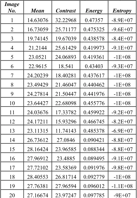
Feature vectors are extracted from skull stripped image and these features are given as input to SVM classifier. The features obtained for training set are shown in Table1 and Table2.
Table 1: Features for Normal Images in the Training Set
Image
No. Mean Contrast Energy Entropy
1 14.63076 32.22968 0.47357 -8.9E+07 2 16.73059 25.71177 0.475325 -9.6E+07 3 19.74145 19.67039 0.438578 -8.4E+07 4 21.2144 25.61429 0.419973 -9.1E+07 5 23.0521 24.06893 0.419361 -1E+08 6 22.9615 18.541 0.43403 -9.3E+07 7 24.20239 18.40281 0.437617 -1E+08 8 23.49429 21.46047 0.440462 -1E+08 9 24.27814 21.50447 0.441976 -1E+08 10 23.64427 22.68098 0.455776 -1E+08 11 24.03676 17.33782 0.459922 -9.2E+07 12 24.17211 15.93296 0.466745 -8.2E+07 13 23.11315 11.74143 0.485378 -6.9E+07 14 26.73612 27.0846 0.090421 -8.8E+07 15 28.16424 23.96585 0.088344 -8.8E+07 16 27.96912 23.4885 0.089495 -9.1E+07 17 27.72102 23.58369 0.091976 -9.8E+07 18 28.40553 26.81714 0.092779 -1E+08 19 27.76381 27.96594 0.096012 -1.1E+08 20 27.16674 23.97247 0.097785 -9E+07
Image
No. Correlation Homogeneity Variance
1 0.992259 0.856485 48.05882 2 0.993404 0.863112 50.4175 3 0.995164 0.858315 53.86453 4 0.994063 0.855283 57.51562 5 0.99488 0.850947 63.42453 6 0.994728 0.861084 66.78054 7 0.994564 0.866539 68.10991 8 0.993828 0.868176 68.34244 9 0.993779 0.867323 67.63884 10 0.994274 0.864738 66.17371 11 0.995499 0.860605 65 12 0.996475 0.85509 63.40208 13 0.996856 0.860246 61.71113 14 0.994206 0.809452 57.25596 15 0.994858 0.803385 63.39588 16 0.994164 0.805304 65.52551 17 0.993835 0.815988 66.83987 18 0.993407 0.815467 67.22114 19 0.992838 0.819602 66.79257 20 0.995518 0.811588 63.84878
Table 2: Features for Abnormal Images in the Training Set
Image
No. Mean Contrast Energy Entropy
ISSN 2348 – 7968
638 18 17.75243 22.59145 0.457628 -1.2E+08
19 40.99082 22.02775 0.056417 -1.1E+08 20 25.37896 8.180371 0.109712 -8.9E+07
Image
No. Correlation Homogeneity Variance
1 0.993027 0.820649 72.07118 2 0.984374 0.782691 47.84119 3 0.987778 0.782571 48.73723 4 0.991619 0.856358 69.64702
5 0.992254 0.82793 61.65136
6 0.988411 0.791417 73.80054 7 0.991806 0.802904 62.3205 8 0.993751 0.861614 58.99735 9 0.989713 0.791531 75.9695 10 0.985245 0.794729 105.9683 11 0.989694 0.822959 50.08406 12 0.988117 0.814459 66.81027 13 0.989598 0.802265 73.3194 14 0.995972 0.79245 70.57637 15 0.995755 0.815019 58.50058 16 0.99467 0.847287 71.48729
17 0.9934 0.808423 77.18869
18 0.991987 0.861208 57.00186 19 0.996821 0.780674 95.30825 20 0.990849 0.853068 65.90526
SVM classifier is used with linear kernel function and accurate classification results are obtained for all the test images for different abnormal cases and normal cases with an execution time of 6.128833 seconds.
7. Conclusions
The proposed method for classification of abnormalities in brain MRI images using SVM classifier gives better results compared to other techniques. Skull stripping algorithm removes the skull region which is not necessary for abnormality detection thereby reducing the execution time and increasing efficiency. This system can further be used to detect specific abnormality present in the image by modifying the SVM classifier into Multiclass SVM classifier.
References
[1] Rajeswari.S, and Theiva Jeyaselvi.K, "Support Vector Machine Classification for MRI Images", International Journal of Electronics and Computer Science Engineering, Vol. 1, No. 3, 1956, pp.1534-1539.
[2] D.Singh, and K.Kaur, "Classification of Abnormalities in Brain MRI Images Using GLCM, PCA and SVM", International Journal of Engineering and Advanced Technology, Vol. 1, No. 6, 2012, pp.243-248.
[3] Sonali Patil and Dr.V.R.Udupi, "Preprocessing to be Considered for MR and CT Images Containing Tumors", IOSR Journal of Electrical and Electronics Engineering, Vol. 1, No. 4, 2012, pp.54-57.
[4] P.Mohanaiah, P.Satyanarayana and L.GuruKumar "Image Texture Feature Extraction Using GLCM Approach", International Journal of Scientific and Research Publication, Vol. 3, No. 5, 2013, pp.1-5.
[5] Fritz Albregtsen, "Statistical Texture Measures Computed From Gray Level Co Occurrence Matrices", Image Processing Laboratory, Department of Informatics, University of Oslo , 2008, pp.1-14.
[6] R .Harclick, K. Shanmugam, I. Dinstein, “Texture Features
For Image Classification”, IEEE Transaction, vol3, No 6,
1973, pp.610-621.
[7] N. Otsu, “A Threshold Selection Method from Gray- Level
Histogram”, IEEE Trans.on System Man Cybernetics, vol.9
1979, 9962-66.
[8] M.M.Mokji and S.A.R. Abu Bakar, "Gray Level Co Occurrence Matrix Computation Based on Haar Wavelet", Computer Graphics, Imaging and Visualization, 2007. [9] Rosy Kumari, "SVM Classification An Approach on
Detecting Abnormality in Brain MRI Images", International Journal of Engineering Research and Applications, Vol. 3, No. 4, 2013, pp.1686-1690.
Namratha D’cruz has completed her Bachelor of Engineering in
Electronics and communication from Vidyavardhaka College of Engineering, Mysuru, Karnataka, India in the year 2013. Presently she is pursuing M.Tech in Signal Processing in Vidyavardhaka College of Engineering, Mysuru, Karnataka, India. Her areas of interest include Medical Image Processing and Speech Processing.
Sudheesh K.V has completed his Bachelor of Engineering in Electronics