Scholarship@Western
Scholarship@Western
Electronic Thesis and Dissertation Repository
4-12-2013 12:00 AM
Rigid Body Attitude Estimation: An Overview and Comparative
Rigid Body Attitude Estimation: An Overview and Comparative
Study
Study
Nojan Madinehi
The University of Western Ontario Supervisor
Dr. Abdelhamid Tayebi
The University of Western Ontario
Graduate Program in Electrical and Computer Engineering
A thesis submitted in partial fulfillment of the requirements for the degree in Master of Engineering Science
© Nojan Madinehi 2013
Follow this and additional works at: https://ir.lib.uwo.ca/etd Part of the Controls and Control Theory Commons
Recommended Citation Recommended Citation
Madinehi, Nojan, "Rigid Body Attitude Estimation: An Overview and Comparative Study" (2013). Electronic Thesis and Dissertation Repository. 1259.
https://ir.lib.uwo.ca/etd/1259
This Dissertation/Thesis is brought to you for free and open access by Scholarship@Western. It has been accepted for inclusion in Electronic Thesis and Dissertation Repository by an authorized administrator of
(Thesis format: Monograph)
by
Nojan Madinehi
Graduate Program in Electrical and Computer Engineering
A thesis submitted in partial fulfillment
of the requirements for the degree of
Master of Engineering Science
The School of Graduate and Postdoctoral Studies
The Western University
London, Ontario, Canada
c
The attitude estimation of rigid body systems has attracted the attention of many re-searchers over the years. The development of efficient estimation algorithms that can ac-curately estimate the orientation of a rigid body is a crucial step towards a reliable imple-mentation of control schemes for underwater and flying vehicles.
The primary focus of this thesis consists in investigating various attitude estimation techniques and their applications.
Two major classes are discussed. The first class consists of the earliest static attitude determination techniques relying solely on a set of body vector measurements of known vectors in the inertial frame. The second class consists of dynamic attitude estimation and filtering techniques, relying on body vector measurements as well other measurements, and using the dynamical equations of the system under consideration.
Various attitude estimation algorithms, including the latest nonlinear attitude observers, are presented and discussed, providing a survey that covers the evolution and structural differences of these estimation methods.
Simulation results have been carried out for a selected number of such attitude estima-tors. Their performance in the presence of noisy measurements, as well as their advantages and disadvantages are discussed.
Keywords:Rigid Body, Attitude Estimation, Inertial Measurement Units, Kalman Fil-tering, Observer Design
First and foremost, I would like to offer my utmost gratitude to my supervisor Dr. Ab-delhamid Tayebi, Professor, Department of Electrical Engineering, Lakehead University, whose gracious support, ever-present guidance, encouragement and invaluable assistance paved my way to culminate this dissertation. I am highly thankful to Dr. Tayebi for pro-viding me the opportunity to work in this area of research.
I acknowledge the support of my co-supervisor Dr. Ilia G. Polushin, Assistant Profes-sor, Department of Electrical and Computer Engineering, Western University, whose help and guidance has always been to the highest degree. I am grateful to Dr. Rajni Patel, Distin-guished University Professor and Tier-1 Canada Research Chair, Department of Electrical and Computer Engineering, Western University and Dr. Vijay Parsa, Department of Elec-trical and Computer Engineering, Western University, for building my foundations in the fields of optimization and filtering.
I would also like to offer my sincere appreciation to Dr. Bjarni Tryggvason, Distin-guished Astronaut and University Professor, for his hands-on experience with the sensor measurements, something that helped me to better understand the real world.
Special thanks to Faraz Shah, Amir Takhmar, Zayed Hasan and Farshad Anoushahpour for their great support as colleagues and providing me a wonderful working experience.
Last but not the least, I would like to thank my parents Giti and Isa. They were always supportive and encouraging throughout the time. Also to Nazli, for her enthusiasm, interest and support throughout this project.
Abstract ii
Acknowledgement iii
List of Figures vi
1 General Introduction 1
2 Attitude Representation and Mathematical Preliminaries 5
2.1 Introduction . . . 5
2.1.1 Coordinate Frames . . . 6
2.2 Attitude Parameterizations . . . 6
2.2.1 Direction Cosine Matrix . . . 6
2.2.2 Euler Angles . . . 8
2.2.3 Unit Quaternion . . . 9
2.3 Rigid Body Kinematics and Dynamics . . . 12
2.3.1 SO(3) and SE(3) . . . 13
2.4 Sensor Measurements . . . 15
2.4.1 Rate Gyros . . . 16
2.4.2 Magnetometers . . . 16
2.4.3 Accelerometers . . . 17
3 Static Attitude Determination 18 3.1 Introduction . . . 18
3.2 TRIAD . . . 20
3.3 SVD and FOAM . . . 20
3.4 Q-Method and the QUEST . . . 22
3.5 Recursive QUEST Algorithms . . . 26
3.6 Extended QUEST . . . 28
3.7 Sequential Optimal Attitude Recursion Filter . . . 30
3.8 Simulations . . . 33
3.8.1 Parameters and Conditions . . . 33
3.8.2 Error Definitions . . . 34
3.8.3 QUEST . . . 35
4 Dynamic Attitude Filtering and Estimation 39
4.1 Introduction . . . 39
4.2 Extended Kalman Filters . . . 41
The Basics of Extended Kalman Filtering . . . 42
Multiplicative EKF . . . 44
Additive EKF . . . 46
4.2.1 Unscented Kalman Filters . . . 48
4.2.2 Invariant Kalman Filters . . . 52
4.3 Linear Complementary Filters . . . 54
4.4 Symmetry-Preserving and Invariant Observers . . . 60
4.4.1 Gradient Observers . . . 63
4.5 Nonlinear Complementary Filters . . . 69
4.5.1 Explicit Complementary Filter and Compatible Observers . . . 74
4.6 Global Attitude Estimators Evolving Outside SO(3) . . . 81
4.7 Velocity-Aided Attitude Estimation . . . 88
4.8 Nonlinear Observers on SE(3) . . . 93
4.9 Simulations . . . 104
4.9.1 Invariant EKF . . . 105
4.9.2 Unscented EKF . . . 106
4.9.3 Nonlinear Complementary Filter . . . 108
4.9.4 Velocity-aided Attitude Observer . . . 110
4.9.5 Global Observer non-evolving on SO(3) . . . 112
4.9.6 Invariant Observer . . . 116
4.10 Discussion . . . 117
5 General Conclusion 124
Bibliography 127
Curriculum Vitae 142
2.1 The fixed Inertial frame with the moving body frame . . . 14 3.1 Error Euler angles of the QUEST algorithm with ideal noise-free IMU
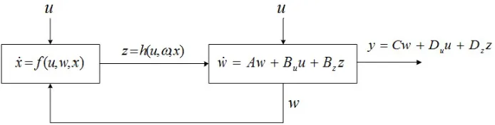
sen-sor measurements. . . 36 3.2 Error Euler angles of the QUEST algorithm with noisy measurements. . . . 37 3.3 Error Euler angles of the Filter QUEST algorithm with noisy measurements. 37 4.1 Block diagram of the interconnected nonlinear and linear systems, from
[Grip et al., 2012b] . . . 83 4.2 Block diagram of the rotational and transitional dynamics of a flying
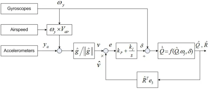
vehi-cle expressed in a cascaded structure. . . 83 4.3 Block diagram of the complementary filter with airspeed measurements,
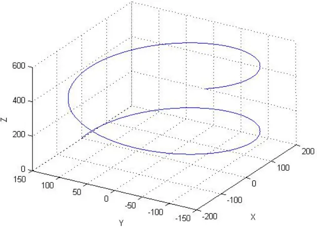
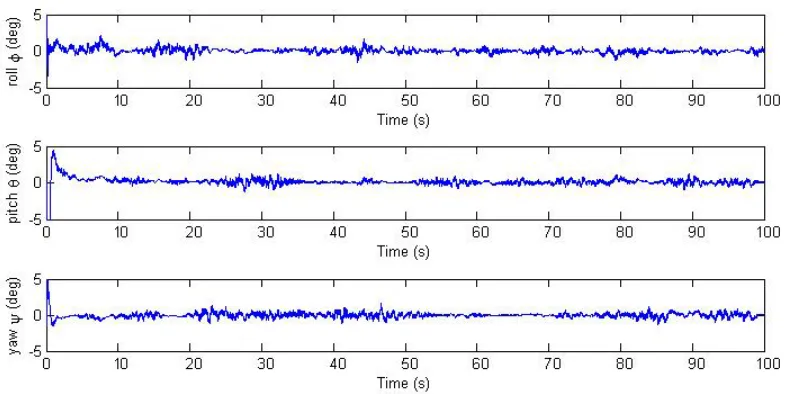
from [Mahony et al., 2011] . . . 93 4.4 The trajectory of the rigid body position in a 100 seconds time interval. . . . 104 4.5 Error Euler angles of the Invariant Extended Kalman Filter under the
as-sumption of noisy IMU measurements and accelerated motion. . . 106 4.6 Error Euler angles obtained from the Unscented Kalman Filter under noisy
measurements condition. . . 107 4.7 Error Euler angles of the nonlinear complementary filter with ideal
noise-free sensor measurements. . . 108 4.8 Error Euler angles of the nonlinear complementary filter under noisy
mea-surements condition. . . 109 4.9 The effect of the linear acceleration of the rigid body on the error Euler
angles of the nonlinear complementary filter with noise-free measurements. 110 4.10 Error Euler angles of the nonlinear complementary filter in accelerated
mode with noisy measurements. . . 111 4.11 Performance of the velocity-aided algorithm under noise-free measurements
assumption (Accelerated mode) . . . 112 4.12 Performance of the velocity-aided algorithm with noisy measurements
(Ac-celerated mode) . . . 113 4.13 (a) Convergence of the auxiliary matrixA toR ∈ SO(3), (b) Convergence
of the attitude error norm to zero. . . 114 4.14 Performance of the velocity-aided observer with auxiliary matrix not
be-longing toSO(3) in noisy measurements condition. . . 115
4.16 Performance of the global observer non-evolving onS O(3) with noisy mea-surements (Accelerated mode) . . . 117 4.17 Error Euler angles of the invariant observer with ideal measurements
(Ac-celerated mode) . . . 118 4.18 Error Euler angles of the invariant observer with noisy measurements
(Ac-celerated mode) . . . 119
General Introduction
The aerial robotics field has seen a growing interest during the last few decades because of its remarkable achievements in providing flying vehicles that can assist humans in a variety of difficult and hazardous tasks. Some examples of where these robotic systems may be employed include outer space (such as Earth-orbiting satellites), surveying and inspecting structures (such as tall skyscrapers and huge dams), investigation of hazardous or toxic environments, and traffic congestion and security applications. Such operations require aerial vehicles with a certain level of autonomy and manoeuvrability.
Unmanned Aerial Vehicles (UAVs) have shown great potentials in many indoor and outdoor applications. These vehicles can either be very large or relatively small in size depending on the applications they are intended to. From the heavy weight military drones to small vertical take-offand landing (VTOL) UAVs, the control of all these flying vehicles relies on some crucial sensors that provide the necessary flight information.
The UAV position, orientation and velocities are crucial states that need to be measured or estimated for the implementation of a successful motion control strategy. The position and linear velocity can be obtained using a Global Positioning System (GPS) for instance, while the angular velocity can be obtained using a body-attached gyroscope. As for the orientation (attitude), there is no sensor that measures it directly. However, the orientation is usually obtained using some attitude estimation algorithms relying on gyroscopic and
body vector measurements.
The earliest attempts to estimate the attitude of flying vehicles may go back to the time when mechanical gyroscopes, which provide measurements of angular velocity, were used in an integration process in which the knowledge of an initial attitude would be sufficient in finding the attitude in any other time. However, since these devices were primitive and usually had many problems with pressure, heat, etc., their ultimate performance was not satisfying and frequent restarting of the estimation process was required. With the advances in electronic devices, microelectromechanical systems (MEMS) have replaced those previous measurement devices. These components have provided low cost and light weight Inertial Measurement Units (IMUs) for both industrial and research applications. The use of body vector measurements sensors such as accelerometers and magnetometers have allowed researchers to design better attitude estimation algorithms.
Probably one of the first and yet most influential works in the attitude estimation field was a mathematical problem proposed by Wahba in [Wahba, 1965]. The problem con-sists in finding the optimal attitude rotation matrix provided that a number of vectorial measurements are available. Several attempts to solve this problem resulted in the devel-opment of fast estimation methods, such as the Singular Value Decomposition (SVD) in [Markley, 1988], Quaternion Estimation (QUEST) in [Shuster and Oh, 1981], and Filter QUEST in [Shuster, 1989b], which were used in some of the NASA projects in 1980’s. Various solutions to the Wahba’s problem are categorized as a class of attitude estimators known as deterministic attitude estimators.
estimation problems, such as the IBM Space Precision Attitude Reference System (SPARS) ([Toda et al., 1969b]).
Despite the popularity of conventional EKFs, their dependence on the linearization of system equations was a disadvantage that could result in filter divergence. Therefore, some researchers tried to propose alternative estimation methods that did not require the linearization process. The Unscented Kalman Filtering (UKF) technique developed in [Julier and Uhlmann, 2004] relies on a set of points known as sigma points to estimate the mean of states and their covariance matrix. The method was specifically applied to atti-tude estimation applications in [Crassidis and Markley, 2003] and [VanDyke et al., 2004]. Another approach which consists in estimating the Probability Density Function (PDF) of states, known as Particle Filtering (PF), has been investigated in [Cheng and Crassidis, 2004], [Liu et al., 2007] and [Carmi and Oshman, 2009b] for attitude estimation purposes.
In the last decade, the emergence of a new and powerful class of attitude estimation techniques, relying on nonlinear observers, has brought new hopes for more reliable and stable attitude estimators. Rigorous stability proofs and strong mathematical arguments for the performance of nonlinear attitude observers are regarded as their important advantages over conventional filtering techniques.
Attitude filters with nonlinear structures such as the ones proposed in [Salcudean, 1991], and [Thienel and Sanner, 2003] inspired a number of subsequent works that led to a variety of nonlinear attitude filters and observers (e.g.,[Mahony et al., 2008], [Tayebi et al., 2011]). These observers can estimate not only the attitude, but other system states and unknown parameters and have been shown to have good performance under noisy measurement conditions. Various solutions to the problems associated with real-time applications of these observers, in accelerated flights for instance, have been developed in [Hua, 2010], [Roberts and Tayebi, 2011b], and [Grip et al., 2012b].
provided researchers with remarkable achievements in the attitude estimation field.
Other types of nonlinear attitude observers include those that provide simultaneous es-timates of the rotational and translational states and are best suited for navigation purposes. The algorithms presented in [Rehbinder and Ghosh, 2003] and [Baldwin et al., 2007] rely on vision systems, and are shown to be efficient in indoor applications.
One of the objectives of this thesis is to provide a survey of the latest developments in the field of attitude estimation with an emphasis on the nonlinear observer techniques. Although there have been a number of attitude estimations surveys, such as
[Lefferts et al., 1982] and [Crassidis et al., 2007], to the extent of the author’s knowledge, there has been no surveys on the newly developed nonlinear attitude observers. The impor-tance of this work is that a thorough study of this class of attitude estimation techniques may pave the way for other researchers to not only get familiar with nonlinear attitude ob-servers, but develop new tools with better performance. Nonlinear observers have great potentials for further research and this survey tries to enlighten this by providing informa-tion on the evoluinforma-tion and achievements of these tools.
Attitude Representation and
Mathematical Preliminaries
2.1
Introduction
In aerospace engineering, it is often needed to know the orientation of rigid bodies in space with respect to a reference frame attached to the Earth, the Sun, or the stars. The aim of this chapter is to review some of the commonly used attitude parameterizations used to describe a spacecraft’s orientation. The properties of these attitude parameterizations are discussed with their relative advantages and disadvantages in section (2.2). For a more complete and comprehensive discussion on different ways of representing the attitude, readers are referred to [Stuelpnagel, 1964a], [Shuster, 1993], and [Hughes, 1986].
The dynamic equations of motion for a rigid body with a brief introduction to the kine-matic equations are presented in section (2.3). Their introduction helps define the special groups that represent the rotational and translational motion. Section (2.3.1) is dedicated to this aim.
Since the application of sensor measurements in attitude estimation problems is numer-ously discussed through this survey, section (2.4) will be including a brief introduction to the sensors pertinent to the attitude estimation problem.
2.1.1
Coordinate Frames
Let I denote an inertial (fixed) frame and let B denote the body-attached frame. The orientation (attitude) of a rigid body is defined as the orientation of frameBwith respect to frameI.
The attitude of a rigid body can be expressed by a variety of mathematical parameter-izations, which can be either constrained with redundant elements, or unconstrained with minimal elements. The rotation matrix and the unit-quaternion are examples of constrained parameterizations and Euler angles, the Rodrigues parameters and the modified Rodrigues parameters (MRPs) are examples of minimal parameterizations.
In this section, we briefly review the most common attitude representations which are the rotation matrix, unit-quaternion and Euler angles. These parameterizations constitute the bases of most attitude estimation techniques and their properties and group structures are of great importance for the study of the evolution of attitude filters and observers.
2.2
Attitude Parameterizations
2.2.1
Direction Cosine Matrix
The Direction Cosine Matrix (DCM), commonly known asrotation matrix, is a widely used attitude representation and an element of the Lie groupSO(3), that is the special orthogonal group of dimension 3,
SO(3) :={R∈R3×3|RTR= RRT = I3×3,det(R)=1}. (2.1)
This definition points to the orthogonal basis of columns in a rotation matrix, making it an orthogonal matrix itself. In this case, the inverse of matrix is equal to its transpose, i.e. RT =R−1.
There are two definitions of rotation matrix: one that relates the orientation from the body-fixed frame Bto the inertial reference frameI, and the other that carriesIinto the
representation is used, both definitions represent the same concept and can be easily trans-formed into each other. LetR ∈SO(3) be the rotation matrix describing the orientation of a rigid body, and letω:= (ω1, ω2, ω3)T be the angular velocity of the rigid body expressed
in the body frame. Then, the rigid body kinematics equation is given by
˙
R= RS(ω), (2.2)
whereS(x) denotes the skew-symmetric matrix associated tox. The skew symmetric ma-trixS(x) satisfiesS(x)y= x×y, ∀x,y ∈R3, where (× ) denotes the vector cross product, and is given by
S(ω)=
0 −ω3 ω2
ω3 0 −ω1
−ω2 ω1 0
. (2.3)
For a rotation matrix from the inertial frame to the body frame, the kinematics equation equivalent to (2.2) is expressed as
˙
R= −S(ω)R. (2.4)
The rotation matrix is a global and unique representation of orientation. Using this matrix, related vectors in reference coordinates of inertial and body frames can be mapped to each other. For example, letaI be a vector expressed in the inertial frameIandaBbe the vector coordinates ofaIexpresses in the body frameB. Then,
aB =RTaI. (2.5)
2.2.2
Euler Angles
Euler angles are Euclidean parameterizations that lie inR3. Among all the different
dimensional parameterizations, Euler angles are the most widely used. A number of three-dimensional attitude parameterizations are presented and discussed in [Stuelpnagel, 1964b]. It is shown that no such parameterization can be both nonsingular and unique, which is also the case for Euler angles. The components of the vector of Euler anglesΘ = [φ, θ, ψ]T, are referred to as theroll,pitchandyawof the rigid body.
Given two coordinate systems xyzand x000y000z000, the process by which the three Euler angles transform the first coordinate system into the second system can be summarized as follows:
1. A positive rotation by an angleψabout thezaxis, leading to x0y0z0 wherez≡z0. 2. A positive rotation by an angleθabout the x0axis, leading to x00y00z00wherex00 ≡ x0. 3. A positive rotation by an angleφabout they00 axis, leading tox000y000z000 wherey000 ≡
y00.
The rotation matrix can be obtained as a product of three different rotation matrices, each corresponding to a rotation about three axes of the body frameB. This is given by
R=
cψ −sψ 0
sψ cψ 0
0 0 1
cθ 0 sθ
0 1 0
−sθ 0 cθ
1 0 0
0 cφ −sφ
0 sφ cφ
, =
cθcψ sθsφcψ− sψcφ sθcφcψ+sψsφ cθsψ sθsφsψ+cψcφ sθcφsψ−cψsψ
−sθ cθsφ cθcφ
, (2.6)
deriva-tive of the Euler angles in light of (2.2) reads
˙
φ=ω1+ sφtanθ ω2+cφtanθω3,
˙
θ=cφω2− sφω3,
˙
ψ= sφ(cθ)−1ω2+cφ(cθ)−1ω3.
(2.7)
The Euler angles parameterization is not global and anglesφandψalong with their deriva-tives are not well-defined for θ = ±π/2. This problem is not unique for the Euler angles
parameterization and all other three-dimensional parameterizations have a similar singular-ity problem.
2.2.3
Unit Quaternion
Unit quaternion is a four-dimensional parameterization of attitude that allows avoiding singularities associated with the three-dimensional parameterizations. Euler was the first scientist to discover the abilities of this formulation and found out that an axis can be assigned to every rotation in three-dimensional space. This can be stated as follows:
Euler’s Theorem: Consider an element R of the Special Orthogonal group. For any rotation matrixR∈SO(3), a non-zero vector xexists that satisfiesRx= x.
The existence of vector x that remains unchanged under a transformation of rotation matrix multiplication implies that any attitude can be specified in terms of a rotation by some angle about some fixed axis. Therefore, combination of a vector with a scalar can make a basis for attitude parameterization. The equality Rx = λx also indicates that any rotation matrix has an eigenvalue equal to one. A new proof to the Euler’s theorem is recently presented in [Palais and Palais, 2007].
com-munity.
The unit quaternion is denoted byQ = (q0,q) ∈Q, whereq0 ∈ Ris its scalar part and q= (q1,q2,q3)∈R3its vector part. The non-Euclidean set of unit quaternions is defined by Q:= {Q∈R×R3| |Q|2= 1}. (2.8)
As a result of the norm constraint in their definition, it can be seen that unit quaternion forms a unit sphere in R4. As previously discussed, it is known from the Euler’s theorem
that the attitude of a rigid body can be described in terms of a rotation by some angle θ along an axis ˆk. This gives another definition of quaternion
Q=(q0,q)= (cos(θ/2),sin(θ/2)ˆk), (2.9)
whereθis the angle of rotation and ˆkis a unit length rotation axis.
There is a simple transformation of a unit quaternion into its corresponding rotation matrix which is known as theRodrigues formulaand is given by
R(Q)= I3+2S(q)2−2q0S(q), =
q2
0+q21−q22−q23 −2q0q3+2q1q2 2q0q2+2q1q3
2q0q3+2q1q2 q20−q21+q22−q23 −2q0q1+2q2q3
−2q0q2+2q1q3 2q0q1+2q2q3 q20−q12−q22+q23
. (2.10)
Apart from quaternion, rotation matrix can also be constructed using the rotation angle θ and rotation axis ˆkby the following transformation
R(θ,kˆ)= I3−sin(θ)S(ˆk)+(1−cos(θ))S(ˆk)2. (2.11)
While the rotation spaceSO(3) has three-elements, quaternion representation has four elements which make it an over-parameterization of this space. This results in the transfor-mation fromQ→SO(3) to form a two-to-one map. In fact, it is obvious from ( 2.10 ) that
orientation in space. Despite, this redundancy, the unit-quaternion representation is a non-singular (global) representation of the attitude.
Given two unit quaternionsQx = (q0,x,qx) and Qy = (q0,y,qy), the quaternion product denoted byQz =(q0,z,qz) is defined as
Qz= Qx⊗Qy =
q0,xq0,y−qTxqy q0,xqy+q0,yqx+qx×qy
, (2.12)
where (⊗) denotes the quaternion multiplication and (×) denotes the cross product. It should be noted that the quaternion multiplication is not commutative and Q1 ⊗ Q2 , Q2⊗Q1. The inverse of a quaternion denoted byQ−1is defined asQ−1= (q0,−q), where
Q⊗Q−1 = Q−1⊗Q=(1,0). (2.13) The kinematics of unit quaternion attitude representation is given by the following equa-tion
˙
Q= 1
2Q⊗(0, ω)= 1 2
−qT q0I+S(q)
ω. (2.14)
The unit quaternion has some advantages over the other attitude parameterizations. One advantage is that it works with a 4× 1 vector rather than a 3 × 3 (9 elements) attitude matrix. This not only makes work and computations easy, it also helps in applications where normalization of attitude representation is needed because of perturbations involved in its estimation process; normalizing a unit quaternion by simply dividing by its norm is much easier than the non-trivial process of preserving the orthogonality of a rotation matrix.
2.3
Rigid Body Kinematics and Dynamics
The dynamic model of a rigid body or a flying vehicle consists of its rotational and transla-tional motion. Based on the chosen attitude parameterization method, the rotatransla-tional kine-matics equation takes different forms which were presented for rotation matrix (2.2), Euler angles (2.7), and unit quaternions (2.14). Recallingω ∈ R3as the body-measured angular velocity expressed in B, the complete rotational dynamic equations of a flying rigid body using the rotation matrix representation is given by
˙
R= RS(ω), Ibω˙ = −ω×Ibω+u,
(2.15)
where Ib ∈ R3×3 denotes the inertia matrix of rigid body, andu ∈ R3 is the control torque
input applied to the rigid body. In practice, the torque is computed according to the desired control strategy and is a function of estimated system parameters and states.
Let us denote the position and linear velocity of the rigid body with respect to the earth-fixed frame, by pandvrespectively. The simplified translational dynamics of a flying rigid body can be expressed as follows
˙
p=v,
˙
v=ge3+RTa,
(2.16)
wheree3= [0,0,1]T is the body-referenced z-axis andais thespecific accelerationvector
that is the sum of all the non-gravitational forces divided by the body massm. gis the Earth gravitational acceleration given by g ≈ 9.8m/s2. Note that these equations are ideal and
external forces and torques were not included. In practice, these forces play an important role in the process of designing controllers for aerial vehicles, such as small aircrafts. More complex system models that take the disturbance forces and torques into account are found in the works of [Roberts and Tayebi, 2011a] and [Pflimlin et al., 2007].
and an IMU are available. These estimators provide estimates of not only the attitude of a flying vehicle, but its position and velocity.
2.3.1
SO(3) and SE(3)
In the study of rotational and translational dynamics of flying objects, it is always useful to refer to some special groups on which these dynamics are defined. The two groups are known as Special Orthogonal group SO(3) and Special Euclidean group SE(3). Be-cause of the importance of the properties of these groups when dealing with nonlinear observers of special structures, a brief explanation of their properties is presented in this section. Detailed information on the structure of these two special groups can be found in [Belta and Kumar, 2002].
LetGL(n) be the general linear group of dimension n. This group is a subset ofRn×n
and by definition, matrix operations of multiplication and inversion are smooth. Therefore,
GL(n) is a Lie group. The Special Orthogonal groupSO(n) is defined as a subgroup of this general linear group given by
SO(n)={R|R∈GL(n),RRT = RTR= In×n,detR=1}. (2.17) TheSO(n) describes the rotation group onRn. The affine groupGA(n) is defined asGA(n)=
GL(n)×Rn, and the set of all rigid displacements in
RnisS E(n)= SO(n)×Rn. In the special
case of three-dimensional space R3, SO(3) and SE(3) refer to the rotation group, and the
group that includes both translations and rotations, respectively.
Figure 2.1: The fixed Inertial frame with the moving body frame .
in three dimensions
SE(3)={T ∈R4×4|T =
R p
0 1
,R∈SO(3),p∈R3}. (2.18) This representation of an element of SE(3) is commonly known as homogeneous coor-dinates. The group is a closed subset of GA(3) and a Lie group. The inverse element associated withT is
T−1 =
RT −RTp
0 1
=
RT P
0 1
, (2.19)
whereP = −RTpis the position of the vehicle in the body frame. LettingV = RTvdenote the translational velocity of the vehicle inB, the standard expressions for the kinematics in inertial frame and body frame are given by
˙
p=v,
˙
P=S(ω)P−V.
(2.20)
Using the kinematics equations of rigid body, the kinematics of SE(3) element T are given by
˙
where the matrixA∈R4×4denotes the body-fixed frame velocity of the system A=
S(ω) V
0 0
. (2.22)
2.4
Sensor Measurements
Most of the available estimators of attitude and pose, such as the nonlinear observers and Kalman filters, use the knowledge of system inputs and measured outputs to predict the system states. Once the system states are predicted, the estimated outputs are obtained and compared to the existing outputs of the real system to correct the next prediction. For a dynamical system in a form of a rigid-body in space, the inputs are the applied torques and forces and the outputs are attitude and position of the system.
The most common and widely available sensor package that is used for estimation in aerial vehicles, specially the small-scale UAVs, are Inertial Measurement Units (IMUs), which provide the measurements of angular velocity, the magnetic field intensity in the surrounding environment, and the linear acceleration of the rigid body. These units are generally very cheap and small, with a total weight less than 50 grams. Although the read-ings of these sensors are prone to measurement noise, their availability and small size have made them perfect choices for estimation and control purposes in Aerial and Aeronautics applications. For a comprehensive study on the available IMU sensors, readers are referred to [Chao et al., 2010].
interest for industrial purposes. As evident from most scientific publications, the applica-tion of IMUs are far more common than visual tracking sensors. Therefore, this survey provides only a brief description of performance of the common IMUs used in attitude observers and filters design.
2.4.1
Rate Gyros
The Gyroscopes or Rate Gyros provide measurements of the angular velocity of the body-fixed frame Brelative to the inertial frame I, expressed inB. Letω ∈R3 be the system’s actual angular velocity, andωy ∈R3 be the measured output given by
ωy = ω+ωb+nω, (2.23)
wherenω denotes the measurement noise andωb denotes the existing bias in readings. In practice, the gyro bias is constant or slowly time-varying. Therefore, in many applications the dynamics of this bias is taken as
˙
ωb≈ 0. (2.24)
2.4.2
Magnetometers
The magnetometers measure the magnetic field in the surrounding environment. letmI ∈
R3 be the constant, known magnetic field in an area and let mB ∈ R3 denote the body-expressed vector associated with mI. The magnetometer reading my, expressed in B, is then given by
my = mB+nm,
= RTmI+nm,
(2.25)
wherenmdenotes the magnetometer’s measurement noise.
vehicle with electric motors. Although most research works have not considered the varia-tions of magnetic field in a typical short-distance flight, the work in [Vissiere et al., 2007] have investigated the magnetic field changes according to Maxwell’s laws in environments where GPS data is not available and proposed a Kalman-based attitude estimation tech-nique.
2.4.3
Accelerometers
These sensors measure the instantaneous linear acceleration of the body frame with respect to the inertial frame minus the gravitational acceleration field. Let the vehicle’s linear acceleration, expressed inIbe denoted as ˙v, and letg = ge3 be the vector of gravity that
points to centre of Earth in a NED coordinate. Then the output of a set of accelerometers, denoted asa, is
a= RT(˙v−g)+na, (2.26) with na representing the measurement noise. In many cases where the rigid body is not having an accelerated motion, the norm of gravity field vector (|g| ≈ 9.8) dominates other
terms and can be assumed to be the only measured value. In this case, the following ap-proximation holds
a≈ −RTg. (2.27)
This is an estimate of the z axis in I, that is measured and expressed in B. It will be shown in section (4.5) that such low-frequency estimate of a fixed vector in local frame is a fundamental requirement in the design of some filters and observers, notably nonlinear complementary filters.
Static Attitude Determination
3.1
Introduction
Static Attitude Determination is probably the oldest systematic trend of estimating the at-titude of a flying vehicle with acceptable accuracy. This class of atat-titude estimation tech-niques takes advantage of the body vector observations to numerically determine the at-titude without necessarily considering its kinematics. In this way, the atat-titude is merely regarded as a matrix (or quaternion) that transforms a vectorx ∈R3 in one frame to a
vec-tory ∈R3 in another frame and as a result, can be obtained by mathematical optimization
techniques. Therefore, the information of the original system’s dynamics is disregarded and attitude is found on an optimization basis.
The method, also known asdeterministic solution, is characterized by finding the at-titude estimate in a single point in time when observations of some known vectors in the inertial frame are available in the body frame. It has a simple estimation process with rela-tively small computational cost. However, this comes with a lower accuracy than the other methods that rely on additional information of the system dynamics.
Although the earliest deterministic solution techniques relied only on body vector mea-surements and literally put the system equations aside, the emergence of recursive tech-niques that considered system dynamics for propagation of states in late 1990s provided
more reliable methods with remarkable resemblance to the Kalman filters.
Major development of these methods, also known asbatch attitude determination algo-rithms, started with the early optimization methods proposed to solve the Wahba’s problem [Wahba, 1965]. In this problem, with the assumption that two sets of simultaneously ob-served unit vectors ˆV1, ...,VˆN and ˆW1, ...,WˆN are respectively known in the inertial frame (i.e. the reference coordinate system) and the body frame, orthogonal matrixR, represent-ing the rotation matrix, is numerically found by minimizrepresent-ing the loss function
L(R)= 1 2
N X
i=1
ai|Wˆi −RVˆi|2, (3.1) where theai,i = 1, ...,N are non-negative weights andN is the number of measurements. By normalizing these weights to havePN
i=1ai =1, it is straightforward to show that
L(R)= 1−
N X
i=1
aiWˆiTRVˆi =1−tr(RBT), (3.2) where tr denotes the trace operator and matrix Bis defined as
B= N X
i=1
aiWˆiVˆiT. (3.3)
Equation (3.2) reduces the problem to finding the appropriate matrixRthat maximizes the term tr(RBT). It should be noted that Wahba’s problem addresses the attitude determi-nation in a closed-form reconstruction manner. For generalizations of this problem readers are referred to [Shuster, 2006] and [Psiaki, 2010].
3.2
TRIAD
The earliest attitude reconstruction method, known as TRIAD [Lerner, 1978], was designed to work with only two non-collinear unit reference vectors ˆV1,Vˆ2in inertial frame and their
corresponding unit observation vectors ˆW1,Wˆ2in body frame to construct new orthonormal
reference with bases (ˆr1,rˆ2,rˆ3) and observation vectors (ˆb1,bˆ2,bˆ3):
ˆ
r1 =Vˆ1,rˆ2 = ( ˆV1×Vˆ2)/|Vˆ1×Vˆ2|,rˆ3= ( ˆV1×( ˆV1×Vˆ2))/|Vˆ1×Vˆ2| (3.4)
ˆ
b1 =Wˆ1,bˆ2= ( ˆW1×Wˆ2)/|Wˆ1×Wˆ2|,bˆ3= ( ˆW1×( ˆW1×Wˆ2))/|Wˆ1×Wˆ2| (3.5)
from which the attitude matrix can be simply found by
R= 3
X
i=1
ˆ
birˆTi . (3.6)
Although this method seems to be very simple, in practice it suffers from the fact that parts of measurements are discarded. Therefore, the optimal attitude reconstruction methods were given more attention since they do not eliminate any parts of the observed vectors.
3.3
SVD and FOAM
A descendant of the method proposed in [Farrell and Stuelpnagel, 1966], Singular Value Decomposition (SVD) method is a point-by-point algorithm to determine the optimal atti-tude matrix in the Wahba problem framework [Markley, 1988]. In this approach, similar to the other deterministic techniques, only sensor measurements are used and information about the system model is disregarded. The method consists of a direct “singular value” decomposition [Golub and Loan, 1983] of the matrixBthat gives
B= US VT, (3.7)
where U andV are orthogonal matrices and S is a singular value diagonal matrix of the form
with the singular values si,i = 1,2,3, obeying the inequalities s1 ≥ s2 ≥ s3 ≥ 0. Proper
orthogonal matrices ofU+andV+along with the diagonal matrixS0are defined as
U+ =U[diag(1,1,det U)], (3.9)
V+= V[diag(1,1,det V)], (3.10)
S0 =diag(s1,s2,s3(det U)(det V)), (3.11)
where det denotes the determinant of a matrix and (det U)(det V) =±1. Then, the matrix
Bis decomposed into the following form
B= U+S0V+T, (3.12)
and the optimal matrixRopt, which minimizes the cost function (3.1), is found to be
Ropt =U+V+T =U[diag(1,1,(det U)(det V))]VT. (3.13)
Another version of this method, known as Fast Optimal Attitude Matrix (FOAM) [Markley, 1993], uses the properties of the matrix Bto rewrite the optimal rotation matrix (3.13) as
Ropt =[(κ+kBk2)B+λadjBT−BBTB]/ξ, (3.14) where adj denotes the adjoint matrix and
kBk2= s21+s22+s23, (3.15) and the scalar coefficientsκ,λ, andξare defined as
κ= s2s3+s3s2+ s1s2,
λ= s1+s2+s3,
ξ= (s2+s3)(s3+s1)(s1+s2).
(3.16)
three scalar coefficients. The coefficientsκandξcan be expressed in terms ofλandBas κ= 1
2(λ
2− k Bk2),
ξ= κλ−det B.
(3.17)
Using (3.14) and the fact that λ = tr(RoptBT), λ can be found by solving the following equation
(λ2− kBk2)2−8λdetB−4kadjBk2 =0. (3.18)
Once this equation is recursively solved to find λ, all the other scalar coefficients can be computed. These will determine the optimal rotation matrix from (3.14).
In comparison to other methods. the FOAM algorithm is significantly higher in speed and is shown to be the most robust algorithm among the other deterministic attitude esti-mation methods. It also does not have problems in dealing with the special case of a 180 degrees rotation [Markley and Mortari, 2000], [Markley and Mortari, 1999]. The SVD and FOAM do not adopt quaternion parameterization and work entirely with a rotation ma-trix. This enables them to work without the requirement of computing eigenvalues and eigenvectors and save some computational time.
3.4
Q-Method and the QUEST
Since the four component quaternion representation and the rotation matrix are related to each other by simple relations, it can be shown that a search for an optimal matrixRopt in Wahba’s problem leads to the computation of an optimal quaternion corresponding to that rotation matrix [Keat, 1977]. The method, known in literature as the Q-method, simplifies the previous optimization techniques by using the 4×1 quaternion vector instead of 3×3 rotation matrix.
Given the observation pairs of ( ˆVi,Wˆi) and the positive coefficientsai, let us define the following 3×3 matrix, 3×1 vectorzand scalarσas
S := B+BT = N X
i=1
Z := N X
i=1
aiWˆi×Vˆi, (3.20) σ:=tr(B)=
N X
i=1
aiVˆiTWˆi. (3.21)
Defining the 4×4 symmetric matrix Kas
K =
S −σI3 Z
ZT σ
, (3.22)
results in (3.1) to be written into the quadratic quaternion function
1−L(R)=g(Q)= QTKQ. (3.23) It is then clear that the minimization ofL(R) is equivalent to finding the maximum value of the functiong(Q). It is also easy to show that the optimal quaternion that maximizes (3.23) is the eigenvector associated with the largest positive eigenvalue of the matrixK. In other words,
KQopt =λmaxQopt. (3.24)
Substituting (3.24) into (3.23) and applying the quaternion norm constraint gives the fol-lowing expression for the optimized loss function
L(Ropt)=1−λmax. (3.25) Finding the largest eigenvalue of the matrixKand its corresponding optimal quaternion have been the target of many works, including two versions of ESOQ algorithm (EStima-tion of Optimal Quaternion) [Mortari, 1997], [Mortari, 2000], [Markley and Mortari, 2000], and most importantly, Shuster’s algorithm QUEST (QUaternion ESTimation) presented in [Shuster and Oh, 1981]. The latter is a popular algorithm for finding the optimal quater-nion Qopt and since it does not require the minimization of a cost function, it has been a fast attitude determination technique for real-time applications.
The QUEST relies on applying the Cayley-Hamilton theorem on matrixS, which yields
This characteristic equation is used to find an optimal vectorYopt defined as
Yopt = X/γ, (3.27)
where
X = (αI+(λmax− 1
2trS)S +S
2)Z, (3.28)
and
γ= (λmax+ 1
2trS)α−detS, (3.29) with
α=λ2
max−( 1 2trS)
2+tr(adjS). (3.30)
By relating the definition of vector Yopt to the optimal quaternion, one can find Qopt as follows
Qopt =
1 p
γ2+|X|2
γ
X
. (3.31)
Although the definition ofYoptis similar to the definition of a Gibbs vector [Shuster, 1993], the author avoided explicitly using this vector in the definition of unit quaternion since the Gibbs vector becomes infinite when the rotation angle passes±π. It can be seen from
(3.28-3.30) that in this method, the computation of the optimal quaternion requires the value of λmaxto be known. This value is provided by solving the following forth-order characteristic equation
λ4−(a+b)λ2−cλ+(ab+ c
2trS −d), (3.32) where
a=(1 2trS)
2−tr(adjS), b=(1
2tr(S))
2+ZT Z,
c= detS +ZTS Z, d= ZTS2Z.
(3.33)
just a single iteration) with desirable accuracy. However, because of the problems associ-ated with the reliability of these numerical methods, it is commonly believed that QUEST is less robust than the other point-to-point methods.
The ESOQ (Estimator of the Optimal Quaternion) [Mortari, 1997] is another approach that has the same structure as QUEST for obtainingλmax, but a different method for finding Qopt. It is based on defining the matrix
H = K−λmaxI, (3.34)
where in light of (3.24), it is clear that the optimal quaternion is orthogonal to all the columns ofH. Now, by representingKin terms of its eigenvectors and eigenvalues (among which one isλmax) and using the orthonormality of eigenvectors, the following equation can be derived
adj(K−λI)=
4
X
j=1
Y
i,j
(λi−λ)
QjQTj, (3.35)
in which choosingλ=λmax≡λ1gives
adj(H)= (λ2−λmax)(λ3−λmax)(λ4−λmax)QoptQTopt. (3.36) Hence, the optimal quaternion can be computed easily by normalizing any non-zero column of the matrix adj(H). DefiningGas the symmetric 3×3 matrix obtained from deleting the
k-th row andk-th column ofH, andgas the 3×1 column vector obtained after deleting the
k-th element of thek-th column ofH, the elements of the optimal quaternion can be found as
(Qopt)k =−c det(G), (Qopt)1,...,k−1,k+1,...,4 =c adj(G)g.
(3.37)
of all these point-to-point algorithms is attractive for some researchers since there is no need to initialize them. Moreover, their estimations do not rely on linearization of rigid body equations, something that may result in inaccuracies and instability in the estimation method.
3.5
Recursive QUEST Algorithms
Since the QUEST is a single time point method, which means simultaneous reading of at least two measured vectors are needed to compute the orientation at a single time step, it falls short of using the valuable data obtained in the previous measurements. Filter QUEST and REQUEST (REcursive QUEST) algorithms take advantage of this data [Shuster, 1989b], [Bar-Itzhack, 1996].
In Filter QUEST, the propagation of the matrixBin each observation is formulated by
Bk = k X
i=1
1 σ2
i ˆ
WiVˆiT, (3.38)
where σ2
i,i = 1, ...,N are variance parameters [Shuster, 1989a]. By assigning an initial value for B0, which can be assumed to be zero, the following sequence can be derived for
computation ofBk in each step
Bk = Bk−1+ ∆Bk, k =1, ...,N, (3.39)
where
∆Bk = 1 σ2
k ˆ
WkVˆkT, k=1, ...,N. (3.40)
Since the attitude constantly changes with time, it is assumed that the rotation matrixR
is related to its previous value via the following relation
Rk = Φk−1Rk−1, k= 1, ...,N, (3.41)
Since the matrix Bis directly constructed from vector observations, sequentialization of ˆWkusing (3.41) gives an expression ofBk that changes in the same way asRk
Bk|k−1 =αΦk−1Bk−1|k−1, (3.42)
where 0 < α < 1 is a forgetting factor and is placed in the equation to give exponentially less weights to older measurements. Substituting (3.40) and (3.42) into (3.39) yields the Filter QUEST’s propagation phase forB
Bk|k =αΦk−1Bk−1|k−1+
1 σ2
k ˆ
WkVˆkT. (3.43)
The updated matrixBkis then used to construct an updatedKmatrix and the rest of estima-tion technique continues in the same manner as the previously discussed QUEST algorithm. While the Filter QUEST emphasizes on the propagation of the matrixBk using its pre-vious value Bk−1 and the vector measurements in the k-th step (i.e. ∆Bk), the REQUEST algorithm is based on the propagation of Davenport’s K matrix with the following update process
Kk|k = αΦ¯k−1Kk−1|k−1Φ¯Tk−1+
1 σ2
k
Kk, (3.44)
with
Kk =
WkVkT+VkWkT −(W T
kVk)I3×3 Wk×Vk (Wk×Vk)T WkTVk
. (3.45)
The quaternion transition matrix at stepkcan be computed by assuming a constant angular velocityωkin the time increment∆tk between two consecutive time steps and is expressed by
¯
Φk =exp(Ωk∆tk), (3.46)
whereΩk is a skew-symmetric matrix defined as
Ωk = 1 2
−S(ωk) ωk
−ωT
k 0
. (3.47)
procedure needed to compute the K matrix in each step is computationally more expen-sive in comparison to the Filter QUEST, the two methods are mathematically equivalent [Shuster, 2009], [Crassidis et al., 2007]. For better estimations, smoothers have been pro-vided for both methods. Optimal and adaptive versions of REQUEST are also presented in [Choukroun et al., 2004], [Choukroun, 2007].
Although the Filter QUEST is more computationally effective than the REQUEST, it has not been used in practice because of its high estimation error in comparison with the standard Kalman filter. Furthermore, it is not able to estimate other system parameters such as rate gyro bias, which is a typical problem with gyro readings in practice and results in an incorrect measurement of angular velocity. The search for solutions to this problem in such attitude estimation techniques led to the development of new sequential methods capable of handling models with arbitrary dynamics.
3.6
Extended QUEST
The original Wahba loss function (3.1) is only minimized when an optimal attitude matrix
Ais found, given that the set of inertial vectors and body frame measurements are known. However, in real-time applications there are other important unknown system parameters that have to be estimated. This cannot be done by a conventional form of Wahba’s loss function unless those parameters are integrated into the optimization problem. Therefore, the original problem has to be extended to include additional parameters other than the attitude.
In [Markley, 1989] and [Markley, 1991], a new extended form of the Wahba loss func-tion is proposed
L(R)= 1 2
N X
i=1
ai|Wˆi−RVˆi|2+ 1 2(β−β
−
)TW(β−β−), (3.48) where β is the vector of additional parameters, β− is an a priori estimate of β, and W
assumption that Qopt is available and is used to find the optimal error vectorδβopt. Then with thea prioriestimateβ−, updated vector of additional parameters along with new state matrix Φ are found. The algorithm repeats the same process until δβopt becomes small enough.
Similar to this method, Extended QUEST algorithm developed in [Psiaki, 2000] is an example of the class of optimal attitude searching methods that are able to extend their estimation to other system parameters and states. The work is based on the development of an iterative QUEST-based method using the square-root information filtering techniques along with linearization of the system dynamics.
The proposed method includes a vector xk, which holds the auxiliary filter states, and wk, the process noise vector. These vectors along with the quaternionQk are used to refor-mulate Wahba’s loss function as
J = 1
2 N X
i=1
1 σ2
i(k)
|Wˆi(k)−R[Qk] ˆVi(k)|2+
1
2|RQQ(k−1)(Qk−1−Qˆk−1)|
2
+ 1
2|Rww(k−1)wk−1|
2+ 1
2|RxQ(k−1)(Qk−1−Qˆk−1)+Rxx(k−1)(xk−1−xˆk−1)|
2,
(3.49)
where vectors ˆQk−1and ˆxk−1area posteriorior best estimates of quaternionQand auxiliary
state vector xat stepk−1. The matrixRww(k−1)is the square root of thea prioriinformation
matrix for random noise wk−1, and Rxx(k−1), RQQ(k−1), RxQ(k−1) are weight matrices in the
loss function. Apart from the quaternion norm constraint, the optimization problem is constrained by the attitude kinematics and transition equations of the form
Qk = Φ{tk,tk−1;Qk−1,xk−1,wk−1}Qk−1, (3.50) xk =hx{tk,tk−1;Qk−1,xk−1,wk−1}, (3.51)
wherehx{.}is the transition function of the auxiliary states. Defining ¯Qk and ¯xk asa priori estimates ofQk andxk, the propagation phase is given by
¯
Qk = Φ{tk,tk−1; ˆxk−1,0}Qˆk−1, (3.52)
¯
with the mean value of process noise being considered as zero. The method then proceeds with a linearizartion of the dynamic model about a posteriori estimates of the (k−1)-th step and QR factorization of the propagated information matrix with the upper triangular matrixR(not to be mistaken by the rotation matrix) given by
R= ¯
RQQ(k) 0 0
¯
RxQ(k) R¯xx(k) 0
¯
RwQ(k) R¯wx(k) R¯ww(k−1)
, (3.54)
where the matrices ¯RQQ(k), ¯Rxx(k), and ¯Rww(k−1) are square matrices. Reformulating the loss
function (3.49) with thea prioriestimates yields
J= 1
2 N X
i=1
1 σ2
i(k)
|Wˆi(k)−R[Qk] ˆVi(k)|2+
1
2|R¯QQ(k)(Qk−Q¯k)|
2
+ 1
2|R¯xQ(k)(Qk −Q¯k)+R¯xx(k)(xk−x¯k)|
2.
(3.55)
Since the auxiliary state vector xk has no effect on the quaternion norm constraint, the loss function can be easily optimized with respect to this vector by setting∂J/∂xk equal to zero. This results in the following optimal value of the auxiliary state vector
x(k)opt = x¯k−R¯−xx1(k)R¯xQ(k)(Qk−Q¯k). (3.56) Substituting this optimal vector into the loss function (3.55) results in obtaining a quaternion-based loss function that is more general than that of QUEST’s
J = 1
2Q T k
N X
i=1
1 σ2
i(k) KiQk
!
+ 1
2|R¯QQ(k)(Qk−Q¯k)|
2, (3.57)
subject to the quaternion norm constraint. This quadratic loss function is then minimized and the solution givesa posterioriestimate of the quaternion ˆQk. By substituting this into (3.56), one can obtain the best estimate for auxiliary state vector at stepkas
ˆ
Its structure, however, is more complex than the commonly used Extended Kalman Fil-ters (EKF), since it combines the standard Kalman filtering technique with quadratically-constrained programming methods. It shows robustness to large initial attitude uncertain-ties and in practice, is insensitive to changes in covariance tuning which gives it a broader convergence domain with regards to initial conditions. The ability of the Extended QUEST filter in working with poor or no initial estimates in each update stage is another advantage of this work.
3.7
Sequential Optimal Attitude Recursion Filter
Sequential Optimal Attitude Recursion (SOAR) filter is a newly proposed static attitude es-timation algorithm [Christian and Lightsey, 2010]. In this method, like most of the Kalman-like recursive attitude estimators,a prioriinformation is used to compute the state estima-tions in each step and are then propagated to the next phase.
In SOAR, the attitude error is described by the following small error quaternion
δQ= Q⊗Qˆ−1, (3.59)
where it is interpreted as the quaternion that rotates the best estimated attitude ˆQto the true attitudeQ. Assuming small angles for this rotation gives
δQ=
δq0
δq
≈
1 δθ/2
, (3.60)
where the three-dimensionalδθ= δθeδθrepresents a small rotation with magnitudeδθabout the axis of rotation’s unit vectoreδθ. The complete state vector for this filter is defined as
x=
θ β
, (3.61)
whereβis the vector of unknown parameters.
matrixPxxof state vector xobeys
Pxx =E[(x−xˆ)(x−xˆ)T]≥ (Fxx)−1, (3.62) whereFxxis the Fisher information matrix and is defined as
Fxx = E
∂2J(x)
∂x∂x
. (3.63)
The Fisher information matrix is equal to the inverse of covariance matrix under certain conditions. It also approachesP−xx1as the number of measured vectors,N, becomes infinity [Shuster, 1989a]:
P−xx1 = lim
N→∞Fxx, (3.64)
Assuming that the inverse of the covariance matrix is approximately equal to the Fisher matrix, the former can be expressed as a partitioned form of the latter given by
P−1 ≈ F =
F(θθ) F(θβ)
F(βθ) F(ββ)
. (3.65)
On the other hand, the Wahba’s cost function can be evaluated at the system’s true attitude and be rewritten as a function ofδθto give the new loss function in the two following forms
J(δθ)= 1−tr[(I3×3−S(δθ)+
1 2S(δθ)
2
)RBT]
= 1−QˆTKQˆ + 1
2δθ T
Fθθδθ.
(3.66)
From (3.66), the Fisher information matrix can be computed by taking the partial derivative of J(δθ) twice with respect toδθ:
Fθθ = ∂
2J
∂θ∂θ =tr[RB T
]I3×3−RBT. (3.67)
Here, assuming that a priori attitude estimate ˆR and covariance matrix P−θθ1 ≈ Fθθ are known, the attitude profile matrixBcan be computed as
B=
1
2tr(Fθθ)I3×3−Fθθ
ˆ
Equation (3.68) can be used to find thea prioriestimateB−of the profile matrix, pro-vided that a prioriestimated quaternion ˆQ−and covariance matrix P−
θθare available. The attitude matrix ˆRcan also be computed from the transformation of thea prioriquaternion into the matrix form. The attitude profile matrix B− constructs ana priori Davenport’sK matrix denoted as K−. This matrix is added to the matrix Km constructed from the new measurements, and gives the modified Davenport matrix K+ = Km + K−. A posteriori optimal attitude estimate is then computed by solving the familiar equation of
K+Qˆ+= λQˆ+, (3.69)
for ˆQ+ = ( ˆq+0,qˆ+), using any appropriate solution method to the normal Wahba problem. Once this optimal estimate is found, the update to the auxiliary parameters vector δβ is computed as
δβˆ+= δβ−
−2(F−(ββ))−1F−(βθ)Ψ( ˆQ−) ˆQ+, (3.70) with
Ψ( ˆQ−)= hqˆ−
0I3−S( ˆq−) −qˆ−
i
. (3.71)
The remaining steps are to compute the updated covariance matrix and its corresponding propagation along with the propagated state vector to the next step. Details of this proce-dure can be found in [Christian and Lightsey, 2010].
The SOAR filter is a relatively computationally expensive method because it relies on the calculation of some inverse matrices during the recursion. However, since it is similar in structure to a Multiplicative Extended Kalman Filter (MEKF), it behaves in a similar way when the errors are small and linearization assumptions hold.
3.8
Simulations
In the ideal case, all the measurements and filter inputs are assumed to be noise-free. This means that, for instance, for the case of magnetic field vector, the value of this vector in the surrounding environment is constant and known in the inertial frame and the value in the body frame is available without any added measurement noise. Also, it is assumed that there are no magnetic field generators (such as powerful electric motors) in the environ-ment. For the case of accelerometers, the ideal measurement is defined as the measurement of the Earth gravity vector the body frame.
3.8.1
Parameters and Conditions
In this experiment, all the simulations are performed in MATLAB and Simulink. It is assumed that the real system works in a non-stop trend and the estimators obtain their inputs from IMU sensors on-board the flying vehicle.
The trajectory of the angular velocity, known in the body frame, is chosen as
ω(t)= [0.2 sin(0.1t),0.5 sin(0.5t),0.4 sin(0.8t+ π
3)] T
rad/s. (3.72)
The inertial-referenced vector of gravitygand the Earth magnetic field vectormin the environment are taken as
g=[0,0,−9.8]Tm/s2 ∈ I,
m=[1,0,1]T(normalized) ∈ I.
All the measurement noises added to the ideal sensor outputs are taken as independent normally distributed random 3-dimensional vectors with zero mean. The variance of noise vectors are taken as follows
Accelerometer noise= 0.01m/s2
Magnetometer noise= 0.01 (normalized measure).
3.8.2
Error Definitions
In order to make a basis for comparison between various attitude estimators, several error definitions can be used. These include the Euclidean norm of the difference between the identity matrix and the error rotation matrix, the 4-element error quaternion between the actual and estimated quaternions, and the error between the actual and estimated Euler angles.
The Euclidean norm is useful in comparisons where some of the matrices involved in the estimation technique do not belong to the Special orthogonal group SO(3) and their norm is required to converge to 1. In this way, the error is defined as
Error norm =kI3×3−R˜k, (3.73)
where ˜R= RTRˆ, withRbeing the rotation matrix representing the actual orientation of the rigid body and ˆR being the estimated rotation matrix. In MATLAB, the Euclidean norm functionnorm(A)returns the largest singular value of the matrixA.
In case of estimators/observers in which the quaternion representation is used, an error quaternion vector of the form
˜
Q=Q⊗Qˆ−1 or Q˜ = Qˆ ⊗Q−1, (3.74) can be used. In this case, the desired error quaternion should converge to ˜Q = ( ˜q0,q˜)T =
(1,0).
Another error definition consists of discrepancy between the actual and estimated Euler angles. The error Euler angles ˜φ, ˜θand ˜ψare derived from the error rotation matrix ˜R.
3.8.3
QUEST
of matrixK can be simply computed as
λmax = q
a2
1+2a1a2cos(θV −θW)+a22, (3.75)
where
cos(θV −θW)=( ˆV1.Vˆ2)( ˆW1.Wˆ2)+|Vˆ1×Vˆ2||Wˆ1×Wˆ2|. (3.76)
The optimal unit quaternion of (3.31) associated with the optimal rotation matrix in (3.1) was found with the same weights given to both measurements
ai =0.5, for i=1,2.
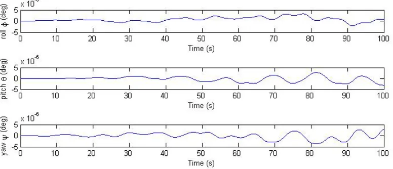
Figure 3.1: Error Euler angles of the QUEST algorithm with ideal noise-free IMU sensor measurements.
The results of simulations are shown in Figures (3.1-3.2). Figure (3.1) shows the error Euler angles versus time and indicates the satisfactory performance of the QUEST under ideal conditions. It can be seen that the algorithm is successful in obtaining optimized quaternions/rotation matrices from the very beginning. This is due to the fact that QUEST does not rely on attitude kinematics and the optimization process is performed in each time step.
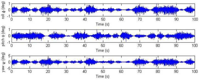
Figure 3.2: Error Euler angles of the QUEST algorithm with noisy measurements.
This is due to the fact that some parameters used in this algorithm (such as S andZ) are obtained from the vector multiplications of noisy vectors to each other. The same happens for the computation ofλmaxusing (3.75).
3.8.4
Filter QUEST
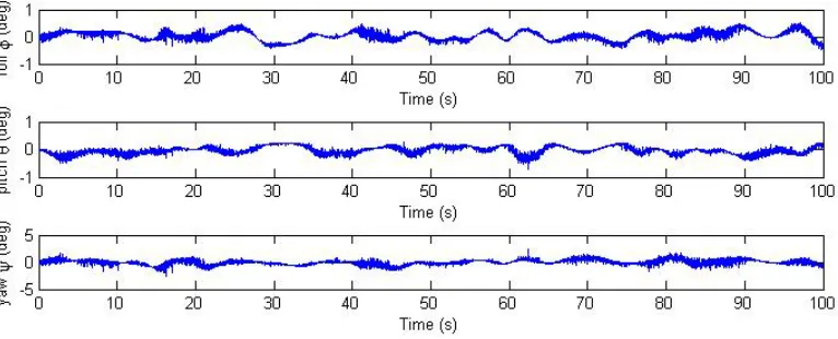
The recursive QUEST algorithms include the propagation of either B or K through the rotational dynamic equations. As discussed before, the two known recursive QUEST al-gorithms Filter QUEST and REQUEST are mathematically equivalent. However, the RE-QUEST is more computationally demanding since it requires the propagation of the matrix
K.
Figure 3.3: Error Euler angles of the Filter QUEST algorithm with noisy measurements.
3.9
Discussion
The static attitude reconstruction algorithms, specially the various QUEST-based methods discussed in this thesis, are aimed to find the optimal attitude given a set of vector observa-tions at a given time. Although the initial soluobserva-tions to Wahba problem did not consider the attitude kinematics, recursive forms of QUEST algorithm try to propagate the estimated attitude and covariance matrix over time, which results in better estimations.
In that sense, the recursive static algorithms are similar to Kalman filters and previ-ous studies have confirmed this similarity in the performance of the two distinct filters. While the propagation phase is a key part in the process of both filters, the most important difference resides in the way each method finds the optimal attitude.
The recursive methods, such as the Filter QUEST presented in the simulations, provide better estimations with regards to measurement noise. The propagation of profile matrix when observations are not simultaneously obtained, filters the available data and enhances the algorithm performance.
only degrading factor is the sensor measurement noise. For small-scale UAVs, however, the IMU set of magnetometers along with accelerometers might not result in good estimations by using this method due to the linear acceleration of the rigid body.
Dynamic Attitude Filtering and
Estimation
4.1
Introduction
The need for fast attitude estimation techniques that are able to adapt themselves to changes in system states and give more reliable estimations led to the development of dynamic filtering methods and observers. In these techniques, not only vectorial observations are used, but the system dynamics are exploited in the design strategy to capture and predict the behavior of the system.
As discussed in the previous chapter, the main disadvantage of the static attitude esti-mation methods is their inability to take the full system dynamics into account. In these methods, the attitude is estimated regardless of the nonlinear structure of system and only vectorial measurements were used. However, dynamic methods incorporate the system equations in estimation process and therefore, have the potential of providing better esti-mation results.
Probably the most popular dynamic attitude estimators are Kalman filters and its vari-ants such as the Extended Kalman Filter (EKF). These filters have the advantage of being specifically designed to work under noisy measurements conditions. The EKFs are
ear versions of the original Kalman filter and have been applied to many aerospace appli-cations during the last decades. A description of this type of filters is presented in section (4.2) along with their earliest applications in the forms of Multiplicative Extended Kalman Filters and Additive Extended Kalman Filters. More modern Kalman filtering techniques such as Unscented Kalman Filtering and Invariant Kalman Filters will also be covered in section (4.2). These will help the reader to become familiar with the use of these techniques for the attitude estimation problem.
The second main approach in dynamic attitude filtering is the complementary filtering. Along with Kalman filters, the complementary filters have been successful in providing re-liable attitude estimations under real-time conditions. As their name states, these filters use various sensor measurements to “complement” each other in obtaining a better estimation. Section (4.3) will be dedicated to a brief presentation of such filters.
The nonlinear observers are another major group of dynamic attitude estimators. In these estimation tools, ideal vectorial, position and velocity measurements are assumed.
conditions.
4.2
Extended Kalman Filters
The Kalman Filtering (KF) techniques in aerospace applications have been the subject of extensive research in the past few decades and the field has experienced huge progress from its original development in 1960’s [Grewal and Andrews, 2010]. From the original filter designed for linear systems to the forms compatible for nonlinear systems, the Kalman filters have been adapted to many estimation problems and have been applied to various actual missions.
While the basic Kalman filter was developed for linear systems, the technique can also be used for nonlinear systems provided that a linearization of the system in each step is performed about the best estimate state obtained in the previous step. The approach is called Extended Kalman Filtering (EKF) and has been the most widely used technique in real-time attitude estimation [Crassidis et al., 2007].
During the last decades, EKF has been successfully applied to many Aeronautics appli-cations [Toda et al., 1969b], [Farrell, 1967], [Garcfa-Velo and Walker, 1997]. The existing EKF approaches for the attitude determination differ in the parametrization of attitude.