F U L L P A P E R
Open Access
Some reasoning on the RELM-CSEP
likelihood-based tests
Anna Maria Lombardi
Abstract
The null hypothesis is the essence of any statistical test: this is basically a comparison of what we observe with what we would expect to see if the null hypothesis was true. In this work, I explore the suitability of the null hypothesis of likelihood-based tests (LBTs), which are often adopted by the laboratories of the Collaboratory for the Study of Earthquake Predictability (CSEP), to check earthquake forecast models. First, I discuss the LBT in the wider context of classical statistical hypothesis testing. Then, I present some cases in which the null hypothesis of LBT is not
appropriate for determining the merits of earthquake forecast models. I justify these results from a theoretical point of view, within the framework of point process theory. Finally, I propose a possible upgrade of LBT to enable the correct assessment of the forecasting capability of earthquake models. This study may provide new insights to the CSEP LBT.
Keywords: Statistical tests; Earthquake forecast; Point processes
Background
The increasing interest of the seismological commu-nity in earthquake forecasting has highlighted the need for a proper evaluation of forecast models. This has motivated the birth of the working group on Regional Earthquake Likelihood Models (RELM, Schorlemmer and Gerstenberger 2007) and of the Collaboratory for the Study of Earthquake Predictability (CSEP, Jordan 2006), both designed to evaluate the quality of forecast mod-els. The protocol adopted by RELM/CSEP is based on classical statistical hypothesis testing (Schorlemmer et al. 2007). This is then finalized to reject or accept the null hypothesis (hereinafter H0) on the basis of a numerical
summary of the data. RELM/CSEP working groups adopt two main types of testing methods: likelihood-based tests (LBTs) (Schorlemmer et al. 2007; Zechar et al. 2010) and alarm-based tests (ABTs) (Zechar and Jordan 2008). In this study, I focus on LBTs and specifically onN andL tests (Schorlemmer et al. 2007).
The RELM/CSEP working groups formalized the LBT to test hypotheses that ‘should follow directly the model, so that if the model is valid, the hypothesis should be consistent with data used in a test. Otherwise, the hypoth-esis, and the model on which it was constructed, can be
Correspondence: [email protected]
Istituto Nazionale di Geofisica e Vulcanologia, via di Vigna Murata, 605, Rome 00143, Italy
rejected’ (Schorlemmer et al. 2007). Actually, as I dis-cuss below, this intent was not attained (Lombardi and Marzocchi 2010a; Schorlemmer et al. 2007, 2010a; Werner et al. 2010).
The CSEP testing centers use theNandLtests to check the consistency of expected ( = {λ(i,j)}) and observed
( = {ω(i,j)}) values of variables X(i,j), representing the
number of earthquakes with magnitude above a thresh-oldMF, in nonoverlapping bins{(Ti,Rj);Ti ∈T,Rj∈ R} of a predetermined spatio-temporal spaceS = R× T (Jordan 2006; Zechar et al. 2010). A model is represented by forecasts, which are the only values provided by the modelers. The correct calculation of thepvalues of the LBT requires the probability distribution ofX(i,j)given by
the model and specifically the probabilities
pijn=P{X(i,j)=n} for n=0, 1, 2,. . . (1)
As this information is not available to modelers, the LBT assumes, as the null hypothesis H0, that the variables
X(i,j) are independent and follow a Poisson distribution
with meanλ(i,j). Therefore, the set of probabilitiespijnare substituted for the probabilities
qijn= [λ(i,j)]n
n! exp
−λ(i,j) for n=0, 1, 2,. . . (2)
and the p values of the LBT are computed accordingly (Schorlemmer et al. 2007).
Specifically, the N test measures the probability of observingNiO = jω(i,j) events, for each forecast time
period Ti. The pvalues of the N test are given by the probabilities (Zechar et al. 2010):
δ1=P(Xi≥NiO) δ2=P(Xi≤NiO), (3)
where Xi = jX(i,j). The RELM/CSEP protocol rejects
a model ifδ1 orδ2is too small, meaning that the model overpredicts or underpredicts the observed seismicity. Under H0, Xi is a Poisson variable with expectation NiF = jλ(i,j) (and PDF qin =[NiF]ne−N
F
i/n!), and the
percentiles δ1/δ2 are computed by this distribution (see
Schorlemmer et al. 2007).
The L-test measures the probability of the joint log-likelihoodL(i|)of observing, given the forecast.
The p value of the L test is estimated by comparing L(i|) with a predetermined number N of synthetic likelihood values L(Si|) = {L(Sl
i |),l = 1,. . .,N}, computed by Equation 4, of simulated catalogs ‘consis-tent with the forecast’ (Schorlemmer et al. 2007). This means that the forecast gridsSl
i are simulated accord-ing to the Poisson hypothesis supposed byH0, and thep
value of theLtest is given by the proportion of simulated log-likelihoods below the valueL(i|):
This shows that the LBT does not check the hypoth-esis that a forecast model has merit with the given data (marked hereinafter by Hyp1). Actually, the LBT tests whether{ω(i,j)}are independent random variables, from a
Poisson population with mean{λ(i,j)}(marked hereinafter
by Hyp2). When a model is not consistent with Hyp2, i.e., when the set of probabilities{pijn}is significantly different from{qijn}, the specific computation of thepvalues of the LBT is misleading, causing a potentially unjustified rejec-tion of the model itself (Lombardi and Marzocchi 2010a). The CSEP laboratories still systematically use the LBT, but a process of revision has begun. This study is intended to provide a contribution to this process.
Methods
A suitable revision of the LBT requires the full recognition and quantification of the causes and effects of the present inefficiencies. For this purpose, I apply theN andLtests to two classes of 1,000 simulated forecast grids, generated by different spatio-temporal magnitude models. In this
way, the data are perfectly known, and the rejection ofH0
cannot mean the failure of the model being tested. First, I generate two sets of synthetic catalogs. Each cata-log covers a time period of 1 month (January 1 to 31, 2012), the Italian collecting region, and a magnitude range of [2.5, 9.0], as chosen by CSEP (Schorlemmer et al. 2010b).
The first class of simulations is consistent with a version of the epidemic-type aftershocks sequence (ETAS) model (Ogata 1998), submitted to the CSEP-Italy testing region (Lombardi and Marzocchi 2010b). The rate of the model at timet, with location(x,y)and magnitudem, is given by: M0 andMmax are the minimum and maximum
magni-tudes,Ht = {(Ti,Xi,Yi,Mi);Ti < t} is the history (i.e., the information relative to past events) up to timet, and ri is the distance between location(x,y)and the epicen-ter of theith event(Xi,Yi)(see Lombardi and Marzocchi 2010b, for details). To compute the rateλ1(t,x,y,m/Ht), I include in the history the seismic bulletin of the Isti-tuto Nazionale di Geofisica e Vulcanologia (INGV) from April 16, 2005 to December 31, 2011. Moreover, I add a synthetic event (Tms,Xms,Yms,Mms) at time 00:00:00
on January 1, 2012 (Tms), with magnitude Mms = 6.0
and coordinates(Xms,Yms) = (13.384◦E, 42.346◦N). The
parameter values used in this study areμ= 0.7,K= 0.026, p= 1.15,c= 0.01,α= 1.4,d= 0.7,q= 1.5,γ = 0.3,b= 1.0, M0= 2.5, andMmax= 9.0.
To generate the ETAS forecasts for dayTi and catalog Ck, I mimic the CSEP real-time experiment: specifically, I include the triggering rate for events with historyHTi
ofCk and average the triggering rates of 1,000 simulated realizations of the process inside Ti (see Lombardi and Marzocchi 2010b, for details).
The second class of simulations follows a nonstationary poisson (NP) process. Specifically, the rateλ2(t,x,y,m)is
whereris the distance between(x,y)and(Xms,Yms). The
parameters used here areμ= 0.7,K= 0.1,p= 0.9,c= 0.02, α = 1.4, d = 0.7, q = 1.5, γ = 0.3, b = 1.0, M0 = 2.5,
Mmax= 9.0.
The simulations represent the average seismicity of the first month of a sequence (following a shock with magni-tude 6.0), as predicted by the ETAS and NP models. The basic difference between the models is that the rate of the ETAS model depends on the whole historyHt(i.e., infor-mation relative to past events), whereas the rate of the NP model depends on the coordinates of only one event (Tms,Xms,Yms,Mms). Thus, the rate of the NP model is
deterministic and decreasing in time fromTms, whereas
the rate of the ETAS model has a random nonmonotonic time evolution, depending on historyHt.
For each synthetic catalog, I compute the 1-day binned forecast grids(MF= 2.5) by integrating (in time, space, and magnitude) the rate of the model used to generate the catalog. The forecast gridscover a period of 1 month (starting from January 1, 2012) and the test spatial grid adopted for the CSEP Italian laboratory (Schorlemmer et al. 2010b). Finally, I apply the CSEP/RELMN and L tests (with significance level α = 0.05 andMF = 2.5) on all simulated catalogs, using the forecast grids previously computed.
In this paper, I propose an obvious upgrade of LBT, which does without the Poisson distribution. First, the discrete log-likelihood function L(i|) of variables Xi (Equation 4) is substituted for the continuous-time log-likelihood function (hereinafter, CLF). This is a proper measure of the agreement between model and data, taking into account the features of a model. For a spatio-temporal magnitude earthquake model, this is given by
CLF=
NRxTx[M0Mmax]
i=1
lnλ(ti,xi,yi,mi)
−
T
R Mmax
M0
λ(t,x,y,m)dtdxdydm (8)
where λ(t,x,y,m) is the rate of the model (Daley and Vere-Jones 2003) and NRxTx[M0Mmax] is the number
of events inside the spatio-temporal magnitude space RxTx[M0Mmax].
Second, the percentiles of the distributions of both the variablesXiand the CLF are derived directly by the model. This information allows the computation of more reli-able p values for the tests (Werner and Sornette 2008; Schorlemmer et al. 2010a).
In brief, the new testing procedure presented here con-sists of the following steps:
1. For each forecast periodTi, the number of events
(i) and the CLF (CLFM,i) of modelMbeing tested
are computed.
2. For eachTi,Ncatalogs given by modelMare simulated; the occurrences
SM,i=
Sl
M,i,l=1,. . .,N
and the likelihood
CLFSM,i=CLFSl
M,i,l=1,. . .,N
are computed for all catalogs.
3. The percentiles of the empirical distributions generated in the previous step, used to perform a test at the95%confidence level, are estimated.
Specifically, the 2.5th and 97.5th percentiles
P
M,i[2.5%]andPM,i[97.5%]
of valuesSi and the 5th percentilePCLFM,i[5%]of quantitiesCLFSM,iare identified.
4) The observed valuesiandCLFM,iare compared
with the percentiles computed in the previous step. In this way, modelMis rejected or retained forTi. Specifically, modelMis rejected ifi<PM,i[2.5%]
ori>PM,i[97.5%]or ifCLFM,i≤PCLFM,i[5%].
In this procedure, the percentiles of model Mare esti-mated by simulations because it is often not possible to derive them analytically. However, the use of simulations is not mandatory for modelers, of course.
Results
First, I apply the CSEP LBT to two classes of ETAS and NP simulations. Figure 1a shows the fraction of rejectionsFR (i.e., the proportion of catalogs for whichH0is rejected)
of theN andL tests as a function of time. As shown in Lombardi and Marzocchi (2010a),FRfor the ETAS simu-lations is well above 5%, which is the threshold justifiable by chance. On the other hand,FRfor the NP simulations is close to or below 5%, suggesting that Hyp2is consistent with the NP model.
To investigate whether previous results depend onMF or on the average seismic rate of the region, I apply the procedure described above to 1,000 new catalogs, repro-ducing the average seismicity of Japan (which has a seis-mic rate two orders of magnitude higher than that of Italy). These datasets are simulated by using anad hoc ETAS model of this region. In this experiment, I consider a fore-cast time spanTiof 3 months, an overall time period of 10 years, and MF = 4.0. This last value is the thresh-old magnitude adopted by the Japanese CSEP laboratory for short-term forecasting experiments (Nanjo et al. 2011; Tsuruoka et al. 2012). I find thatFRis equal to 40%to50% and 60%to75% for theN andLtests, respectively (see Figure 1b).
0 5 10 15 20 25 30 0
0.05
0.1 0.15 0.2 0.25 0.3
Time window (Ti, 1 day)
Fractions of rejections (F
R
)
ETAS, N-test
NP, N-test ETAS, L-test
NP, L-test
0 5 10 15 20 25 30 35 40
0 0.2 0.4 0.6 0.8 1
a)
b)
ETAS, N-test (CSEP)
ETAS, L-test (CSEP)
ETAS, N-test (new procedure)
ETAS, L-test (new procedure)
Time window (Ti, 3 months)
0.05
Figure 1Fraction of rejections.Application of CSEP/RELM LBT and the proposed testing procedure on simulated catalogs.(a)FRof daily CSEPN
andLtests, for ETAS and NP simulations of Italian seismicity andMF= 2.5.(b)Comparison ofFRvalues of testing procedure proposed here with
those obtained by CSEP/RELM LBT, for ETAS simulations of Japanese seismicity (MF= 4.0), with a forecast time span of 3 months.
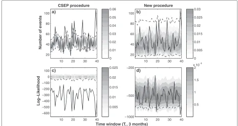
Figure 2 shows the PDF of occurrences and log-likelihoods computed by the CSEP LBT and the proposed proce-dure for the first ETAS simulated Japanese catalog. The observed occurrences (solid black line, Figures 2a,b) are well above or below the confidence bounds (dashed black lines, Figure 2a) of the Poisson PDF (Equation 1) supposed by Hyp2. This is because the distribution expected by the ETAS model (contour plot, Figure 2b), estimated by the empirical PDF ofSETAS,i, has a long/heavy tail, which is clearly not consistent with Hyp2. Similar results are found for the log-likelihood. The log-likelihoodsL(i|) com-puted by Equation 4 are well below the values ofL(Si|) expected by Hyp2(contour plot, Figure 2c). However, the log-likelihoods CLFETAS,i(Equation 8) are fully consistent with the log-likelihoods CLFSETAS,iexpected by the ETAS model (contour plot, Figure 2d).
Discussion
The rejection of the null hypothesis of a statistical test can be due to chance because it is really false or because it is probabilistically inadequate (Stark 1997; Luen and Stark 2008). The null hypothesis H0 of the RELM/CSEP LBT
supposes that X(i,j) are independent (in time and space)
and Poisson random variables, with meanλ(i,j), given by
the model. The CSEP protocol interprets the rejection of H0as the failure of the model being tested. However, this
procedure is misleading becauseH0is not consistent with
any model (Lombardi and Marzocchi 2010a).
The above findings may be explained with the help of stochastic point process theory (Daley and Vere-Jones 2003); this is the natural context in which stochastic earth-quake models may be discussed. A point process is fully represented by its ‘conditional intensity function’ (CIF) λ(t,x/Ht), i.e., the probability of observing an event in the instantt∈T and with additional variables (called marks)
x ∈ X, given the realization Ht of the process before t (Daley and Vere-Jones 2003). The CIF of the models described in the previous section are given by Equations 6 and 7; the marks are locations and magnitudes. In the case of an NP process, the CIF is a deterministic function of time and marks, but it is independent of the past his-tory (i.e., λ(t,x/Ht) = λ(t,x)). Therefore, the events in nonoverlapping subsets of T × X are independent and Poisson random variables (Daley and Vere-Jones 2003), as supposed by the RELM/CSEP LBT. In the most gen-eral case, the CIF is also a function of historyHt, and the variablesX(i,j) are not Poisson, unless the history is fully
Number of events
CSEP procedure
10 20 30 40
20 40 60 80 100
0 0.01 0.02 0.03 0.04 0.05 0.06
New procedure
10 20 30 40
20 40 60 80 100
0 0.005 0.01 0.015 0.02 0.025 0.03
Log−Likelihood
10 20 30 40
−600 −500 −400 −300 −200 −100 0 100
0.005 0.01 0.015 0.02 0.025
Time window (Ti, 3 months)
10 20 30 40
−1000 −500 −200
0.5 1 1.5 2 x 10⁻³
a) b)
c) d)
Figure 2Distribution of the number of events and of likelihoods for ETAS simulations.Contour plot of probability density as a function of time intervalTiof the number of events and likelihood for the first ETAS Japanese simulated catalog.(a)Contour plot of probabilitiesqinpredicted
by Poisson hypothesis Hyp2. Solid black line marks the observed number of events. Dashed black lines mark the 2.5th and 97.5th percentiles of distribution.(b)The same as(a)but for the distribution expected by ETAS model. Specifically, dotted lines mark the valuesP
ETAS,i[ 2.5%] and P
ETAS,i[ 97.5%].(c)Contour plot of PDF of log-likelihoodsL(i|)predicted by Poisson hypothesis Hyp2(Equation 4). Solid black line marks the observed log-likelihoods. Dashed black lines mark the 5.0th percentile expected by Poisson distribution.(d)The same as (c) but for the CLF (see Equation 8). Solid black line marks the observed values CLFETAS,i. Dotted black line marks the percentilePCLFETAS,i[ 5.0%].
The hypothesis Hyp2 has been questioned in sev-eral studies (Schorlemmer et al. 2010a; Werner et al. 2010) and, in the specific context of ETAS modeling, by Lombardi and Marzocchi (2010a). Here, I examine the causes and effects of the failure of the LBT. Specifically, I show that the failure of the LBT may be significant for high values ofMF and that it has heavy consequences for long forecast time windows. This is because the longer the forecast time windowTi, the greater the randomness of forecasts (due to the effect of the unknown history inside Ti) and the lower the reliability of Hyp2. This result con-tradicts the statement that the Poisson distribution is a good approximation of the forecast variability whenMFis large (Werner et al. 2010).
The process of revising the LBT has begun inside the scientific community. Some people have proposed replac-ing the Poisson distribution with a negative binomial distribution (Werner et al. 2010) to compute thepvalues of the tests. However, this solution does not significantly improve the LBT because the negative binomial distri-bution (as for the Poisson or any other distridistri-bution) is not consistent with all models. Inside the CSEP commu-nity, some suggest updating the forecasts more regularly,
leaving the LBT unchanged (personal communication). I do not think this is the best way to resolve the inefficien-cies of the LBT, as these do not derive from the regularity of the forecast calculations.
The procedure described above is an obvious upgrade of theNandLtests. It accounts for the actual variability of theX(i,j)given by the model being tested. Moreover, it uses
the CLF, which is a better tool for checking the agreement between models and data than the discrete log-likelihood (Equation 4) used by the CSEPLtest and based on Hyp2 (Schorlemmer et al. 2007).
components, especially in testing regions with a high seis-mic rate. In other words, the present study does not invalidate most of the results of the first RELM/CSEP forecast experiments, which focus on long-term time-invariant models. However, the inclusion of different fore-cast time-spans and time-dependent models in new CSEP experiments requires both an urgent revision of the test-ing procedure and an effort by modelers to provide full distributions of the variables being tested.
Conclusions
The main goal of this study was to interpret the fail-ures of the CSEP/RELM LBT and to propose a possible upgrade of theN andLtests. The main findings can be summarized as follows:
1. All LBTs are based on classical statistical hypothesis testing; therefore, they are intended to reject or not reject a null hypothesisH0. The null hypothesis of the LBT is that the variablesX(i,j)are independent and Poisson-distributed, with the rate given by forecasts. Therefore, the LBT is inadequate for checking the merits of a forecast model that is inconsistent withHyp2.
2. Specifically,Hyp2is not adequate for
history-dependent models, such as ETAS, because the unknown history inside the forecast period means thatX(i,j)do not follow a Poisson distribution. 3. In these cases, the LBT may fail for large values of
MF, especially for large forecast time windows, as the
effect of the unknown history is greater.
4. I propose a revised version of the LBT that (1) adopts the CLF and (2) requires the percentiles of the distributions ofXiandCLFM,i.
5. The points discussed in this study highlight the need to revise the testing procedure for present and future experiments, which include many time-dependent models. However, they have a relative effect on the first RELM/CSEP experiments, mainly focused on long-term time-independent models.
Competing interests
The author declares that she has no competing interests.
Acknowledgements
The author is grateful to W. Marzocchi (INGV) for stimulating discussions on the topics presented in this paper. The suggestions made by D.D. Jackson (UCLA) and two anonymous referees have significantly improved the quality of the paper. The Italy earthquake data were obtained from the seismic bulletin of the Istituto Nazionale di Geofisica e Vulcanologia (INGV, http://iside. rm.ingv.it). The Japan earthquake data were extracted by the Earthquake Catalog of the Japan Meteorological Agency (JMA, http://www.jma.go.jp/en/ quake). Information on CSEP is available at www.cseptesting.org.
Received: 15 October 2013 Accepted: 14 April 2014 Published: 1 May 2014
References
Daley DJ, Vere-Jones D (2003) An introduction to the theory of point processes. Second Ed, Vol. 1. Springer, New York, pp. 469
Jordan TH (2006) Earthquake predictability: Brick by brick. Seism Res, Lett 77(1): 3–6
Lombardi AM, Marzocchi W (2010a) Exploring the performances and usability of the CSEP suite of tests. Bull Seismol Soc Am 100: 2293–2300 Lombardi, AM, Marzocchi W (2010b) The ETAS model for daily forecasting of
Italian seismicity in the CSEP experiment. Ann Geophys 53: 155–164 Luen B, Stark PB (2008) Testing earthquake predictions. IMS Lecture Notes
Monograph Series. Probability and Statistics: Essays in Honor of David A. Freedman. Institute for Mathematical Statistics Press, Beachwood. 302-315 Meyer P (1971) Demonstration simplifiée d’un thèoréme de Knight In:
Sèminaire de, Probabilitès V. Univ. Strasbourg, Lecture Notes in Math. vol 191, pp. 191–195
Nanjo KZ, Tsuruoka H, Hirata N, Jordan TH (2011) Overview of the first earthquake forecast testing experiment in Japan. Earth Planets Space 63(3): 159–169
Ogata Y (1998) Space-time point-process models for earthquake occurrences. Ann Inst Statist Math 50(2): 379–402
Papangelou F (1972a) Summary of some results on point and line processes, in Lewis P.A.W. Stochastic Point Processes. Wiley, New York. pp. 522–532 Papangelou F (1972b) Integrability of expected increments of point processes
and a related random change of scale. Trans Amer Math Soc 165: 483–506 Schorlemmer D, Gerstenberger MC (2007) RELM Testing Center. Seismological
Res, Lett 78(1): 30–36
Schorlemmer D, Gerstenberger MC, Wiemer S, Jackson DD, Rhoades DA (2007) Earthquake likelihood model testing. Seism Res Lett 78(1): 17–29 Schorlemmer D, Zecher JD, Werner MJ, Field EH, Jackson DD, Jordan TH
(2010a) First results of the Regional Earthquake likelihood models experiment. Pure Appl Geophys 167: 859–876
Schorlemmer D, Christophersen A, Rovida A, Mele F, Stucchi M, Marzocchi W (2010b) Setting up an earthquake forecast experiment in Italy. Ann Geophys 53: 1–9
Stark PB (1997) Earthquake prediction: the null hypothesis. Geophys J Int 131: 495–499
Tsuruoka H, Hirata N, Schorlemmer D, Euchner F, Nanjo KZ, Jordan TH (2012) CSEP Testing Center and the first results of the earthquake forecast testing experiment in Japan. Earth Planets Space 64(8): 661–671
Werner MJ, Sornette D (2008) Magnitude uncertainties impact seismic rate estimates, forecasts, and predictability experiments. J Geophys Res 113: B08302. doi:10.1029/2007JB005427
Werner MJ, Zechar JD, Marzocchi W, Wiemer S (2010) Retrospective evaluation of the five-year and ten-year CSEP-Italy earthquake forecasts. Ann Geophys 53(3): 11–30. doi:10.4401/ag-4840
Zechar JD, Jordan TH (2008) Testing alarm-based earthquake predictions. Geophys J Int 172: 715-724. doi:10.1111/j.1365-246X.2007.03676.x Zechar JD, Gerstenberger MC, Rhoades DA (2010) Likelihood-based tests for
evaluating space-rate-magnitude earthquakes forecasts. Bull Seism, Soc Am 100(3): 1184–1195. doi:10.1785/0120090192
Zechar JD, Schorlemmer D, Werner MJ, Gerstenberger MC, Rhoades DA, Jordan TH (2013) Regional earthquake likelihood models I: first-order results. Bull Seism, Soc Am 103(2A): 787–798. doi.10.1785/0120120186
doi:10.1186/1880-5981-66-4