R E S E A R C H
Open Access
Modeling sets of unordered points using
highly eccentric ellipses
Demetrios Gerogiannis
*, Christophoros Nikou and Aristidis Likas
Abstract
An algorithm for modeling a set of unordered two-dimensional points by line segments is presented. The points are modeled by highly eccentric ellipses, and line segments are extracted by the major axes of these elongated ellipses. At first, a single ellipse is fitted to points which is then iteratively split to a large number of highly eccentric ellipses to cover the set of points. Then, a merge process follows in order to combine neighboring ellipses with almost collinear major axes to reduce the complexity of the model. Experimental results on various databases show that the proposed scheme is an efficient technique for modeling unordered sets of points and shapes by line segments. A computer vision application of the method is also presented regarding the detection of retinal fundus image features, such as end-points, junctions, and crossovers.
Keywords: Model fitting; Modeling by line segments; Line segment clustering; Ellipse eccentricity
1 Introduction
In many computer vision applications, at a mid-level pro-cess, it is common to fit line segments in order to model a set of unordered points so as to summarize higher level features. For example, the detection of vanishing points [1], the vectorization of raster images [2], and the detection of road structures and parts [3] are among appli-cations necessitating line segment description of image structures. In many of the aforementioned problems, the involved algorithms assume that they are provided with an ordered point set and standard polygonal approximation [4,5] is then applied. However, determining the order-ing of point sets is not a trivial task, and in the method described herein, we relax this assumption by making no prior hypothesis about the ordering of the points.
In the above context, the Hough transform (HT) is a widely used method for line fitting, and many variants have been proposed to improve its efficiency [6,7]. One of these variants is the randomized Hough transform (RHT) [8,9] which randomly selects a number of pixels from the input image and maps them into one point in the parameter space which was shown to be less complex, compared to the original algorithm, as far as time and
*Correspondence: [email protected]
Department of Computer Science and Engineering, University of Ioannina, Ioannina 45110, Greece
storage issues are concerned. In [10], the probabilistic HT was proposed whose basic idea is to apply a random sam-pling of edge points to reduce computational complexity and execution time. Further improvements were intro-duced in [11]. A similar concept was proposed in [12], where an orientation-based strategy was adopted to filter out inappropriate edge pixels, before performing the stan-dard HT line detection which improves the randomized detection process. Also, the idea of fuzziness is integrated in the main algorithm in [13] to model the uncertainty imposed to the contour due to noise. Thus, a point can contribute to more than one bin in the standard HT process. A general comparison between probabilistic and non-probabilistic HT variants can be found in [14].
The robust HT is introduced in [15] where both the length and the end-points of the lines may be computed. Moreover, the algorithm in [16] provides a method for adopting a shape-dependent voting scheme for the cal-culation of the histogram bins. Finally, a novel HT based on the eliminating particle swarm optimization (EPSO) is proposed in [17], to improve the execution time of the algorithm. The problem parameters are considered to be the particle positions and the EPSO algorithm searches the optimum solution by eliminating the ‘weakest’ parti-cles, to speed up the process.
Line segment fitting may also be used in a shape descrip-tion process. The commonly used algorithm of Moore
[18] was a first solution to shape following. However, this algorithm is appropriate only for traversing curves with-out intersections and produces models with high com-plexity, although improvements of the main algorithm have also been considered up to date [19]. Another com-mon model fitting method is the RANSAC algorithm [20], which despite the fact that it provides robust estimations, it is appropriate for fitting only one model at a time. Other approaches are the incremental line fitting [21] which is sensitive to noise and, most importantly, needs sequen-tial ordering of the points and probabilistic methods [22] based on the Expectation-Maximization algorithm, gen-erally necessitating the prior determination of the number of model components.
In this paper, we propose a method to model a set of unordered points by line segments. The result of the method is a sequence of straight line segments model-ing the points, which correspond to the major axes of highly eccentric ellipses fitted on them. We call the pro-cedure Direct Split-and-Merge algorithm or DSaM. The points may correspond to the locations of edge pixels. The basic idea relies on a split-and-merge process, where the algorithm is initialized by one ellipse, representing the mean and the covariance of the initial point set, which is then split, through an iterative scheme, until a number of small and elongated ellipses occurs. Then, a merge pro-cess takes place to combine the resulting ellipses in order to reduce the complexity of the representation. At the end, the algorithm provides a relatively small number of elon-gated ellipses fitted on the points. The proposed method is general and may also model a set of points containing inner structures, such as joints. Numerical experiments on common shape databases are presented to underpin the performance of the proposed method. Also, edgemaps of natural images were used in our experiments to ver-ify the efficiency of the method on real data. The number of ellipses depends on the structure of points, and it is determined by two parameters controlling both the split and the merge processes. The extension of the method to a three-dimensional (3D) case is trivial, as the elon-gated ellipses may be transformed to 3D ellipsoids. In the 3D case, our rationale is to model the points by highly eccentric ellipsoids, thus, instead of line segments, multi-ple 2D planes fit to points. In that case, data from range images could be modeled. A preliminary version of this method was introduced in [23]. Note that our method is not affected by degradations in the contour, and thus, it is more reliable compared to the distance transform [24] or the medial axis transformation [25], as it assumes more relaxed initial conditions (a set of unordered points) com-pared to conventional shape description methods, where point traversal should be knowna priori.
Moreover, we present some applications that could benefit by our DSaM method. To that end, an efficient
algorithm for retinal image analysis based on the pro-posed modeling framework is presented. More precisely, the purpose is to parse the image representing the retinal vessels and extract their characteristic points (end-points, junctions, and crossovers).
The remainder of the paper is organized as follows: In Section 2, the split-and-merge algorithm is presented. Experimental results using various databases (MPEG7 [26], GatorBait100 [27], ETHZ [28], Brown [29]) that con-tain either object silhouettes or collections of real images are shown in Section 3. In the same section, a compari-son of the proposed method with a variant of the Hough transform, namely, the progressive probabilistic Hough transform (PPHT) is demonstrated [30]. In Section 4, we present an applications of our method: an algorithm for retinal image analysis is presented along with its evalua-tion using the DRIVE database [31-33].
2 Direct split-and-merge method
Let X = {xi|i = 1,. . .,N} be a set of points and E = {j|j=1,. . .,K}be the set of line segments modeling the
points, whereiis the line describing theith segment.
We define the modeling errorinduced by the
repre-sentation of line segments:
whereK is the number of line segments the model uses
to model the points,xi ∈R2,i= 1,. . .,Nare the points,
d(xi,j)is the perpendicular distance of pointxito linej, δijis an indicator function whose value is one if pointxi
belongs to line segmentjand is zero otherwise.
In order to prevent overfitting, models having a large number of line segments should be penalized. Therefore, an optimal model would have both low value ofand low complexity.
The computation of the ellipses, modeling the line segments, is performed in two steps: an iterative split process, where points are modeled by a number of line seg-ments represented by the major axes of the corresponding ellipses and an iterative merge process, where small line segments are merged to reduce the model complexity. The split process tries to minimize the modeling error while the merge process decreases the model complexity, i.e., the number of line segments compared to the total number of points in the set.
What follows are the two steps presented in detail.
2.1 Split process
based on Gestalt theory [34], which models the linearity and the connectivity the human brain uses when modeling contours.
In order to split a setX, it should be either non-linear or disconnected, or both. Linearity describes how close the points are to a straight line, while disconnectivity mea-sures how concentrated these points are. In the ideal case, the covariance matrix of collinear 2D points should have a very large eigenvalue and a zero eigenvalue. The eigen-vector corresponding to the larger eigenvalue indicates the direction of the line segment. If the linearity property is relaxed, the less collinear the points become (i.e., they diverge from the linear assumption) the larger the value of the minimum eigenvalue is. Based on that observation, in our method, linearity is described by the minimum eigen-value of the covariance matrix of the points inX. Also, the disconnectivityWof two sets of pointsX,Yis the smallest distance between a point inXand a point inY:
W(X,Y)=min x∈X y∈Y
|x−y|. (2)
In the case of a single set, disconnectivity is the largest distance between two successive points in that set. It may be computed by projecting the points onto both axes defined by the eigenvectors of the covariance matrix of the set. Then, successive points are defined by scanning along the axes and their distances are computed. LetXibe
the projection of a setXonto the the eigenvectorei. The
disconnectivity ofXis defined as
W(X)= max
j=1,...,N−1
i=1,...,d
|xij−xij+1|, (3)
whereNis the number of points inX,dis the dimension ofX (hered = 2), and xij is thejth point of the sorted setXi. A large value of disconnectivity indicates a better
separation of the point sets. The projections onto all of the eigenvectors should be examined as we do not knowa prioriwhich direction to follow while splitting. Although intuitively one would suggest to split along the direction of the principal axis, we observed that in many cases that approach was not the best. Also, let us note that as the ordering of the points is not knowna priori, their pro-jection onto the eigenvectors of their covariance matrix, provides a natural way of ordering.
The disconectivity of a single set of points is also impor-tant to be estimated in the split step, as there may exist subsets that although they are linear, they are discon-nected, as it is demonstrated in Figure 1.
The split of an ellipse should be performed along the direction defined by an eigenvector of its covariance. In order to select the split direction, the axis corresponding to an eigenvector is considered as the discrimination bor-der between the split line clusters and points belonging
Figure 1An example of an instance of a split where a subset of the points is linear but disconnected.If the disconnectivity of the points was not considered a single line segment would summarize these points.
to the same subplane are grouped together. Then, the dis-connectivity of each line cluster is computed. Finally, the direction with the largest disconnectivity is selected for splitting (Figure 2).
Eventually, the adopted strategy that minimizesand prefers elongated ellipses can be expressed as follows: split every ellipse whose minimum eigenvalue is greater
than a threshold T1 (linearity) and the maximum gap,
within the current segment is greater than a thresh-old T2 (disconnectivity). The process is initialized with one ellipse, corresponding to the covariance of the ini-tial points set centered at the mean value of the point locations. ThresholdsT1andT2may be computed with a heuristic algorithm, as explained in Section 3.1.
At iterationt+1, a given ellipse, characterized by the eigenvaluesλt1 andλt2 of its covariance matrixt (with
λt1 ≥λt2), with centerμt, is split to two new ellipses with centers the two antipodal points on the major axis:
μt1+1=μt+√λtet,
μt2+1=μt−√λtet, (4)
whereet, λt are the eigenvector and the eigenvalue cor-responding to the split direction along which split is performed (Figure 2).
The points of the split ellipse are then reassigned to the two new ellipses according to the nearest neighbor rule. In this way, new ellipses occur, which are more elongated as they have greater eccentricity and their minor axes are closer to the contour (Figure 3). Moreover, this detailed representation of the point set provides accurate modeling of the joints, corners, and parts of the contour exhibiting high curvature.
A variant of the method would be to compute the covariance matrix of the points on the convex hull of the point set, which provide more robustness to outliers.
2.2 Merge process
(a)
(b)
Figure 2Split process.(a)At iterationt+1, the ellipse with centerμtis split into two new ellipsese1ande2, with centersμt1+1andμt2+1given by
(4).(b)The new centers are marked with a star (*). The reassignment of the points to the new centers is shown. Points of one category, assigned to e1, are marked with a square, while points assigned toe2are marked with a circle.
between the two line clusters is smaller than a threshold T2(disconnectivity).
Note that the threshold T1 could be set equal to the threshold used in the split process, where the value of parameterT1specifies whether an ellipse has low eccen-tricity and needs to be split. In the merge process, it indi-cates whether two candidates for merging ellipses would result in an ellipse with high eccentricity. One could use the same threshold in both processes, assuming the same significance. On the other hand, a relaxation of the merge threshold could lead to a rougher model of the points, smoothing out details like joints. In our experiments, the merge threshold was selected to be the same with the split threshold. The same applies for thresholdT2that indicates whether two segments are close enough to be considered as one line segment.
The overall description of the method is presented in Algorithm 1.
(c)
(d)
(a)
(b)
Figure 3Steps of the split-and-merge process.The process is initialized with the mean and the covariance of the full set of points. (a)Split into two ellipses.(b)Split into four ellipses.(c)End of split (35 ellipses).(d)The final merge result (23 ellipses). The figure is better seen in color.
Algorithm 1 Direct Split-and-Merge Algorithm
SPLIT PROCESS
input:The set of pointsX= {xi|i=1,. . .,N}. output:A set of ellipses{μj,j}.
Initialize the algorithm by estimating the mean and covariance of the point locations.
whilethere are ellipses to splitdo
Split every ellipse whose minor eigenvalue is greater thanT1and its disconnectivity is greater thanT2.
• Select the direction that provides the greatest disconnectivity.
• Set the centers of the new ellipses according to(4).
end while
MERGE PROCESS
input:The ellipses from the split processj= {μj,j}, j=1,. . .,M.
output:A reduced set of ellipses.
whilethere are ellipses to mergedo for allellipsesi,i=1,. . .,Mdo
if merging i with j provides an ellipse
whose minor eigenvalue is less than T1 and its disconnectivity is less thanT2then
Accept merging.
Setito the ellipse that result from merging end if
end for end while
3 Experimental results and discussion
Table 1 Short description of the databases used in our experiments
Database # Categories # Shapes/scenes Description
GatorBait100 [27] 8 38 Fish silhouettes
MPEG7 [26] 70 1,400 Object silhouettes
Brown [29] 13 137 Object silhouettes
ETHZ [28] 5 257 Real scene images
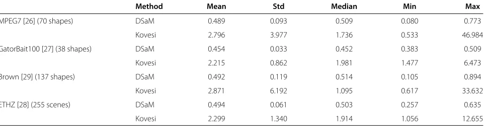
The shapes of this database are not closed and contain many junctions. The MPEG7 shape database [26] consists of 1400 silhouettes of various objects clustered in 70 cat-egories.The shape silhouette database used in [29], that contains 137 silhouettes of various objects, clustered in 13 categories, was also used in our experiments. Finally, to investigate the behavior of the proposed algorithm in real scene images, the images (257) from the ETHZ image set [28] were also used. Table 1 gives a brief description of each database. In all cases, the edges were extracted and the coordinates of the edge pixels were used to describe the contour. The Canny edge detector [35] was used in all cases.
3.1 Numerical evaluation
In this section, we present the resultsa of comparing the DSaM method with the widely used implementation of Kovesi [36]. Tables 2 and 3 summarize the numerical results, while Table 4 demonstrates the execution time for the experiments on MPEG7 [26], GatorBait100 [27], Brown [29], and ETHZ [28] datasets. Some representative images from those databases are given in Figure 4. As it can be observed, in some cases, there exist inner struc-tures and thus, the ordering of the points is not obvious. Note that to share common parameters, in the Kovesi [36] implementation, we used the disconnectivity thresh-old of our method. The execution time for computing that value is not included in the execution time of the Kovesi implementation. The model complexity is computed by the index:
MC= #ellipses
#points. (5)
Lower values of MC imply lower complexity and therefore a more compact representation.
The distortion is the measure of the quality of the fitting and is computed as the average distance between a point and its corresponding line segment, as computed by each method. Please note that the average length of the diag-onal of the bounding box of the various datasets is about 500 units (ranging from 300 units in Brown [29] to 700 units in ETHZ [28]).
In the proposed algorithm, there are two parameters
to be a priori specified, a threshold that determines
the elongation of an ellipse (T1) and a threshold
characterizing the disconnectivity of a set (T2).
Both parameters are used to decide whether to split (in the split process) or merge (in the merge process). A small value preserves the details, while a larger one provides more coarse results. For our experiments, we computed the values of the parameters as:
T1= 1
the smallest eigenvalue of the covariance matrix of points
{x|x∈Nα
Large values forαdecrease the model complexity pro-viding larger modeling error and details are not preserved.
In our experiments, we setα = 0.01×Nfor
comput-ing the values ofT1andT2. To make our implementation more efficient, instead of taking all points into consider-ation, we computed a random permutation of the indices of points and used only the first 10% of them. Thus, in
Table 2 Modeling error(1)
Method Mean Std Median Min Max
MPEG7 [26] (70 shapes) DSaM 0.489 0.093 0.509 0.080 0.773
Kovesi 2.796 3.977 1.736 0.533 46.984
GatorBait100 [27] (38 shapes) DSaM 0.454 0.033 0.452 0.383 0.509
Kovesi 2.215 0.862 1.981 1.477 6.473
Brown [29] (137 shapes) DSaM 0.492 0.119 0.514 0.105 0.894
Kovesi 2.871 6.192 1.095 0.617 33.632
ETHZ [28] (255 scenes) DSaM 0.494 0.061 0.503 0.257 0.635
Table 3 Model complexity MC (5)
Method Mean (%) Std (%) Median (%) Min (%) Max (%)
MPEG7 [26] (70 shapes) DSaM 3.954 0.013 3.788 0.269 11.429
Kovesi 3.624 0.017 3.406 0.269 12.442
GatorBait100 [27] (38 shapes) DSaM 3.280 0.004 3.172 2.732 4.541
Kovesi 2.524 0.005 2.378 1.961 3.904
Brown [29] (7 scenes) DSaM 5.792 0.016 6.186 0.921 10.145
Kovesi 6.586 0.022 6.911 0.335 10.821
ETHZ [28] (16 scenes) DSaM 5.342 0.014 5.195 2.436 8.427
Kovesi 5.402 0.018 5.205 1.601 11.040
high density datasets, like in the ETHZ database [28], the values of the thresholds could be estimated quickly.
In general, the DSaM method and the Kovesi imple-mentation produce models with similar complexity, a fact that is obvious, since they employ the same thresholds. However, the DSaM method provides much more accu-rate results w.r.t distortion (Tables 2 and 3). Concerning the execution time of the methods, one may observe that for simple datasets, like the object silhouettes [26,29], both methods are quite fast. However, for more complex datasets, like the ETHZ [28], DSaM is much faster (up to about eight times) than the Kovesi implementation, since these datasets, contain a lot of points and Kovesi implementation has to check them all, one by one.
As our method models the line segments with ellipses, we tried to fit line segments by exploiting various modifi-cations of a typical Gaussian Mixture Model (GMM) [37], for example, using an incremental GMM, or imposing constraints in the update step of the covariance matrices (decomposing the covariance matrices with SVD, replac-ing the correspondreplac-ing minimum eigenvalue with a very
small value, threshold T1, and then recomputing the
covariance matrix). All these variants failed to produce an efficient result. Moreover, the execution time was quite high (ten times compared to those of DSaM). Thus, we opted for excluding the results from this presentation.
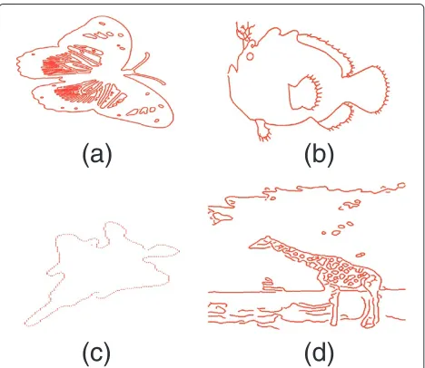
Finally, we conducted experiments to verify the robust-ness of the method against the presence of noise that degrades the contour of an object. To that end, we used three patterns (see Figure 5a,b,c) which were randomly repeated to create new images. A representative image is given in Figure 6. As a ground truth for the number of line segments, we used 4 for the square, 3 for triangle, and 10 for the star.
Table 4 Average execution time (in seconds)
Method MPEG7 GatorBait100 Brown ETHZ
DSaM 0.7 5.8 0.1 10.1
Kovesi 1.9 21.1 0.1 78.6
The set of unordered points was produced by simple edge detection. Then, zero mean Gaussian noise with varying standard deviation was added in order to get sev-eral configurations of signal-to-noise ratio (SNR). A repre-sentative result of a degraded contour is given in Figure 5d. Note that no ordering of points may be established in that case and thus polygon approximation may not be performed. To make the experiment independent from the noise configuration, each experiment was repeated 20 times. The algorithm assumes that a form of binary data (e.g., an edge map) is provided. Degradation by noise is performed after the edge extraction in order to exam-ine the behavior of the algorithm to the detection of lexam-ine segments. If the noise was added to the original image, the edges would be erroneous and we would not have a standard baseline for evaluating the algorithm.
In Figure 7, we present the results of the experiments. The error is expressed as the absolute difference between
(b)
(a)
(d)
(c)
(b)
(d)
(a)
(c)
Figure 5Images used to create the artificial dataset and a representative result of a degraded contour.(a, b, c)The primitive images used to create the artificial dataset for experiments with Gaussian additive noise.(d)Contour degraded by additive Gaussian noise of 18 dB.
the real number of segments and the one computed by our method. It can be observed that while the magnitude of the noise decreases, the error is also decreased. The dif-ference between true and estimated number of segments is generally small, 3 on average with low variance (±2 seg-ments), compared to the total number of line segments, 90 line segments on average, corresponding to 3% deviation
Figure 6A representative test image produced by randomly repeating the patterns of Figure 5a,b,c.
between true and estimated measurement. Thus, it could be claimed that the proposed method exhibits a consistent and efficient performance even if the contour is corrupted.
3.2 Comparison with the Hough transform
Since the proposed algorithm fits line segments to a set of points, we also tested it against the commonly used Hough Transform (HT). However, since the stan-dard HT is appropriate for fitting lines and not line seg-ments, we applied the Progressive Probabilistic Hough Transform (PPHT), as proposed in [30] and implemented in the OpenCV library [38]. The implementation of PPHT imposes three parameters: (1) a threshold, indicating the minimum number of points in a bin, in the line parame-ter space, in order to consider that the line is represented by a sufficient number of points, (2) the minimum length of a line segment, and (3) the maximum gap between line segments lying on the same axis. In our experi-ments, we fixed the last two parameters (after a trial and error procedure keeping those parameters that best fit the examined points) and varied the threshold. The obtained results for the PPHT exhibited significant irreg-ularities such as a large number of overlapping lines for the same segment. Also, the corners of the shapes were not correctly captured. Representative experiments on the MPEG7 dataset [26] are shown in Figure 8a,b,c while the solution of our DSaM algorithm is illustrated in Figure 8(d).
The PPHT is based on a histogram which correlates the accuracy of the result with the number of bins used. Also, a threshold must be established to eliminate lines with small participation in the final result. A small number of bins may lead to an underestimation of the number of segments, while a large number of bins increases the com-plexity of the model. As far as the threshold is concerned, its value may have similar effects in the final model. A large value may drop some segments, while a small value may be responsible for a large number of lines fitted, anal-ogous to a GMM with one component per point. A more important drawback of the PPHT is that many overlapping lines may model the same line segment. Figure 8 presents solutions of PPHT for a given set of points and various parameters values.
Figure 7Experimental results using the datasets of Figure 6.They demonstrate the performance of our method in presence of Gaussian additive noise in terms of model complexity error. The vertical axis represents the absolute error between the real number of segments and the one computed by our method.
(a)
(b)
(c)
(d)
Figure 8Representative experiments on the MPEG7 dataset and the solution of our DSaM.(a,b,c)Results of the PPHT algorithm to a set of points representing the shape of a bone (MPEG7 dataset) y varying the minimum number of points in a bin (namely, 5, 15, and 25). Only a small fraction of the lines is drawn for visualization purposes. Note the overlapping lines.(d)The result of our method. The figure is better seen in color.
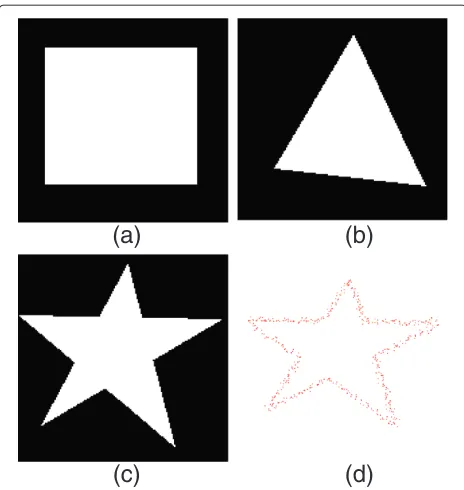
A methodology that extracts features from the retinal fundus image and characterizes them will be presented. The goal is to detect the intersection points between the vessels, as they could provide useful information to an automatic diagnosis system.
The detection and characterization of various topo-logical features of the retinal vessels are an important step in retinal image processing algorithms within an autonomous diagnosis system. A deviation from com-mon topological feature patterns may be an indicator of anomaly. A comprehensive study may be found in [41]. In a typical retinal vessel structure, more than 100junctions may be present [32], a fact that makes the manual char-acterization a tedious and time-consuming task. Typical retinal features are presented in Figure 9.
For our algorithm, three types of features are detected: end-points (points at the extremities of the vessels), interior-points (points along a vessel), junctions (a new vessel is a branch of a longer one -T-junctionsor a ves-sel is split into two or more new vesves-sels -bifurcation) and crossovers (one vessel passes over another). Please note that further processing is needed to distinguish between a crossoverand abifurcation.
Figure 9The different features that the proposed algorithm can detect.The yellow point is anend-point, the orange point is an interior-point, and the green point is acrossover. All the other points arejunctions(aT-junctionis shown in red, and abifurcationis shown in blue). The image is better viewed in color.
algorithm is to detectjunctions,crossovers, andend-points. The reader should refer to [42] or [43] for a detailed ves-sel extraction algorithm, which is a preprocessing step of the whole chain. At first, a Canny edge detector [35] is applied to extract the borders of the vessels and then a
(a)
(b)
(c)
(d)
Figure 10The original image, manual segmentation, data used in our retinal parsing algorithm, and confidence regions.(a)The original retinal image.(b)The manual segmentation of the vessels in (a).(c)Result of thinning the image in(b).(d)The confidence regions depicted as circles with a radius equal to 1% of the diagonal of the bounding box of the original set. The figure is better seen in color.
thinning algorithm [44] is used, to extract the center line of the vessels. In Figure 10a, the original image is shown. Figure 10b presents the manual segmentation, while the data used in our retinal parsing algorithm are shown in Figure 10c.
Once the center line of each vessel is extracted, the method presented in Section 2 is applied in order to extract the corresponding line segments and assign each point to its corresponding line segment. For each line segment, its extreme points are the points that have the largest distance from the corresponding extreme points of the same line cluster.
In Figure 11, the pointsx(summarizing the vessel struc-ture) are depicted with red and black color, while the cor-responding extreme pointsyare presented with green and blue dots. A rule is defined to characterize a point as end-pointorjunctionorcrossover. LetC(x)be the index of the line cluster point wherexbelongs to. In Figure 11, two line clusters are shown (C(x)=1 andC(x)=2). To define the neighborhood of extreme points, a neighborhood radius threshold is defined as
Tn=w∗ ¯d, (9)
whered¯ is the mean distance between all the nearest neighbors andwis a constant that is learned, as explained later in this section. Thus, for an extreme point y, the neighborhoodN(y) is the set of the points xsuch that
Figure 11An instance of the point characterization algorithm.
||x−y|| ≤Tn. Note thaty∈N(y). In order to
character-ize pointy, we defineCN(y)as the number of distinct line clusters that pointsx∈N(y)belong to.
In the example shown in Figure 11, the studied extreme pointyis the green one, while its neighborhoodN(y)is defined by a circle centered atywith radiusTn. Red and
black points lying within that circle are the neighbors of
y. Those points belong either to line cluster 1 or to line cluster 2 and thusCN(y)=2. If all neighbors ofybelong to the same line cluster with that of y, thenywould be anend-point(CN(y) = 1). In case whereCN(y) > 2,y
would be ajunctionor a crossover. The algorithm in its current form does not discriminate between them.
A special case occurs when CN(y) = 2, where the
studied point y is either an interior-point or a junction (T-junction). In that case, further elaboration is needed to characterize the extreme point by examining whether N(y)contains an extreme point or not. Thus, ifybelongs
also to the neighborhood of y, with y denoting the
neighbor of y, then y is an interior-point, otherwise it is a junction (T-junction). Please note that the neigh-boring relationship we are describing in that section is notreflective. For example in Figure 11, the green point, which is one of the extreme points of cluster 1, is neigh-bor to cluster 2 (as there are some points of cluster 2 within the yellow circle that defines the neighbor-hood of the green point). However, none of the extreme points of cluster 2 contain a point from cluster 1 in their neighborhood, and thus, cluster 1 is not neighboring to cluster 2.
In our example in Figure 11, this means that one of the two blue points would be inside the yellow circle. In case that N(y) contains no extreme point, as shown in Figure 11, then we compute the minimum distance (denoted bydin Figure 11) between the nearest neighbor (orange point in Figure 11) ofyamong the points of the other neighboring line cluster (black points in Figure 11) and the corresponding extreme points (blue points in Figure 11). Ifd ≤ ¯d, then yis a (junction) (T-junction), otherwise it is an interior-point.
A detailed description of the rules used to characterize an extreme pointyis presented in Algorithm 2.
Note that since the ground truth refers to the original vessels and not to their center lines, which is the input of our method, we determined a valueTconf that defines a confidence region around a ground truth point. A com-puted point is considered to match a ground truth point if it lies in its confidence region. In our experiments,Tconf is defined as a percentage (1%) of the length of the diag-onal of the bounding box of pointsx. Figure 10d shows the confidence regions depicted as circles with a radius equal to Tconf. To establish a robust value for constant
w ((9)), the precision and recall rates were computed
for values of w between 1.8 and 4.0 with a step of 0.8.
Then, the F measure (harmonic mean) was calculated
as
F=2 PR
R+P, (10)
Algorithm 2 Rules for vessel features characterization input: An extreme point y computed by the DSaM algorithm and the corresponding set of vessel skeleton pointsx∈N(y).
output:The label ofy.
ifCN(y)=1then yis anend-point.
else ifCN(y)=2then
yis either ajunctionor aninterior-point.
• Q= {x∈N(y)|C(x)=C(y)}
ifthe line cluster of points ofQis equal to C(y)then
yis aninterior-point
else
yis ajunction (T-junction).
end if • else
yis ajunction (T-junction).
• end if
else ifCN(y) >2then
yis ajunction(bifurcation) or acrossover.
end if
wherePis the precision andRis the recall:
P= TP
TP+FP, (11)
R= TP
TP+FN, (12)
where TP is the number of true positives, that is, the number of relevant items retrieved, FP is the number of false positives, that is, the number of irrelevant items retrieved and FN is the number of false negatives, that is, the number of relevant items not retrieved.
Figure 12 shows the plot ofF measure for various val-ues of parameterwin Equation (9). In our experiments,
the F measure takes its maximum value for w = 2.9.
The corresponding point is depicted with a black square in Figure 12. In that case, the corresponding precision is equal to 91.59% while the recall is 98.58%. The value of
¯
dcomputed from our experimental data is approximately equal to √2, which leads to Tn = 4.10, Equation (9),
corresponding to a neighborhood radius equal to 4 pixels. The mean execution time was 109 s for the extraction of the line segments and 12 s for the extraction and charac-terization of features using Matlab on a typical Dual Core
2×2.50 GHz machine with 2.0 GB RAM.
5 Conclusion
The problem of fitting several lines in order to describe a set of 2D unordered points is crucial in several com-puter vision applications. To that end, a split-and-merge algorithm was presented in this paper that iteratively fits a number of elongated ellipses to 2D points (DSaM). The points are represented by the major axes of the ellipses, while the minor axes account for possible perturbations from the linear modeling. Furthermore, a merge pro-cess combines neighboring ellipses with collinear major axes in order to reduce their number and consequently the complexity of the solution. An important aspect of the algorithm is that it does not require an ordering of the points and accurately handles contours or edge chains that contain joints and multiple structures.
The proposed method depends on two thresholds that control the flexibility of the model. Robust estimation of those parameters, in an adaptive scheme is an issue that need further elaboration and is a subject of ongo-ing research along with the application to other problems of methods [28,45,46] that could directly benefit from an effective solution to this problem.
Endnote
aMatlab code available at http://www.cs.uoi.gr/~
dgerogia
Competing interests
The authors declare that they have no competing interests.
Received: 13 November 2013 Accepted: 15 January 2014 Published: 28 January 2014
References
1. V Cantoni, L Lombardi, M Porta, N Sicard, Vanishing point detection: representation analysis and new approaches, in11th International Conference on Image Analysis and Processing (ICIAP)(Palermo, 26–28 September 2001), pp. 90–94
2. D Dori, L Wenyin, Sparse pixel vectorization: an algorithm and its performance evaluation. IEEE. Trans. Pattern. Anal. Mach. Intell.
21(3), 202–215 (1999)
3. S Se, M Brady, Road feature detection and estimation. Mach. Vis. Appl.
14(3), 157–165 (2003)
4. U Ramer, An iterative procedure for the polygonal approximation of plane curves. Comput. Graph. Image Process.1, 244–256 (1972) 5. A Kolesnikov, ISE-bounded polygonal approximation of digital curves.
Pattern Recognit. Lett.33, 1329–1337 (2012)
6. J Illingworth, J Kittler, A survey of the Hough transform. Comput. Vis. Graph. Image Process.44(1), 87–116 (1988)
7. VF Leavers, Which Hough transform? CVGIP: Image Underst.
58(2), 250–264 (1993)
8. L Xu, E Oja, P Kultanen, A new curve detection method: Randomized Hough Transform (RHT). Pattern Recognit. Lett.11, 331–338 (1990) 9. RA McLaughlin, Randomized Hough transform: improved ellipse
detection with comparison. Pattern Recognit. Lett.19, 299–305 (1998) 10. N Kiryati, Y Eldar, AM Bruckstein, A probabilistic Hough transform. Pattern
Recognit.24(4), 303–316 (1991)
11. J Matas, C Galambos, J Kittler, Progressive probabilistic Hough transform, inBritish Machine Vision Conference (BMVC), vol. I (London, September 1998), pp. 256–265
12. K Chung, Z Lin, S Huang, Y Huang, HM Liao, New orientation-based elimination approach for accurate line-detection. Pattern Recognit. Lett.
13. V Chatzis, I Pitas, Fuzzy cell Hough transform for curve detection. Pattern Recognit.30(12), 2031–2042 (1997)
14. H Kälviäinen, P Hirvonen, L Xu, E Oja, Probabilistic and non-probabilistic Hough transforms: overview and comparisons. Image Vis. Comput.
13(4), 239–252 (1995)
15. M Atiquzzaman, MW Akhtar, A robust Hough transform technique for complete line segment description. Real Time Imaging1, 419–426 (1995) 16. C Chau, W Siu, Adaptive dual-point Hough transform for object
recognition. Comput. Vis. Image Underst.96(1), 1–16 (2004) 17. HD Cheng, Y Guo, Y Zhang, A novel Hough transform based on
eliminating particle swarm optimization and its applications. Pattern Recognit.42(9), 1959–1969 (2009)
18. GA Moore, Automatic scanning and computer process for the quantitative analysis of micrographs and equivalent subjects, inPictorial Pattern Recognition(Thompson Book Co, Washington, DC, 1968), pp. 275–362 19. C Li, Z Wang, L Li, An improved Hough transform algorithm on straight line
detection based on Freeman chain code, in2nd International Congress on Image and Signal Processing (ICISP)(Tianjin, 17–19 October 2009), pp. 1–4 20. MA Fischler, RC Bolles, Random sample consensus: a paradigm for model
fitting with applications to image analysis and automated cartography. Commun. ACM24(6), 381–395 (1981)
21. P Bhowmick, B Bhattacharya, Fast polygonal approximation of digital curves using relaxed straightness properties. IEEE Trans. Pattern Anal. Mach. Intell.29(9), 1590–1602 (2007)
22. J Leite, E Hancock, Iterative curve organisation with the EM algorithm. Pattern Recognit. Lett.18(2), 143–155 (1997)
23. D Gerogiannis, C Nikou, A Lykas, A split-and-merge framework for 2D shape summarization, in7th International Symposium on Image and Signal Processing and Analysis (ISPA)(Dubrovnik, 4–6 September 2011), pp. 206–211
24. R Azriel, J Pfaltz, Sequential operations in digital picture processing. J. Assoc. Comput. Mach.13(4), 471–494 (1966)
25. DT Lee, Medial axis transformation of a planar shape. Pattern Anal. Mach. Intell., IEEE Trans.4(4), 363–369 (1982). doi:10.1109/TPAMI.1982.4767267 26. Temple University, College of Science and Technology. MPEG-7 dataset.
http://www.dabi.temple.edu/~shape/MPEG7/dataset.html. Accessed 27 January 2014.
27. University of Florida, GatorBait 100. http://www.cise.ufl.edu/~anand/ GatorBait_100.tgz. Accessed 27 January 2014
28. V Ferrari, T Tuytelaars, LV Gool, Object detection by contour segment networks, inEuropean Conference on Computer Vision(Springer-Verlag, Berlin Heidelberg, 2006), pp. 14–28
29. TB Sebastian, PN Klein, BB Kimia, Recognition of shapes by editing their shock graphs. IEEE Trans. Pattern Anal. Mach. Intell.26(5), 550–571 (2004) 30. J Matas, C Galambos, J Kittler, Robust detection of lines using the
progressive probabilistic Hough transform. Comput. Vis. Image Underst.
78, 119–137 (2001)
31. JJ Staal, MD Abramoff, M Niemeijer, MA Viergever, B van Ginneken, Ridge based vessel segmentation in color images of the retina. IEEE Trans. Med. Imaging23(4), 501–509 (2004)
32. G Azzopardi, N Petkov, Detection of retinal vascular bifurcations by trainable V4-like filters, in14th International Conference on Computer Analysis of Images and Patterns (CAIP)(Seville, 29–31 August 2011), pp. 451–459
33. G Azzopardi, N Petkov, Retinal fundus images - Ground truth of vascular bifurcations and crossovers. http://www.cs.rug.nl/~imaging/databases/ retina_database/retinalfeatures_database.html.
Accessed 27 January 2014.
34. D Marr,Vision(Freeman Publishers, New York, 1982)
35. J Canny, A computational approach to edge detection. IEEE Trans. Pattern Anal. Mach. Intell.8, 679–698 (1986)
36. PD Kovesi, MATLAB and Octave Functions for Computer Vision and Image Processing, Last Visited on September 3rd 2013. Centre for Exploration Targeting, School of Earth and Environment, The University of Western Australia. Available from: http://www.csse.uwa.edu.au/~pk/research/ matlabfns/. Accessed 27 January 2014
37. CM Bishop,Pattern Recognition and Machine Learning (Springer, Dordrecht, 2006)
38. G Bradski, A Kaehler,Learning OpenCV: Computer Vision with the OpenCV (O’Reilly Media, Sebastoupol, 2008)
39. Y-Y Chiang, CA Knoblock, A method for automatically extracting road layers from raster maps, in10th International Conference on Document Analysis and Recognition (ICDAR)(Barcelona, 26–29 July 2009), pp. 838–842 40. D Gerogiannis, C Nikou, A Lykas, Fast and efficient vanishing point
detection in indoor images, in21st International Conference on Pattern Recognition (ICPR)(Tsukuba, 11–15 November 2012)
41. N Patton, TM Aslam, MacT Gillivray, IJ Dearye, B Dhillonb, RH Eikelboomf, K Yogesana, IJ Constablea, Retinal image analysis: concepts, applications and potential. Prog. Retin. Eye Res.25, 99–127 (2006)
42. C Lemaitre, M Perdoch, A Rahmoune, J Matas, J Miteran, Detection and matching of curvilinear structures. Pattern Recognit.44, 1514–1527 (2011) 43. M Sofka, CV Stewart, Retinal vessel extraction using multiscale matched
filters, confidence and edge measures. IEEE Trans. Med. Imaging
25(12), 1531–1546 (2006)
44. RC Gonzalez, RE Woods,Digital Image Processing, 3rd edn. (Prentice Hall, Upper Sddle River, 2008)
45. V Ferrari, F Jurie, C Schmid, From images to shape models for object detection. Int. J. Comput. Vis.87(3), 284–303 (2010)
46. J-P Tardif, Non-iterative approach for fast and accurate vanishing point detection, in12th International Conference on Computer Vision (ICCV) (Kyoto, 27 September–04 October 2009), pp. 1250–1257
doi:10.1186/1687-6180-2014-11
Cite this article as:Gerogianniset al.:Modeling sets of unordered points
using highly eccentric ellipses. EURASIP Journal on Advances in Signal
Processing20142014:11.
Submit your manuscript to a
journal and benefi t from:
7 Convenient online submission 7 Rigorous peer review
7 Immediate publication on acceptance 7 Open access: articles freely available online 7 High visibility within the fi eld
7 Retaining the copyright to your article


![The effect of web based depression interventions on self reported help seeking: randomised controlled trial [ISRCTN77824516]](data:image/gif;base64,R0lGODlhAQABAIAAAP///wAAACH5BAEAAAAALAAAAAABAAEAAAICRAEAOw==)