Mechanical Engineering Department, Bu-Ali Sina University, Hamedan, Iran
Abstract. Dynamic behavior of materials is investigated using different devices. Each of the devices has some restrictions. For instance, the stress-strain curve of the materials can be captured at high strain rates only with Hopkinson bar. However, by using a new approach some of the other techniques could be used to obtain the constants of material models such as Johnson-Cook model too. In this work, the restrictions of some devices such as drop hammer, Taylor test, Flying wedge, Shot impact test, dynamic tensile extrusion and Hopkinson bars which are used to characterize the material properties at high strain rates are described. The level of strain and strain rate and their restrictions are very important in examining the efficiency of each of the devices. For instance, necking or bulging in tensile and compressive Hopkinson bars, fragmentation in dynamic tensile extrusion and petaling in Taylor test are restricting issues in the level of strain rate attainable in the devices.
1. Introduction
A wide variety of dynamic materials testing machines with different capabilities have been developed across the world. Generally, dynamic testing of materials can be categorized as intermediate (10−1–102s−1) or high strain rate (102–104s−1). Strain rates higher than 104s−1 usually correspond to the phenomena involved in shock wave propagation. The Intermediate strain rate testing techniques utilise air, hydraulic or mechanical testing machines. The piston type machine designed by Maiden and Green [1] is a typical example of the first category. The second category comprises hydraulic testing machines such as the advanced hydraulic torsion testing machine developed by Lindholm [2], which was capable of creating a continuous range of strain rates from quasi-static to 500 s−1. In mechanical testing machines, the required energy is usually stored in a large moving mass such as a fly wheel. One of the earliest types of dynamic mechanical testing machines was built by Nadia and Manjoine [3]. In this machine, the flywheel rotates at a constant angular velocity. At the time of impact, a hammer which is supported by a spring is suddenly released and is engaged with the base of the specimen. Another testing machine which is capable of producing a uniform strain rate is the cam plastometer [4]. In Much of the experimental work on the high strain rate response of materials involves the use of the most universally accepted high rate testing apparatus, the split Hopkinson bar (SHB), also known as the Kolsky bar, with different loading modes, including tension [5], compression [6], and shear [7]. Strain rates up to 104s−1 can be attained by the SHB. An alternative dynamic tensile testing facility, known as the Flying Wedge, which is capable of generating strain rates from 102s−1up to in excess of 104s−1, has been developed and used at Leeds University for several decades [8].
2. The high strain rate features
Some of the objectives in dynamic tests which look to be of more importance are described in following sections.
2.1. Strain and strain rate distribution
Strain rate is often obtained approximately from V/H where V is the deformation velocity and H is the gauge length of the specimen. But this relation is too rough and in some cases not true at all. In Hopkinson bar strain rate is calculated from:
dεs(t)
dt =−
2C0 L εR(t).
Where,εR(t)is the stress wave reflected into the input bar.
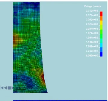
The strain rate is obviously constant before necking in tension and bulging in compression. The distribution of strain rate obtained in Taylor test is illustrated in Fig.1. As it is seen strain rate is not uniform within the specimens. Therefore, talking of strain rate in a test is basically nonsense. As a matter of fact, strain rate is a local quantity that is nonuniformly distributed within the specimen and varies from point to point in time and space.
2.2. Stress-strain curve and material models
Material models are widely used in finite element codes for analysis of material deformations particularly at high strain rates and elevated temperatures. Each material model has some constants which are determined using stress-strain curves obtained by experiment. The problems such as necking and bulging limit the conventional test techniques to measure the stress-strain curves only up to small strains. This is while, in some deformation processes, the strain can be greater than 1. Over the past recent years, a combined experimental, numerical and optimization approach has been used for determination of the constants. The method is explained in Sect. 5. The flow stress is defined in terms of strain, strain rate and temperature through some material models a number of which are given below:
Johnson-Cook [9]:
σ =A+Bεn 1+C Ln(ε˙/ε0)˙ 1−T∗ m
Figure 1.Strain rate distribution in a Taylor test specimen.
Zerilli-Armstrong [10]:
σ =C1+C2exp (−C3T +C4TLn (˙ε)) +C5εn for fcc
σ =C1 +C2 √
εexp(−C3T +C4TLn (˙ε)
for bcc.
2.3. Damage models
Determination of the constants of damage models are also one of the main objectives in dynamic tests. Two of the most important models are:
Analytical Gurson, Tvergaard and Needleman model [11]:
φ=
σe
σ0(¯ε) 2
+2q1f cosh
−3 2
σm
σ
−1+q12f2=0.
Empirical Johnson-Cook damage model [12]: εf =
D1+D2E X P
D3
P/σy
(1+D4Lnε)˙
1+D5T∗
.
2.4. Fracture mechanism
Fracture mechanism of a material may change from a pure ductile under quasi-static conditions to pure brittle under dynamic loading. Typical fracture surfaces are shown in Fig.2. Therefore, fracture mechanism is one of the major concerns in high strain rate deformations.
2.5. Fragmentation
Fragmentation occurs in high rate impacts or deformations. Typical example is shown in Fig. 3. Fragmentation is a restricting event in high rate testing techniques. For instance, fragmentation in Taylor test limits the plasticity in the specimens. However, some testing techniques such dynamic tensile extrusion have been innovated to study the fragmentation behavior of materials at high strain rates.
Figure 2. A pure brittle and (b) a pure ductile fracture mechanism.
Figure 3.Fragmentation in a ballistic test [13].
Figure 4.A general view of the “Flying wedge”.
3. Experimental methods
The experimental methods as explained in Sect. 1 are various. However, some of the most important ones which have wider application and the newest ones and their features are explained in the following sections.
3.1. Flying wedge
A general view of this apparatus is shown in Fig. 4. The slider mechanism, shown in Fig. 5, consists of two sliders with chamfered faces, the angle of which match up precisely with the wedge angle, together with two rails which allow the sliders to move freely, and two shock absorbers. Specimens are fitted between two specimen holders that are located within the sliders. When the gas gun is fired, the wedge plate connected to the piston rod accelerates quickly and hits the sliders. As a consequence of the impact, the sliders move rapidly away from each other resulting in tensile loading of the specimen.
Figure 5.The slider mechanism and the specimen.
V=328 m/s V=487.2 m/s
Figure 6.Typical specimens after Taylor test.
3.2. Taylor test
Taylor test was initially proposed by Taylor [16] in 1948 aiming at the study the ballistic behavior of metals. It relates the dynamic properties of the materials to the quasi-static one. His analysis is based on stress wave propagation in the specimens due to the impact of the projectile against a rigid target. The analysis takes account of the mushroomed profile of the specimen after impact. Today, Taylor test is still widely used for the study of dynamic behavior of materials at high strain rates along with numerical simulation. It is also used in inverse engineering such as the method explained in Sect. 5 for determining the parameters of material models.
Typical specimens deformed in Tayor test are illustrated in Fig. 6. As the figure indicates, when the impact velocity increases, the specimens deformation changes from a quite mushroomed shape to a shape which consists of two quite distinct regions; an undeformed region and a petal zone. The petaling limits the strain and strain rates achievable in Taylor test on one hand but provides means to study the petaling phenomenon itself on the other hand.
3.3. Inverse Taylor test
In this technique, the target (specimen) and the projectile (striker) swap their positions as usually considered in the conventional Taylor test (see Fig. 7) [17]. This type of test configuration eliminates the difficulties which are normally associated within situheating up the specimen. However, strain rates in inverse Taylor test is considerably lower than that in Taylor test. The reason is that the projectile (Target) in inverse Taylor test is much heavier than that (specimen) in Taylor test and consequently, the impact velocity in Taylor test would be much higher.
Figure 7.The schematic view of the inverse Taylor test [17].
Figure 8.A tensile Hopkinson bar apparatus.
3.4. Hopkinson bar
Hopkinson bar consists mainly of three bars, striker, incident and transmission bars [5–7]. The general view of a Hopkinson bar is shown in Fig.8. The striker bar is driven by a gas gun and hits the incident bar. A stress wave is produced and travels down the incident bar toward the specimen. In Hopkinson test method, the signals including the incident wave,εI, reflected wave,εR, and transmitted
wave,εT are used to calculate the torque, strain, stress and
strain rate in the specimen as follows [5]. dεs(t)
dt =−
2C0 L εR(t)
εs(t)=−
2C0 L
t
0
εR(t).dt
σs(t)=E
Ab
As
εT(t).
Where, E,C0,Ab,As,L are the Young modulus, elastic wave speed, cross sectional area of the bars, initial cross sectional area and initial length of the specimen, respectively.
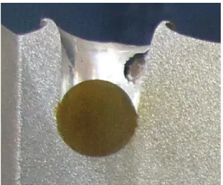
3.5. Shot impact test
Figure 9.The section of the shot inside the crater [19].
Figure 10.The process of DTE [18].
the experimental stress strain curve to large strains which may not be true in reality.
The constants of the material model correspond to the case when the experimental and numerical geometries of the craters created by the shot impact on the specimen coincide. The coincidence can be achieved by an optimization process such as genetic algorithm. The shot impact test is confined to plasticity without damage. Therefore, it appears to remain dominated solely by plasticity even at the upper velocities.
3.6. Dynamic tensile extrusion
In dynamic tensile extrusion (DTE) proposed by Gray et al. [19] several years ago, a spherical projectile (specimen) is shot through an open conical die in which the exit diameter of the die is smaller than the sphere diameter, the projectile undergoes severe dynamic tension at high strain rates. A simulation of the process is shown in Fig. 10. The order of strain rate is 104/s which is less than those seen in shot-impact tests and even Taylor tests. Dynamic Tensile Extrusion (DTE) is mostly used for studying the fracture mechanism particularly for determining the ductile to fracture transition in materials especially in polymers, although it has been used by Bonora et al and a few others for adjusting some material models. DTE is quite an interesting method by which the effect of material’s microstructures on macro-structural response of materials such as fragmentation and damage can be studied.
3.7. Drop hammer
In this device a dropping weight as the hammer hits the specimen which is mounted on an anvil. This device is
Figure 11.The dimensions used for optimization of final profile.
mainly used to study the behavior of energy absorbers. However, it can be used for compressive test and even tensile test too. This test provides medium strain rates. It lacks most of the capabilities of the dynamic test devices and even universal testing rigs.
3.8. Universal devices
Universal machines are the commercial testing apparatuses which are mainly used mechanical characterization of materials under quasi-static and low rate loadings. The universal machines such as Instron, Zwick, MTS, Avery, etc are among the most frequently used machines in the world. These machines lacks most of the capabilities of high rate testing machine such as the capabilities to study fragmentation, fracture mechanism transformation, erosion and other features which occur only in high rate deformations. However, these machines enjoy capabilities such as providing stress-strain curve, cyclic test for studying the damage evolution or isotropic/kinematic hardening of material.
4. Inverse engineering and material
model
As explained above, dynamic stress-strain curves are rigorously converted into material models which are highly important elements in the simulation of material deformation. In a new strategy called as “inverse engineering”, the dynamic stress-strain curve is eliminated from the test procedure and the constants of the material model are determined in a way that the difference between the experimental and the numerical load-displacement curves or the shape of dynamically deformed specimens is minimized [20,21]. This is performed by a combined experimental, numerical and optimization technique. The difference is taken as the objective function of an optimization problem. which can be defined by a function such as a polynomial as follows:
O B J(x)∼=a0 +
n
i=1 aixi +
n
i,j=1
bi jxixj. (1)
In which xi (i=1 to n) is the model parameters
vector, the coefficients ai andbi j are identified from the
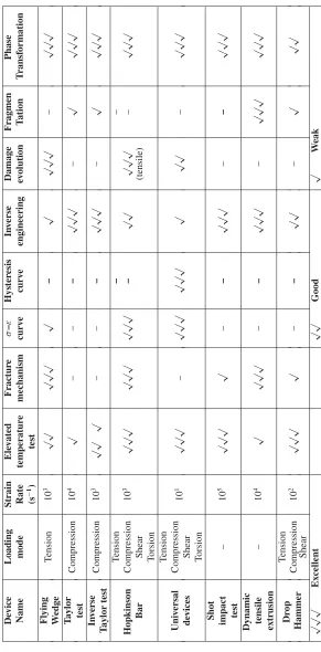
Ta b le 1 . The ev aluation o f v arious parameters in dynamic testing d ev ices. De vice Loading Strain Ele v ated Fractur e σ – ε Hyster esis In v erse Damage Fragmen Phase Name mode Rate temperatur e mechanism cur v e cur v e engineering ev olution Ta ti o n T ransf ormation (s − 1) test Flying T ension 10 3 √√ √√√ √ – √ √√√ – √√√ We d g e T aylor Compression 10 4 √ – – – √√√ – √ √√√ test In v erse Compression 10 3 √√ √ – – – √√√ – √ √√√ T aylor test T ension – – Hopkinson Compression 10 3 √√√ √√√ √√√ – √√ √√√ – √√√ Bar Shear (tensile) T o rsion T ension Uni v ersal Compression 10 1 √√√ – √√√ √√√ √ √√ – √√√ de vices
Shear Torsion
In this figure,a1=Lf anda3 =Dfare the final length
and the final end diameter of the specimen, respectively. The variablea2 =Xf is the length of the specimen which
has not experienced any deformation during the impact. The objective function is defined as follows:
O B J = O B JI2
+O B JI I2
+O B JI I I2 (2)
O B JI =a1experimental−a1numerical
=Lfexperimental−Lf numer i cal (3)
O B JI I =a2experimental−a2numerical
=Xfexperimental−Xfnumerical (4)
O B JI I I =a3experimental−a3numerical
=Dfexperimental−Df numer i cal. (5)
The terms aiExperimental−aiNumerical (i=1,2,3) represent the differences between the numerical and experimental profiles of the specimen for the three designated dimensions shown in Fig.11.
5. Summary and Conclusions
The results of this study are summarized in Table1. Each method clearly covers a range of strain rate. Therefore, the methods may not be comparable with each other in some respects. However, it is extremely important to know the capabilities of each method and its restrictions. As Table1indicates, some test methods are excellent for the study of some quantities or phenomenon but are useless for others. For instance, although a few techniques can be used for investigating fragmentation but dynamic tensile extrusion method is the best choice for this purpose. This is while this method is inefficient in other respects. It can be observed that the best equipments for capturing stress-strain curve are Hopkinson bars. Nevertheless, all methods can be employed for determining the constants of material models by inverse engineering as explained in Sect. 4. Flying wedge and tensile Hopkinson bar are the most appropriate devices for the study of fracture mechanism at high strain rates. These devices are also the best choices for the study of damage evolution which is a subject of damage mechanics. The specimens should be deformed to a controlled level and voids initiation, growth and
methods.
References
[1] C.J. Maiden and S.J.Green, J. app. mech.,33, 4961– 4970 (1966).
[2] U.S. Lindholm Techniques of metal research, 199– 253 (1967).
[3] Nadia A. and Manjoine M.J., Trans. ASME,63, A77 (1941).
[4] E. Orowan, B.I.S.R.A. Report MW/F/22/50, (1950). [5] J. Harding, E.D. Wood and J.D.Campbell, J. of Mech.
Eng. Sci.,2, 89, 88–96 (1960).
[6] T.V.T Yeung-Wye-Kong, Ph.D. Thesis, Mech. Eng. Dep. Leeds Univ. (1972).
[7] J. Duffy, J.D. Campbell and R.H. Hawley, Trans. ASME: J. Appli. Mech.,38, 83–91 (1971).
[8] B.N. Cole and J.L. Sturges, Int. J. Imp. Eng.,28, 891– 908 (2003).
[9] G.R. Johnson and W.H. Cook, 7th int. symp. Ballistics, 541–547 (1983).
[10] F.J. Zerilli, R.W. Armstrong, J. Appl. Phys.611816– 1825 (1987).
[11] A.L. Gurson, Ph.D. Thesis, Brown University, USA (1975).
[12] G.R. Johnson, W.H. Cook, Engng Fract Mech, 21, 31–48 (1985).
[13] http://www.cusatis.us/?p=820
[14] G.H. Majzoobi, A Hosseini, A Shahvarpour, Part I: experiments: Steel research int.79, 685–692 (2008). [15] G.H. Majzoobi, A Hosseini, A Shahvarpour, Part II: Simulation, Steel research int.79, 712–718 (2008). [16] G.I. Taylor, Proc. R. Soc. Lond. A, 194, 289-299
(1948).
[17] G.H. Majzoobi, P. Kazemi, M.K. Pipelzadeh, J. Exp. tech., In press, (2014).
[18] G.H. Majzoobi, A. Hosseinkhani, M.K. Pipelzadeh, S.j. Hardy, J Strain Analysis,49(5) 342–351 (2014). [19] Gray, G.T., Cerreta, E., Yablinsky, C.A., Addessio,
L.B., Henrie, B.L., Sencer, B.H., Burkett, M., Maudlin, P.J., Maloy, S.A., Trujillo, C.P., Lopez, M.F., AIP Conf. Proc.,845, 725–728 (2005). [20] G.H. Majzoobi, F. Freshteh Saniee, S. Khosroshahi,
H. Beikmohammadloo, Part I: Experiments and simulations, Computational Material science, 49, 192–200 (2010).